Samenvatting. In X-ray imaging, it is common practice to normalize the acquired projection data with averaged flat fields taken prior to the scan. Unfortunately ...
Dynamic intensity normalization using eigen flat fields in X-ray imaging Vincent Van Nieuwenhove1 , Jan De Beenhouwer1 , Francesco De Carlo2 , Lucia Mancini3 , Federica Marone4 , Jan Sijbers1 12 oktober 2015 Samenvatting In X-ray imaging, it is common practice to normalize the acquired projection data with averaged flat fields taken prior to the scan. Unfortunately, due to source instabilities, vibrating beamline components such as the monochromator, time varying detector properties, or other confounding factors, flat fields are often far from stationary, resulting in significant systematic errors in intensity normalization. In this work, a simple and efficient method is proposed to account for dynamically varying flat fields. Through principal component analysis of a set of flat fields, eigen flat fields are computed. A linear combination of the most important eigen flat fields is then used to individually normalize each X-ray projection. Experiments show that the proposed dynamic flat field correction leads to a substantial reduction of systematic errors in projection intensity normalization compared to conventional flat field correction.
1
Introduction
In X-ray imaging, the acquired projection images generally suffer from fixed-pattern noise, which is one of the limiting factors of image quality. It may stem from beam inhomogeneity, gain variations of the detector response due to inhomogeneities in the photon conversion yield, losses in charge transport, charge trapping, or variations in the performance of the readout [1]. Also, the scintillator screen may accumulate dust and/or scratches on its surface and in the bulk, resulting in systematic patterns in every acquired X-ray projection image. In X-ray Computed Tomography (CT), fixed-pattern noise is known to significantly degrade the achievable spatial resolution and generally leads to ring or band artifacts in the reconstructed images [2, 3, 4]. This, in turn, hampers quantitative analysis and complicates post processing such as noise reduction or segmentation [5]. If the pattern noise is truly stationary (i.e., exactly the same in each acquired projection image), substantial reduction of fixed pattern noise is easy. The conventional method to reduce fixed-pattern noise is known as flat field correction (FFC) [6]. Projection images without sample are acquired with and without the X-ray beam turned on, which are referred to as flat fields and dark fields. The flat fields include the non-uniform sensitivity of the charge-coupled device (CCD) pixels, the non-uniform response of the scintillator screen, as well as the inhomogeneities of the incident X-ray beam. Based on the acquired flat and dark fields, the measured projection images with sample are then normalized. While conventional FFC correction is an elegant and easy procedure that largely reduces fixedpattern noise, it heavily relies on the stationarity of the beam, scintillator response and CCD 1
sensitivity. In practice, however, this assumption is only approximately met. Indeed, detector elements are characterized by intensity dependent, nonlinear response functions and the incident beam often has time dependent non-uniformities [7], which renders conventional FFC inadequate. In synchrotron X-ray tomography, there is an even broader array of time dependent fluctuations. A range of components of the synchrotron cause beam variability: instability of the bending magnets of the synchrotron, temperature variations due to the water cooling in mirrors and the monochromator, or vibrations of the scintillator and other beamline components [8]. The latter is responsible for the biggest variations in the flat fields. The variation of the total incident X-ray intensity over time is another cause of flat field variation. Synchrotrons working in ’top-up’ mode inject, at regular times, new electrons into the storage ring, resulting in a typical saw-tooth function of the X-ray flux over time [9]. As a result, after conventional FFC, often significant intensity variation remains in the sinogram, leading to ring artifacts in the reconstructed image as concentric arcs or half-circles with varying intensity. Little work has been presented so far to deal with temporal fluctuations in the flat fields. In [8], an adaptive time-dependent intensity normalization was proposed in which the flat field is modelled by the product of a multiplicative function defined by dust or dirt on the surfaces of the scintillator and CCD camera, and a function describing a time dependent intensity profile of the X-ray beam incident on the sample. In [10], a FFC method together with an automated scanning mechanism was proposed in which the flat field images and projection data are acquired every view alternately. When acquiring the flat field image, the imaging sample is moved away from the field-of-view by a computer controlled linear positioning stage. While such a procedure allows view-by-view normalization, the mechanical set-up significantly lengthens the acquisition time. Moreover, it requires perfect repositioning of the sample, which is non-trivial. In our work, we propose a general, fast and simple method to account for time dependent variations in the flat fields. It estimates the flat field at the acquisition time of the projection in order to normalize the projection individually. Firstly, the technique performs a Principal Component Analysis (PCA) of flat fields acquired prior, during and/or posterior to the X-ray tomographic experiment [11]. Afterwards, the weights of the most important PCA components are estimated for each projection, minimizing a total variation criterion [12]. The estimated flat field is then used to normalize the corresponding projection.
2
Method
In this section, we will revisit the conventional FFC method (subsection 2.1), which is the standard normalization technique in X-ray imaging. Next, in subsection 2.2, the proposed dynamic FFC algorithm is described, which deals with non-stationary flat fields.
2.1
Conventional flat field correction
The attenuation of a monochromatic X-ray beam is described by the Beer-Lambert law, stating that: � Z � p = I0 · exp − µ(l) dl (1) with p the outgoing intensity, I0 the incoming intensity, µ the R attenuation coefficient of the object and l the coordinate along the X-ray path. The integral µ(l) dl is the total attenuation of the beam along a given ray. 2
Prior to the reconstruction of a cross section or volume, the projection data are normalized with respect to I0 : � � Z p µ(l) dl = − ln (2) I0 In practice, an estimate of p as well as I0 can be obtained from projections with and without object, respectively. This normalization procedure is known as flat field correction (FFC). Conventional FFC relies on a dark field, a flat field, and the projection image to be normalized: Dark field : A dark field d, often referred to as the offset field, is an image which is captured by the detector without X-ray illumination. The signal detected in the absence of X-rays from the X-ray source includes both the true dark current (which is proportional to the exposure time), and the digitization offset, which is independent of exposure time. Usually, the exposure time for the acquisition of dark field images is equal to that of the projection images. Flat field : A flat field f , often referred to as a white field or gain field, is acquired with X-ray illumination, but without the presence of the sample. It is used to measure and correct for inhomogeneities in the X-ray beam intensity profile and detector response. Projection image : projection images {pj } are acquired with X-ray illumination and the sample is positioned in the field of view of the detector. These images are acquired while the sample rotates, usually in regular angular intervals. Based on these images, an intensity normalized image nj is computed as follows: nj =
pj − d f −d
(3)
Since f as well as d contain noise, the variance of the normalized image nj is larger than the variance of pj , due to noise propagation. To limit this effect, d and f are replaced in practice by the average of a large number of dark and flat fields, d¯ and f¯, respectively [1].
2.2
Dynamic flat field correction
Conventional FFC as described in subsection 2.1 is only valid if the flat fields are stationary (i.e., do not change over time). If this is not the case, FFC based on a simple averaged flat field will introduce a bias in the normalized image. We propose an advanced FFC method that accounts for higher order dynamics in the flat fields. Thereby, each projection is normalized individually with its corresponding flat field: nj =
pj − d¯ fj − d¯
(4)
with fj the flat field at the acquisition moment of projection pj . Since fj is unknown, it has to be estimated. The main idea is to first capture the dynamics in the flat fields from a set of flat fields (acquired prior, during or after the experiment) and next exploit the dynamics to individually normalize each projection image. This will be explained in a more formal way in the following subsections.
3
2.2.1
Eigen flat fields
Let f ≡ {fn } ∈ RN a column vector representing a flat field (i.e., a vector composed of concatenated columns of a 2D projection with N pixels). If M flat field images are acquired, these images can be stored in a flat field matrix F ≡ {fm } = (f1 , ..., fM ) ∈ RN ×M . Let f¯ represent the mean flat field. Then, each flat field fm can be represented in a low dimensional (K � N ) space using PCA. That is, it can be well approximated by a linear combination of K eigen flat fields {uk }, the principal components, as follows: K X ¯ fm ≈ f + wmk uk (5) k=1
Computation of eigen flat fields Turk and Pentland proposed an efficient procedure to compute the eigen images [13]: Given a set of M flat fields F = (f1 , ..., fM ), a centered flat field matrix A ∈ RN ×M is computed by subtracting the mean flat field f¯ from each individual flat field: A = (f1 − f¯, ..., fM − f¯)
(6)
The goal is then to find the eigen vectors and eigen values of the covariance matrix C = AAT . Since C ∈ RN ×N is a huge matrix, calculating its eigenvectors is computationally expensive. Fortunately, as shown by Turk and Pentland, this problem can be efficiently dealt with by computing the eigenvectors {vi } and eigenvalues {λi } of the M × M matrix AT A. Then, {Avi } = {uk } and {λi } are the eigenvectors, referred to as eigen flat fields (EFFs), and eigenvalues of C, respectively. Selection of the eigen flat fields Once the EFFs are computed, the most important EFFs (i.e., the EFFs describing most of the variation in the flat fields) have to be selected. Many criteria exist to select an optimal number of Principal Components (EFFs), such as the Kaisers criterion, the cumulative percentage of total variation, or the scree test [14, 11]. In our work, we opted for a statistically justified approach based on parallel analysis [15]. Parallel analysis selects only those components of which the eigenvalues are significantly larger than the corresponding eigen values of a dataset with the same variation but with independent variables. To this end, a large number (S) of matrices with the same dimensions as A are sampled from a multivariate normal distribution with a diagonal covariance matrix of which the elements are identical to those of the covariance matrix C. Then, PCA is conducted on these matrices and the eigenvalues {λi,s }Ss=1 are collected. If λi of C is larger than the 95th percentile of the set {λi,s }Ss=1 of the covariance matrix of the sampled matrices, the ith EFF is retained. Filtering of the eigen flat fields In the previous step, the EFFs were selected that describe most of the variation in the flat fields. Compared to the remaining EFFs, the signal-to-noise ratio (SNR) of the selected EFFs is much higher, but obviously not noiseless. To limit noise propagation in the dynamic FFC method proposed in section 2.2.2, the selected EFFs are filtered using a block matching filter [16]. 2.2.2
Dynamic flat field estimation
Once the EFFs are computed from the set of flat fields acquired prior, during and/or posterior to the actual measurements, each measured projection is normalized with its corresponding flat field
4
fbj (see Eq. (4)). This flat field is generated by linearly combining K principal EFFs: fbj = f¯ +
K X
w ˆjk uk
(7)
k=1
where {w ˆjk } denote the estimates of the weights corresponding to the EFFs. The goal is then to find these weights such that the estimated flat field fbj approaches the true flat field fj . We assume that, if this is the case, the variation in the normalized projection nj is minimal. Total variation minimization Finding the optimal weights of the flat fields, {w ˆjk }, is accomplished by searching for the linear combination that minimizes the total variation (TV) in each normalized projection nj . However, simply minimizing TV(nj ) would lead to ever increasing weights {w ˆjk }. Indeed, the TV of an image i is a homogeneous function of degree one for a ∈ R+ , i.e. TV(a i) = a TV(i). Consequently, minimizing TV promotes images with a low mean. To prevent the algorithm favoring normalized projections with high valued flat fields, the TV is multiplied with c({wjk }), the mean of the applied flat field. This results in the following optimization problem: (8)
! K X � nj ({wjk }) = pj − d¯ / f¯ + wjk uk − d¯
(9)
{wjk }
with
N X
|∇nj ({wjk })|n
{w ˆjk } = arg min c({wjk }) ·
n=1
k=1
and
N K X 1 X ¯ fn + wjk uk,n − d¯n c({wjk }) = N n=1
! (10)
k=1
PN The factor n=1 |∇nj ({wjk })|n of the objective function, which is minimized in Eq. (8), denotes the TV of the normalized projection: T V (nj ). The objective function is minimized using a quasi-Newton method[17]. This nonlinear optimization algorithm is an alternative to Newton’s method in which the Hessian is approximated, reducing the computational cost of the algorithm. Two stopping criteria are used: a tolerance level of 10−6 and a maximum number of iterations (400). The weights {wjk } are estimated from down sampled projections and EFFs. This has two advantages: for one, the effect of noise on the TV is significantly reduced, resulting in a more robust estimation. Secondly, it substantially increases the speed of the algorithm. Intensity rescaling The TV criterion is sensitive to structural changes but insensitive to image offsets. Hence, we propose a rescaling of the projections after normalization. This procedure is different for truncated and non-truncated projections. Truncated projections are rescaled such that they have the same mean as the conventional flat field corrected projections. For non-truncated parallel beam projections the first Helgason-Ludwig consistency condition is used [18], stating that the sum of all the attenuation coefficients should be the same in every projection. Each dynamic flat field corrected non-truncated projection is rescaled such that they have the same mean as that of the full conventional flat field corrected dataset. An overview of the dynamic FFC algorithm is shown in Fig. 1. 5
parallel analysis
Figuur 1: Overview of the dynamic FFC algorithm.
3
Experiments
To validate the dynamic FFC methodology, simulations (section 3.1) as well as real experiments (section 3.2) were performed. All reconstructions were computed using the ASTRA tomography toolbox [19, 20].
3.1
Simulation study
A 3D spatial resolution software phantom (see Fig. 4) was generated on a 768 × 768 × 200 voxel grid. The Astra toolbox was used to simulate 500 log corrected projections with parallel beam geometry and an angular range 180 degrees [19]. A set of real flat fields of a foam imaging experiment (see section 3.2.2), 250 prior and 250 post flat fields, were applied on the simulated projections as described by the Beer-Lambert law (Eq. (1)): pj,sim = fj · e−nj
(11)
with nj the j’th simulated projection, fj the j’th flat field of the foam dataset and pj,sim the j’th projection with simulated dynamic flat fields. This procedure essentially simulates realistic dynamic flat fields. The remaining 50 prior and 50 post flat fields of the foam datasets were used to correct the projections with the conventional FFC as well as to compute the EFFs in the dynamic FFC. All flat fields were filtered with Non-Local Means to reduce noise [21]. In a first experiment, the number of flat fields and the number of EFFs were varied between 5 to 49 and 1 to 5, respectively. In a second experiment, the number of projections was varied from 5 to 500 in steps of 10, all with an angular range of 180 degrees. Two EFFs, calculated from a set of 100 flat fields, were used for dynamic FFC. All reconstructions were made using SIRT with 300 iterations. Both the normalized projections and corresponding SIRT reconstructions were assessed visually and quantitatively. To quantify the results, the Mean Squared Error (MSE) of the normalized projections as well as the MSE of the reconstructions was computed. The MSE in the projection domain was calculated on all projection data and the reconstruction MSE was calculated in a 100 × 100 region of interest (ROI) (see Fig. 4).
6
(a)
(b)
Figuur 2: (a) Mean posterior flat field of the aluminum peroxide dataset. (b) The first projection of the aluminum peroxide dataset.
3.2
Experimental data
The dynamic FFC algorithm was tested on two X-ray tomography datasets, each from a different synchrotron facility, and compared to conventional FFC. 3.2.1
Aluminum peroxide
At the Advanced Photon Source (APS) of the Argonne National Laboratory, a tomography dataset of an aluminum peroxide structure was acquired. The dataset consisted of 1 dark field, 100 posterior flat fields and 1500 equiangular projections, with an angular range of 180 degrees. Each of the projections (2048 × 2048 pixels) was acquired with an exposure time of 300 ms. The mean of the posterior flat fields and a projection are shown in Fig. 2. The dataset was processed using conventional as well as dynamic FFC. The dynamic flat field weights {wjk } were estimated on 20 times down sampled projections and afterwards applied to the full scale projections. Due to the limited amount of truncation the dynamic FFC projections were rescaled using the first HelgasonLudwig consistency condition [18]. Filtered Back Projection (FBP) reconstructions were made using the ASTRA toolbox [6, 19, 20]. 3.2.2
Foam
A ROI tomographic dataset of a foam structure was acquired at the Tomcat beamline of the Swiss Light Source (SLS) of the Paul Scherrer Institute (PSI). The dataset consisted of 20 dark fields, 300 prior flat fields, 251 projections and 300 posterior flat fields. Each projection (256×1248 pixels) was acquired with an exposure time of 30 ms. The mean flat field and a projection are shown in Fig. 3. The dataset was processed using conventional FFC and dynamic FFC, with one up to five EFFs. The dynamic flat field weights {wjk } were estimated on 20 times down sampled projections and afterwards applied to the full scale projections. Cross sections of the dataset were reconstructed with 200 iterations of SIRT and with FBP.
7
Figuur 3: (a) Mean of the prior and posterior flat fields of the foam dataset. (b) The first projection of the foam dataset.
4 4.1 4.1.1
Results and discussion Simulation study Number of EFFs and flat fields
Figure 4 shows the results of conventional and dynamic FFC (500 projections, 100 flat fields and 2 EFFs) on both the projections and the reconstructions. The projections with conventional FFC clearly suffer from vertical stripes in the sinogram due to flat field variations. These artifacts are almost completely removed with dynamic FFC. The effect of flat field variation manifests itself as broad ring artifacts in the reconstruction, which are also clearly visible in the error image. Both the reconstruction and error image based on dynamic FFC show a substantial reduction of these artifacts. In Fig. 5, the MSE of the projections and reconstructions is shown for conventional and dynamic FFC in function of the number of flat fields and EFFs. It can be observed that the MSE of the projections decreases slowly in function of the number of flat fields. Increasing the number of flat fields obviously improves the SNR of the EFFs and, as a result, improves the quality of the dynamic FFC projections. The MSE of the projections also decreases when more EFFs are used, although higher order (4th and 5th) EFFs only have a limited effect on the projection quality. This behavior was expected, as increasing the number of EFFs improves the description of the estimated flat fields as long as they contain sufficient structural information. The MSE of the reconstructions shows a more complex behavior. In general, the reconstruction quality improves with an increasing number of flat fields, which is to be expected, mainly because the increase of SNR of the EFFs. For a rather small number of flat fields (< 30), dynamic FFC with only 1 EFF performs best in terms of MSE. If more flat fields are available, the SNR of the second EFF is sufficiently high, hence improving the normalization when taking the second EFF into account. The use of more flat fields results in less noisy high order EFFs that enable a better description of the actual structural variation. In practice, as many flat fields as possible should be acquired to obtain a high SNR of at least the low order EFFs. Parallel analysis (cfr. section 2.2) indeed suggests a similar number of EFFs: one EFF if less than 33 flat fields are acquired and two
8
Conventional FFC
Dynamic FFC
Error image
Reconstruction
Sinogram
Ideal
Figuur 4: Sinograms, reconstructions and error images of slice 129 for conventional FFC and dynamic FFC are shown. For the dynamic FFC of the 500 projections, 2 EFFs, based on 100 flat fields, were calculated. The red square in the phantom images indicates the ROI in which the MSE was calculated.
Figuur 5: MSE of the projections (left) and the reconstructions (right) for both conventional FFC and dynamic FFC with 1 to 5 EFFs in function of the number of flat fields.
9
Figuur 6: MSE of the projections (left) and the reconstructions (right) for both conventional FFC and dynamic FFC (100 flat fields, 2 EFFs) in function of the number of projections. EFFs if 33 to 49 flat fields are used. It is clear that dynamic FFC outperforms conventional FFC in terms of projection MSE for all numbers of flat fields. Furthermore, dynamic FFC generally leads to improved reconstruction (quantified by the reconstruction MSE). 4.1.2
Number of projections
Figure 6 shows the MSE in the projection (left) and reconstruction domain (right) for conventional and dynamic FFC in function of the number of projections. Clearly, the MSE of the projections decreases substantially if dynamic FFC is used instead of conventional FFC. After conventional FFC, one can observe large variation in MSE as a function of the number of projections. In contrast, after dynamic FFC, there is almost no variation of the MSE as a function of the projections, which indicates that even severely distorted projections are properly corrected. The MSE of the reconstructions is in all cases slightly lower for the dynamic FFC than for the conventional FFC. This difference decreases with increasing number of projections. This can be explained by the back projection during reconstruction in which the remaining errors after FFC are averaged out.
4.2 4.2.1
Experimental data Aluminum peroxide
The aluminum peroxide EFF’s structure consists mainly of horizontal stripes (see Fig. 7), with decreasing intensity with increasing order of EFF. The EFFs clearly reveal structural variation in the flat fields as otherwise, only random noise would have been present in the EFFs, being the only source of variation. A projection of the aluminum dataset, corrected with conventional and dynamic FFC with 1 to 5 EFFs is shown in Fig. 8(a) and Fig. 8(b-f), respectively. The majority of the projections that are processed with conventional FFC are degraded by horizontal stripes over the whole width of the projection. In contrast, dynamic FFC is able to remove most of the flat field variation related artifacts if sufficient (i.e., two or more) EFFs are used to correct the projections. Parallel analysis of the dataset suggests the use of 3 EFFs. Inspection of the conventional FFC corrected sinogram (see Fig. 9 for a selection of the sinogram) reveals vertical stripes over the full width of the sinograms. The intensity of these stripes were
10
Figuur 7: (a)-(e): EFF 1-5 of the aluminum peroxide dataset, respectively.
Figuur 8: An FFC corrected projection from the aluminum peroxide dataset: (a) conventional FFC, (b)-(f) dynamic FFC with 1 to 5 EFFs, respectively.
11
Figuur 9: ROI of the aluminum peroxide sinogram: (a) conventional FFC, (b) dynamic FFC with 3 EFFs. (c) The difference between the conventional and dynamic flat field corrected sinogram.
(b)
(a)
Figuur 10: FBP reconstructed slice of the aluminum peroxide dataset with (a) conventional and (b) dynamic FFC with 3 EFFs. observed to vary randomly between consecutive projections. This line pattern is completely removed using dynamic FFC. The difference (see Fig. 9) between the two methods is up to 4% of the signal. On the FBP reconstructed slices, however, the difference between conventional and dynamic FFC is less obvious (see Fig. 10). The variations resulting from conventional FFC are almost randomly distributed with respect to the projection angle. During the back projection these variations are averaged out (in each voxel). Hence, while there are often large errors in the projections cause by incorrect FFC, only a limited effect can be observed in the reconstructions due to the back projection averaging effect. If more than 3 EFFs are used, the reconstructions are corrupted by small ring artifacts. This result can be explained by the low SNR of high order EFFs, introducing systematic errors in the dynamic flat field corrected projections. Parallel analysis was able to exclude these noisy EFFs by selecting only 3 EFFs. 4.2.2
Foam
Figure 11 shows the first five EFFs of the foam dataset. These EFFs show structural patterns and not only variation due to noise, as would be expected in the stationary flat field case. Accordingly, visual inspection of the flat fields reveals clear variation of the flat fields over time. An up and down motion of the flat field pattern is observed in an almost periodical manner. The period of this motion is only a few projections long, which is fast compared to the duration of the full scan. The structural patterns are mainly horizontal stripes originating from the up and down motion of the pattern as can be seen in the mean flat field (Fig. 3). Higher order EFFs are highly degraded
12
Figuur 11: (a)-(e): The first five (principal) EFFs of the foam dataset.
Figuur 12: An FFC corrected projection from the foam dataset: (a) conventional FFC, (b)-(f) dynamic FFC with 1 to 5 EFFs, respectively. by noise, a consequence of the noise being responsible for a part of the variation of the flat fields. A corrected projection with conventional and dynamic FFC (with 1 to 5 EFFs) is shown in Fig. 12. Most projections in the dataset still show substantial artifacts after conventional FFC. In contrast, dynamic FFC greatly improves the projections. Using a single EFF has only a limited effect, but two or more EFFs reduce the patterns due to flat field variation almost completely. The difference between the two methods is up to 30% of the signal. Figure 13(a) and Fig. 13(b-f) show the sinogram of a slice with conventional and dynamic FFC, respectively. The conventionally corrected sinogram clearly shows remaining artifacts (indicated by the arrows). These artifacts are substantially reduced if sufficient, i.e. more than two EFFs, are taken into account. Parallel analysis of this dataset suggests that 5 EFFs should be used. Note that, although the estimation procedure is only dependent on the spatial TV, the smoothness of the sinogram indicates a decreased TV in the temporal direction. Figure 14 and Fig. 15 show a reconstructed slice with both conventional and dynamic flat field corrected projections. The images in 14 and Fig. 15 are reconstructed with SIRT and FBP, respectively. Many of the SIRT reconstructed volume slices show only small changes, but some images that were reconstructed after conventional FFC are strongly degraded by broad ring artifacts caused
13
Figuur 13: Sinogram of a slice of the foam dataset: (a) conventional FFC, (b)-(f) dynamic FFC with 1 to 5 EFFs, respectively. Bands containing artifacts are indicated with red arrows.
Figuur 14: SIRT reconstruction of a slice (same slice as in Fig. 13) of the foam dataset: (a) conventional FFC, (b) dynamic FFC with 5 EFFs. The broad ring artifacts are indicated with red arrows and correspond to the artifacts indicated on the sinograms (see Fig. 13) by dynamic flat field variations. The positions of these ring artifacts correspond with the variable flat field induced artifacts in the sinograms, revealing that these ring artifacts are indeed a direct consequence of flat field variations. Dynamic FFC is able to remove these artifacts, resulting in a homogeneous background of the reconstructed slice. The FBP reconstructions in Fig. 15 are more severely degraded with noise in comparison with the SIRT reconstructions. Nevertheless, the reconstructions show the same flat field related artifacts as the SIRT reconstructions. As both FBP and SIRT are characterized by a back projection step, which is responsible for the relatively small improvement in the reconstruction, the difference between these reconstruction algorithms is small. The attenuation of the foam is low in comparison to the attenuation of the aluminum peroxide sample (section 4.2.1). Consequently, the flat field variations are bigger relative to the attenuation signal, causing more pronounced artifacts in the reconstructions. Therefore, it is to be expected that dynamic FFC will have the largest impact on low attenuating samples.
14
(a)
(b)
Figuur 15: FBP reconstruction of a slice (same slice as in Fig. 13) of the foam dataset: (a) conventional FFC, (b) dynamic FFC with 5 EFFs. The broad ring artifacts are indicated with red arrows and correspond to the artifacts indicated on the sinograms (see Fig. 13)
4.3
General remarks
In current X-ray imaging in which conventional FFC is employed, a set of flat fields is typically acquired prior to and/or after the object scan. Since our proposed dynamic FFC method captures the variability within a set of flat fields, it is indirectly assumed that the variation in flat fields during the object scan is well represented by the variation in the pre/post flat fields. Note that this is not a limitation of the method itself, since intermittent flat fields acquired during the scan may also be used. However, acquiring flat fields during the experiment involves removing the sample during the scan and placing it back at the exact same position after the flat field was acquired, which is technically very challenging. Moreover, this would substantially prolong the scan time and may also introduce motion artifacts. The number of flat fields that are typically acquired is also often limited to a few tens of images, mainly to increase the SNR of the (conventionally averaged) flat field. In the proposed dynamic FFC procedure, a small number of EFFs are used to normalize the projections. However, since the SNR of these components decreases with increasing order of the EFF, more flat fields are needed to yield a sufficient SNR compared to conventional FFC. Fortunately, the acquisition of more flat fields is typically not a time consuming procedure, certainly not at synchrotron facilities where short exposure times are used. The speed of the method mainly depends on the number of projections, the size of the projections and the number of used EFFs. Estimation of the EEF coefficients {w ˆjk } is the most time consuming part of our technique, due to the gradient which has to be calculated for each objective function evaluation. As an example, dynamic FFC of the aluminum peroxide dataset (See section 4.2.1) with 3 EFFs took around one second for every 2048 × 2048 projection.
5
Conclusion
Flat field variability is a wide spread phenomenon in X-ray imaging data acquired at synchrotron facilities. Conventional FFC does not account for temporal variations in the flat fields, resulting in systematic errors in the corrected projections. Dynamic FFC deals with this problem by estimation of a corresponding flat field for every projection. Validation of the technique on a software phantom showed that dynamic FFC improves both the projections and the reconstructions with respect to 15
conventional FFC. Experiments on two different synchrotron datasets showed that the proposed method is able to estimate the flat fields and obtain normalized projections with strongly diminished or removed flat field variability related artifacts.
Acknowledgments This work was supported by the SBO Tomfood project of the Agency for Innovation by Science and Technology in Flanders (IWT). The authors acknowledge financial support from the iMinds ICON MetroCT project. Networking support was provided by the EXTREMA COST Action MP1207. Finally, this research used resources of the Advanced Photon Source, a U.S. Department of Energy (DOE) Office of Science User Facility operated for the DOE Office of Science by Argonne National Laboratory under Contract No. DE-AC02-06CH11357.
Referenties [1] L. Tlustos, M. Campbell, E. Heijne, and X. Llopart, “Signal variations in high-granularity Si pixel detectors,” IEEE Trans. Nucl. Sci 51, 3006–3012 (2004). [2] J. Sijbers and A. Postnov, “Reduction of ring artefacts in high resolution micro-CT reconstructions.” Phys. Med. Biol. 49, N247–N253 (2004). [3] M. Boin and A. Haibel, “Compensation of ring artefacts in synchrotron tomographic images.” Opt. Express 14, 12071–12075 (2006). [4] B. M¨ unch, P. Trtik, F. Marone, and M. Stampanoni, “Stripe and ring artifact removal with combined waveletFourier filtering,” Opt. Express 17, 8567–8591 (2009). [5] J. Baek, B. De Man, D. Harrison, and N. J. Pelc, “Raw data normalization for a multi source inverse geometry CT system,” Opt. Express 23, 7514–7526 (2015). [6] S. R. Stock, MicroComputed Tomography: Methodology and Applications (CRC, 2008). [7] R. Tucoulou, G. Martinez-Criado, P. Bleuet, I. Kieffer, P. Cloetens, S. Labour´e, T. Martin, C. Guilloud, and J. Susini, “High-resolution angular beam stability monitoring at a nanofocusing beamline,” J. Synchrotron Radiat. 15, 392–398 (2008). [8] V. Titarenko, S. Titarenko, P. J. Withers, F. De Carlo, and X. Xiao, “Improved tomographic reconstructions using adaptive time-dependent intensity normalization.” J. Synchrotron Radiat. 17, 689–699 (2010). [9] J. M. Bauer, J. C. Liu, A. A. Prinz, and S. H. Rokni, “Experiences from first top-off injection at the stanford synchrotron radiation lightsource,” in “5th International Workshop on Radiation Safety at Synchrotron Radiation Sources,” (2009). [10] S. E. Park, J. G. Kim, M. A. A. Hegazy, M. H. Cho, and S. Y. Lee, “A flat-field correction method for photon-counting-detector-based micro-CT,” Proc. SPIE Medical Imaging 9033, 90335 (2014). [11] I. Jolliffe, Principal Component Analysis (Springer, 2002), 2nd ed. 16
[12] L. I. Rudin, S. Osher, and E. Fatemi, “Nonlinear total variation based noise removal algorithms,” Phys. D 60, 259–268 (1992). [13] M. Turk and A. Pentland, “Eigenfaces for recognition,” J. Cognitive Neurosci. 3, 71–86 (1991). [14] R. B. Cattell, “The scree test for the number of factors,” Multivar. Behav. Res. 1, 245–276 (1966). [15] S. B. Franklin, D. J. Gibson, P. A. Robertson, J. T. Pohlmann, and J. S. Fralish, “Parallel analysis: a method for determining significant principal components,” J. Veg. Sci. 6, 99–106 (1995). [16] K. Dabov and A. Foi, “Image denoising with block-matching and 3D filtering,” Proc. SPIE Electronic Imaging 6064, 6064A-30 (2006). [17] D. F. Shanno, “Conditioning of quasi-Newton methods for function minimization,” Math. Comput. 24, 647–656 (1970). [18] F. Natterer, The Mathematics of Computerized Tomography (Society for Industrial and Applied Mathematics, 2001). [19] W. J. Palenstijn, K. J. Batenburg, and J. Sijbers, “Performance improvements for iterative electron tomography reconstruction using graphics processing units (GPUs),” J. Struct. Biol. 176, 250–253 (2011). [20] W. van Aarle, W. J. Palenstijn, J. De Beenhouwer, T. Altantzis, S. Bals, K. J. Batenburg, and J. Sijbers, “The ASTRA toolbox: a platform for advanced algorithm development in electron tomography,” Ultramicroscopy 157, 35–47 (2015). [21] A. Buades and B. Coll, “A non-local algorithm for image denoising,” in “Computer vision and pattern recognition,” , vol. 2 (2005), vol. 2, pp. 60–65.
17