1
Dynamic Modeling of a Two Axes, Parallel, HFrame Type XY-positioning System Klaus Sollmann, Musa Jouaneh, Senior Member, IEEE, Member, ASME, and David Lavender
Abstract— XY-positioning is an important task in industrial applications. This paper addresses the dynamic modeling of a belt-driven, parallel-type xy-positioning system constructed in the form of a capitalized H. The system uses one long timing belt to transmit the rotation of two stationary motors to end-effector motion. Due to less moved masses, the studied H- frame system is potentially capable of fast acceleration and therefore faster positioning than traditional stacked systems. The use of an elastic transmission element also causes the biggest disadvantage of the system, which is an uncertainty of end-effector position due to stretching in the belt. Thus the objective of this paper is to develop a dynamic model that can capture the response of this system. Using Lagrange’s Method, an 8th-order lumped parameter dynamic model of the stage motion is derived. The effect of non-linear friction in the pulleys and cart motion is added to the model. The response of the model was simulated in Matlab Simulink, and the model prediction is compared with real-data obtained from the developed system. The results show that the model can accurately predict the dynamics of the developed H-Frame positioning system.
resembling a capitalized H (see Fig.1). The most unique aspect of the device’s configuration is that it only uses one belt and the motors are stationary. The use of a single belt allows the device to be low-profile because all the guides are in the same plane.
Index Terms—belt-drive, dynamic modeling, H-frame, xypositioning system.
I. INTRODUCTION
X
Y positioning systems are widely used in industry to position a part or a tool within a two dimensional rectangular area. These systems are typically used for cutting, welding, marking or for pick-and-place applications. Current implementations of XY positioning systems typically consist of two linear guides, each with their own independent timing belts or ball/lead screws and motors [1-2]. One guide is stacked on top of the other, oriented perpendicularly to the other. Although the current configurations of XY positioning systems are widely used, these systems tend to be bulky and they are not very suitable for low profile applications. High speed systems are desirable in manufacturing because they can increase productivity. To provide a light-weight, lowcost, compact positioning system, a single belt-driven HFrame type XY positioning system can be used. Such a system consists of two guides that are parallel to each other, and a third guide perpendicular to the first two to form a shape Manuscript received October 3, 2008. Revised January 30, 2009. Klaus Sollmann is with Volkswagen, Hannover, Germany. Musa Jouaneh is with the Department of Mechanical Engineering, University of Rhode Island, Kingston, RI 02881 USA (phone: 401-874-2349; fax: 401-874-2355, e-mail:
[email protected]). David Lavender is with General Dynamics-Electric Boat, Groton, CT, USA.
Fig. 1. General layout of the H-frame positioning system A survey of the literature revealed no work describing a similar parallel-drive xy-positioning system as the developed H-frame system. Most xy-positioning systems described were either stacked ball screw systems or stacked belt drive systems. Reference [3] describes the control of a stacked ball screw xy-positioning system. The paper considers that the ball screw has a finite stiffness and therefore leads to a difference between end-effector position and motor position. A torsional displacement feedback control was proposed to improve the tracking in this work. In [4,5], a positioning system consisting of two stacked belt drive axis was studied. The use of elastic transmission elements (the belts) lead to the described uncertainty in end-effector position. A sliding mode control strategy is used in both works to address this problem. The above papers emphasize the need for an accurate model of the system to exist in order to successfully implement the control strategies. They also identify elastic transmission as well as nonlinear friction as the two major challenges in accurately controlling xy-positioning systems. Further literature review dealing with nonlinear friction and elastic transmission elements for only one axis systems has
2 also been carried out. Methods proposed to control one axis belt-drive systems found in the literature include adaptive PID control [6], PID control plus acceleration and friction compensation [7], fuzzy-logic [8], sliding mode control methods [9-10], and feed-forward compensator under maximum acceleration and velocity constraints [11]. References [12-16] propose adaptive control strategies to address the problems caused by nonlinear friction in mechanical positioning systems. Again the majority of those control strategies required the development of an accurate model of the system to be controlled, which is the main emphasis in the present work. The remainder of this paper is organized as follows. In section II, the design and kinematic characteristics of the developed H-Frame positioning system are presented. Section III discusses the development of a lumped-parameter model of the positioning system. Section IV presents the response of the model with and without non-linear friction added to the model. The effect of belt stiffness is discussed in section V. The concluding remarks are given in section VI. II. DESIGN AND KINEMATIC MODELING In the H-Frame positioning system shown in Figure 1 there are two parallel tracks along which a bridge is lead through on linear ball bearing-blocks. On the bridge there is a third track mounted, perpendicular to the first two tracks, on which a cart slides. Those three tracks form a capitalized H. On each end of the two parallel tracks sits one pulley, where the ones at the lower end are directly attached to the motor shaft. On each end of the track on the bridge, there are also two pulleys. An open timing belt is guided around those eight pulleys including the motor pulleys. The open ends are both attached to the cart, which runs on the bridge. The system forms a parallel drive configuration, meaning that the actuator drive system is not an open kinematic chain. This parallel drive setup enables the rotational motion of the two stationary motors to transform into a linear x-motion of the bridge and a linear y-motion of the cart relative to the moving bridge. The overlapping of those two linear motions creates the xy-motion of the endeffector. To relate the rotation of the two motors to the xy-motion of the cart, consider Figure 1 again. Turning only one motor while keeping the other one still results in a linear motion of the end-effector in a +/- 45 angle towards the xy-coordinate system. A positive rotation of motor 1 while holding motor 2 still results in a motion in negative x and negative y directions, while a negative rotation of the same motor would cause a motion in positive x and positive y directions. Mathematically, this can be written as:
Similarly a positive rotation of motor 2 while holding motor 1 still would cause a motion in positive x- and negative ydirections, and a negative rotation of the same motor would cause a linear motion of the end-effector in negative x and positive y directions. Mathematically, this can be written as: (2) Where ∆ϕ 2 is the change in the ϕ 2 direction. Solving equations (1) and (2) for ∆x and ∆y, we get the following kinematic relationship between the axes:
1 ∆x − 2 r ∆y = 1 − r 2
1 r 2 ∆ϕ1 1 − r ∆ϕ 2 2
(3)
The above equation considers the belt to be noncompliant. A photo of the developed system is shown in Figure 2. The footprint of the positioning system is 850 mm by 740 mm and the motion range is 560 mm along the x-axis and 380 mm along the y-axis. The motors used for the system are Pitman DC-Brush type Geared Motors with Optical Encoders (Model GM9236C534-R2). The motor gear ratio is 5.9:1 and the incremental encoders have 512 lines per one revolution of the motor shaft. Those motors are interfaced through a PWM servo amplifier (Model A12 from Advanced Motion Controls) to a 12-bit D/A converter. The timing belt used has an MXL pitch and a width of 0.953 cm (0.375 inches). The length of the belt is 3.95 m (155.5 inches).
X Y
Fig. 2. H-frame positioning system (1) Where ∆x , ∆y , and ∆ϕ1 is the change in x, y, and ϕ1 direction, respectively; and r is the radius of the motor pulley. Note that the positive direction of rotation for each of the motors is defined as the mathematical positive rotation around the z-axis pointing outward from the paper plane, so the motor torques shown in Figure 1 are considered positive torques.
There are also two laser-displacement measuring devices (Model optoNCDT 1700-100 from μ-Epsilon). One laser measures the position of the head along the x-axis and the other measures the position of the head along the y-axis. These sensors measure the actual position of the head which is more accurate than using the encoder to estimate the head position. The laser sensors have a measuring range of 100 mm with a
3 standoff distance of 70 mm. The analog output of the laser sensors is read by the A/D. III. DYNAMIC MODELING A schematic of the two-axes positioning system is shown in Figure 3. To obtain a dynamic model of this system, we need to assign generalized coordinates. The belt sections between the pulleys are assumed to be springs, so all the pulleys can to some degree rotate freely from each other. Therefore generalized angular coordinates φ1 to φ8 are assigned to the pulleys. Additionally the cart can move in two directions, which adds two linear generalized coordinates x and y. This gives a total of 10 generalized coordinates which correspond to ten degrees of freedom for this system. This means that a full order lumped-parameter model of this system will be 20th order. Such a model was derived by one of the authors in [17], but such a large model will require a substantial computational effort. To simplify the modeling, we will lump some of the elements of this system together to obtain an 8th order dynamic model.
the system for motion in x-direction. Hence the assumption made in equation (4) would lead to too much rotational inertia for this kind of motion. Hence, for motion in x-direction, only the inertia of the corner pulleys opposite of the rotating motors should be lumped into the motor pulleys. So equation (4) changes to J Mi = 2 * J p for i=1,2 (5) The modified inertia of equation (5) better approximates the dynamics for x-direction motion, but not for y-direction motion. This is because for motion in y-direction, the bridge pulleys do turn and therefore their inertias have to be considered. As a solution for this, the missing inertia for ymotion will be lumped into the cart mass, which moves solely in y-direction. Note that the actual mass of the cart and the mass of the four bridge pulleys are included in M bridge , the mass of the bridge, but we will only change
M cart , and
M bridge will not be changed. In order to convert the rotational parameter of
J p into a translation parameter, a conversion factor
1 has to be multiplied, where r is the pulley radius. So r2
the new mass parameter of the cart is
M cart 8 = M cart 20 + 4 J p Where and
1 r2
(6)
M cart 20 is the parameter of the full 20th-order model
M cart 8 is the parameter of the simplified 8th-order model.
In a similar fashion, the friction at the individual pulleys has to be lumped partially into the motor pulleys and into the cart. Equations 7 and 8 show the new friction coefficients for the motor pulleys and the cart of the simplified 8th-order model.
BMi = 2 * B p
for i=1,2
bcart 8 = bcart 20 + 4 B p
1 r2
Fig. 3. Generalized coordinates introduced to the H-frame System.
Where again
In order to reduce the order of the system we could assume that the inertia of all the pulleys not driven by a motor is lumped into the two motor pulleys. So that
simplified 8th-order model, while
J Mi = 4 * J p
for i=1,2
(4)
where J Mi are the lumped inertias of the motor pulleys and
J p is the inertia of a single pulley. However before doing that, a close look at the actual motion of the H-frame positioning system has to be taken. If the motions in x- and in y-direction are compared, this assumption is only valid for motion in y-direction. This is because if the system is solely moved in x-direction, the cart itself does not move relative to the bridge and therefore the four pulleys attached to the bridge do not rotate either. This in turn means that the rotational inertia of those pulleys does not affect the overall dynamics of
(7) (8)
BMi and bcart 8 are the viscous friction
parameters for the motor, and cart, respectively of the new
B p and bcart 20 are the
viscous friction parameters of a pulley and the cart, respectively, of the 20th-order model. Now since all pulleys except the two motor pulleys are ideal pulleys on which neither inertia forces nor friction or external forces act, they do not have to be considered with generalized coordinates, since they do not affect the dynamic behavior of the system. Therefore only four generalized coordinates have to be introduced to the system, two of which are angular
coordinates ϕ1 and ϕ 2 describing the motion of the two motor pulleys. The remaining two are the linear coordinates x and y describing the motion of the end-effector, as shown in Figure 3.
4 The belt stiffnesses k l (left),
k r (right), and k b (bottom) can
be determined as the effective stiffness of the corresponding springs of the belt segments. These are given by:
kl =
k1 k 5 k 7 k1 k 5 + k 1 k 7 + k 7 k 5
kr =
k 2 k 6 k8 k 2 k 6 + k 2 k8 + k 6 k8
The next step is to consider the non-conservative (9)
k3 k 4 k9 kb = k3k9 + k3k 4 + k 4 k9 After those preliminary considerations the kinetic and potential energy terms can be derived. Kinetic Energy Cart (only in y-direction)
Tcart =
1 M cart 8 y 2 2 1 M bridge x 2 2
(10)
Tp2
(11)
(12)
Potential Energy The potential energy of each belt section is obtained from V=1/2 k ∆s2, where k is the spring stiffness of the belt section and ∆s is the extension or contraction of the belt section. For the left belt section, a rotation φ1 of motor 1 results in an extension of the bottom end of this belt section by φ1r. Also an x and y displacement of the cart results in an extension of the other end of this belt section that is attached to the cart by x + y. Thus the net extension of the left belt is φ1r + x + y. In a similar fashion, one can obtain an expression for the extension for the right and bottom belt sections. Thus, the potential energy of the left and right belt sections is written as:
(13)
And for the belt section in between the motor pulleys (kb), we get:
Vb =
1 k b (−ϕ1 r + ϕ 2 r − 2 x) 2 2
From those terms the Lagrangian L is assembled as:
conservative forces and also the friction forces of the cart and the bridge have to be treated the same way. As discussed before, the friction torques in the pulleys only occur in the motor pulleys and the friction coefficients are the lumped frictions coefficients B Mi as derived before. Therefore the virtual work of the non-conservative forces acting on this system is given by.
+ (τ M 2 − BM 2ϕ 2 )δϕ 2
where the motor torques are described by
τ Mi =
1 = J M 2ϕ 22 2
1 Vl = k l (ϕ1 r + x + y ) 2 2 1 Vr = k r (−ϕ 2 r + x − y ) 2 2
nc
(16)
Motor Pulleys 1 and 2
1 T p1 = J M 1ϕ12 2
forces Q j . The motor torques τ Mi have to be treated as non-
δW nc = − ybcart 8δy − xbbridgeδx + (τ M 1 − BM 1ϕ1 )δϕ1
Bridge (including cart)
Tbridge =
1 1 1 1 L = T − V = M cart 8 y 2 + M bridge x 2 + J M 1ϕ12 + J M 2ϕ 22 2 2 2 2 1 1 (15) − kl (ϕ1r + x + y ) 2 − k r (−ϕ 2 r + x − y ) 2 2 2 1 − kb (−ϕ1r + ϕ 2 r − 2 x) 2 2
(14)
Kt KK Viin − t e ϕ i R R
for i=1,2
(17)
Substituting equations 15-17 into Lagrange's equation (equation 18 below) where n=4 and q1 through q4 are x, y, ϕ1 and ϕ 2 respectively gives the set of equations of motion (equation 19) that describe the dynamic behavior of this simplified system.
∂L ∂L − = Q nc for j=1,2,…,n j q ∂ q ∂ j j 1 x = [− (k r + kl + 4kb ) ⋅ x − bbridge ⋅ x + (k r − kl ) ⋅ y M bridge d dt
(18)
− (k l r + 2k b r ) ⋅ ϕ1 + (k r r + 2k b r ) ⋅ ϕ 2 ]
y =
ϕ1 =
1 M cart 8 1 J M1
[− (−k r + kl ) ⋅ x − (k r + kl ) ⋅ y − bcart8 y − kl r ⋅ ϕ1 − k r r ⋅ ϕ 2 ]
[− (k + 2k )r ⋅ x − k r ⋅ y − (k + k )r l
b
l
b
l
2
⋅ ϕ1
KK K − BM 1 + t e ⋅ ϕ1 + k b r 2 ⋅ ϕ 2 + t V1in R R 1 (k r + 2kb )r ⋅ x − k r r ⋅ y + kb r 2 ⋅ ϕ1 − (kb + k r )r 2 ⋅ ϕ 2 ϕ2 = JM2
[
KK K − BM 2 + t e ⋅ ϕ 2 + t V2in R R
(19)
5 The above set of equations of motion can be transferred into state space form as shown in equations (20- 24) below.
x1 = x
x 2 = x x 4 = y x6 = ϕ1
x3 = y x 5 = ϕ1
(20)
x7 = ϕ 2 x8 = ϕ 2
B K K a 66 = − M 1 + t e J M 1 RJ M 1 k a 67 = b r 2 J M1
The matrices for this model are as follow: System Matrix
0 1 a a 21 22 0 0 a 0 A = 41 0 0 a61 0 0 0 a81 0
0
0
0
0
0
a 23 0
0 1
a 25 0
0 0
a 27 0
a 43 a 44 a 45 0 a 47 0 0 0 1 0 a63 0 a65 a66 a67 0 0 0 0 0 a83 0 a85 0 a87
a21 = −
kl + k r + 4 kb M bridge
a22 = −
bbridge M bridge
a 23 = −
kl − k r M bridge
a 25 = −
k l + 2k b r M bridge
a 27 =
k r + 2k b r M bridge
kl − k r M cart 8 k +k =− l r M cart 8 b = − cart 8 M cart 8 k =− l r M cart 8 k =− r r M cart 8
a41 = − a43 a44 a45
a47
0 0 0 0 0 0 1 a88
k l + 2k b r J M1 k a63 = − l r JM1 k + kb 2 a 65 = − l r J M1 a 61 = −
k r + 2k b r JM2 k a83 = − r r JM2 k a85 = b r 2 JM 2 k + kb 2 r a87 = − r JM2 a81 =
(21)
B K K a88 = − M 2 + t e J M 2 RJ M 2
Input Matrix
0 0 0 0 B= 0 Kt RJ M 1 0 0
0 0 0 0 0 0 0 Kt RJ M 2
(22)
Output Matrix
0 0 0 0 1 0 0 0 C= 0 0 0 0 0 0 1 0
(23)
Feedthrough Matrix
0 0 D= 0 0
(24)
6
For comparison purposes, we list below the equations for the 20th order model from Reference [17].
(25)
(26)
(27)
assumption that the belt is a massless linear spring. Since the belt in the real system does have a mass, and therefore its own dynamic behaviour, lateral vibration could occur which lead to those initial oscillations. It should be noted though that those initial oscillations are comparably small effects and therefore the assumption to model the belt as massless linear springs remains valid. Also the end-effector does not return to a perfect x = 0 position after that oscillation. This is probably an effect of nonlinear friction, which lets the end-effector not return to the same equilibrium position. For the y-axis, there is no oscillation in the response and the simulation and experimental data have almost perfect match. However, the y-position of the end-effector of the experimental data saturates at a certain value. This can be explained with the measuring range (limited to 10 cm) of the laser measuring device used to collect the end-effector position data.
(28)
(29) (30) (31) (32) (33)
(34) (a) Note that J1 = J2 = …= J8 = JP and B1 = B2 = …= BP. IV. LINEAR AND NONLINEAR MODELING RESULTS The parameters for this simplified model according to the applied assumptions are displayed in Table 1. To verify the assumptions that were made, open-loop step response tests were performed on both the real and the simulated 8th order model. These response plots were also compared to the response of the 20-th order model that was developed in [17]. The response plots for y-motion shown in Figure 4 show that the simplified 8th order model has almost the exact same dynamic response as the 20th order model and also matches the experimental data well. Similar agreement between 8th order model, 20th order model, and experimental data was also found for x-motion data [17]. In Figure 4, there are some minor differences between experimental and simulation data. In Figure 4a, a small (≈ 0.2mm) initial oscillation of the end effector in x-direction can be seen, which is not reflected in the model by the same amount. Deviations like that could be caused by the
(b)
7 Fig. 4. Open loop test results. (a) end-effector displacement, and (b) motor angles displacement X-position Open loop -4V/-4V Input
-4
X-position Open loop -6V/-6V Input
Position (m)
experimental nonlinear simulation 5
linear simulation
nonlinear simulation linear simulation
5
0
0
0
0
0.1
0.05
0.15
0.2
Position (m)
nonlinear simulation linear simulation
0.15
0.05
0.1
0.15
0.25
0.2
0.25
0.2
linear simulation
0.05 0
0
0.2
nonlinear simulation
0.1
0.1 0
0.15 Time (s) Y-position Open loop -4V/-4V Input
experimental
experimental
0.2
0.1
0.2
0.4 0.3
0.05
0.25
Time (s) Y-position Open loop -6V/-6V Input Position (m)
x 10
experimental Position (m)
-4
x 10
10
10
0
0.05
0.1
0.15 Time (s)
0.25
Time (s)
(a)
(a) Motor angle 1 Open loop -4V/-4V Input
Motor angle 1 Open loop -6V/-6V Input
0
Motor angle (rad)
Motor angle (rad)
0
-5 experimental
-10
nonlinear simulation -15
0.05
0.1
0.15 Time (s) Motor angle 2 Open loop -6V/-6V Input
0.2
Motor angle (rad)
Motor angle (rad)
experimental nonlinear simulation linear simulation 0
0.05
0.1
0.15
nonlinear simulation linear simulation 0
0.05
0.15 Time (s) Motor angle 2 Open loop -4V/-4V Input 0.1
0.2
0.25
0.2
0.25
0
-5
-15
experimental -6
0.25
0
-10
-4
-8
linear simulation 0
-2
0.2
0.25
Time (s)
(b) Fig. 5. Open loop test results under -6v/-6v input. (a) endeffector displacement, and (b) motor angles displacement
When the end-effector leaves the limited measuring range of the measuring device, the laser keeps reporting the last valid measured displacement. Even though the end-effector keeps travelling in y-direction, the laser is not able to report the actual position after it left the measuring range. A further effect, which can be observed in the upper plot of Figure 4a, due to the relatively small x-scale, is the random measuring noise. It seems that the end-effector oscillates with a very small amplitude around its steady state value; however since the measurement signal gets perturbed by noise, a statement to
-2 -4 experimental nonlinear simulation linear simulation
-6 -8
0
0.05
0.15
0.1 Time (s)
(b) Fig. 6. Open loop test results under -4v/-4v input. (a) endeffector displacement, and (b) motor angles displacement
whether there is an oscillation with such a small amplitude or not can not be made with certainty. The above results lead to the conclusion that the assumptions made in the previous section concerning the simplified lower order model are reasonable and the model response captures the dynamic behavior of the H-frame positioning system. The above 8th-order model is a strictly linear model and we would like to see how the experimental and simulation data would match if the plots in Figure 4 would be redone for different input voltages with the same set of parameters shown
8 X-position Open loop -2V/2V Input
x 2 =
0.06 experimental
Position (m)
0.04
nonlinear simulation
1 M bridge
linear simulation 0.02 0 -0.02
x 4 = 0
0.05
0.15
0.2
0.25
Time (s) Y-position Open loop -2V/2V Input
-4
10
0.1
x 10
x 6 =
Position (m)
experimental nonlinear simulation
5
x8 =
linear simulation 0 -5
0
0.05
0.1
0.15
0.2
Motor angle 1 Open loop -2V/2V Input Motor angle (rad)
0
-1 experimental nonlinear simulation linear simulation 0
0.05
0.1
0.15 Time (s) Motor angle 2 Open loop -2V/2V Input
0.2
0.25
Motor angle (rad)
3 experimental nonlinear simulation
2
linear simulation
0
0.05
0.1
J M1 1 JM2
[(x − x − rx )k + (− x − x − rx )k − F ] 1
3
r
7
1
3
l
5
(35)
fy
[(− rx − rx − r x )k + (− 2rx − r x + r x )k + τ
M1
[(rx − rx − r x )k + (2rx + r x − r x )k + τ
− τ fM 2
2
1
3
2
5
l
1
2
1
3
2
7
r
1
2
5
7
b
2
5
7
b
M2
− τ fM 1
]
]
F f = bv + sign(v) Fc
(36)
τ fM = BM ω + sign(ω )τ cM
(37)
The first term in the above two equations is the viscous friction term, while the second term is the Coulomb friction term. The four equations of motion can now be expressed as block diagrams and stored in subsystems. These subsystems are then assembled to form the nonlinear H-frame model as shown in Figure 8. Two of those block diagrams represent the two rotational motor axes, which have additional inputs Vin1 and
1 0
1
]
Where Ff is the friction force and TfM is the friction torque. The friction force and torque are given by the equations shown below.
(a)
-3
M cart 8
+ (− 4 x1 − 2rx5 + 2rx7 )k b − F f x
0.25
Time (s)
-2
1
[(− x1 + x3 + rx7 )k r + (− x1 − x3 − rx5 )kl
0.15
0.2
0.25
Time (s)
(b) Fig. 7. Open loop test results under -2v/2v input. (a) endeffector displacement, and (b) motor angles displacement in Table 1. To investigate this, open loop simulations were carried out for different input voltages. The input voltages that were used are: ("Motor 1 input"/"Motor 2 input") -2V/2V, 4V/-4V, and -6V/-6V, and these voltages were selected to give different x and y motions. Figures 5 through 7 show the results. The linear model matches the experimental data only for the amount of input voltage for which it was tuned for (4V/-4V and -4V/4V), however it deviates from the experimental responses for other inputs. This is due to nonlinear friction that is present in the real system. Hence, we need to modify the linear model developed above to incorporate the friction nonlinearities that are present in the system. The first step to do is to rewrite the equations of motion into a form in which the friction force/torque is expressed separately. Equations 35 show the equations of motion in that form.
Vin 2 to compute the motor torques. The remaining two
block diagrams represent the linear axes. The block diagram for one of the rotational axes is shown in Figure 9. The friction force/torque in each of those axes is computed with embedded Matlab functions with code similar to that shown in Table 2. Table 3 shows the set of friction parameters that were obtained to generate the non-linear simulation results shown in Figures 5-7. The viscous friction parameters differ from those shown in Table 1. For the linear model, the chosen viscous friction parameter was only valid for a certain voltage input (certain velocity). So to assume that there was only viscous friction was shown to be wrong. Instead the friction force is a combination of Coulomb friction force and viscous friction force. In order to make the linear model fit for one input voltage, the viscous friction parameter had to be chosen to be large so that the friction force resulting out of it matches the sum of the Coulomb force and the actual viscous friction force. In Figures 5 through 7, we see that the linear model matches the experimental response only for 4V input, for which the parameters were verified. However for 2V and 6V input the linear simulation clearly deviates from the experimental results. In contrast, the simulation of the nonlinear model matches the experimental data equally well for these two voltages.
9 V. INFLUENCE OF END-EFFECTOR XY-POSITION ON BELT STIFFNESS
x1 x3
1 s
x2 x5 x7
All simulations so far have assumed that the stiffness of the belts are constant, which is only valid for limited range motion. The stiffness of each belt section is given by
1 x1
Integrator 2 velocity to position
2 x2
X Axis
k=
x1 x3
1 s
x4 x5
4 x4
Y Axis x1 x3
1 s
x6
x5 x7
1 Vin 1
5 x5
Integrator 4 velocity to position
Vin1
6 x6
M1 Axis x1 x3
1 s
x8
x5 x7 Vin2
2 Vin 2
7 x7
Integrator 1 velocity to position
Stiffness constant with respect to x and y
8 x8
M2 Axis
(38)
but the length of the belt section l is a function of the position of the end-effector in x and y. Thus we can see that the belt stiffness is a function of the xy-position of the cart. In this section we study how belt stiffness varies with the xy-position of the cart. The first step to do so is to quantify the dependency of every single stiffness (k1 through k9) on x and y. The stiffness k1 through k9 depend on x- and y-position of the end-effector as described in the following equations. Here A is the cross section of the belt without the teeth, E is the E-Modulus of the belt and l1 through l9 are the belt section length measured at the zero position of the end-effector located in the center of the Hframe system.
3 x3
Integrator 3 velocity to position
x7
AE l
ki =
AE li
for
i = 1,2,9
(39)
The lengths of the belt sections in between the left motor Fig. 8. Non-linear simulation model
pulley and the left stationary corner pulley ( k1 ), as well as the one in between the right motor pulley and the right stationary
Figures 5a and 6a show similar differences in the amplitude of starting oscillations between simulation and experimental response. This leads to the conclusion that those oscillations observed on the real system are caused by an effect other than nonlinear friction not represented in the dynamic model. In Figure 7a, a slight motion in y-direction of the experimental data can be seen. Those are effects not represented through the model, however they are relatively small (sub millimeter) compared to the effects of nonlinear friction.
corner pulley ( k 2 ) and also the one along the bridge ( k 9 ),
BM1
BM1
fcn
Tauc_M1
2
r
kl
x3
3
-Ckl
Tauf
TauActiv e
Embedded MATLAB Function
Tauc_M1
ki =
AE for i = 3,4 li − x
(40)
ki =
AE for i = 5,6 li + x
(41)
r
x5
-KTauActive
2
1/JM1
TauSpring
r 4
Stiffness changing only with respect to x
phidot
BM1
1 x1
which is not attached to the cart, do not change while performing motion in x- and y-direction.
r
kb
acceleration
1 s
v elociy
Integrator acceleration to velocity
1 x6
The belt sections in between the stationary corner pulleys and the bridge ( k 5 and k 6 ) get longer through a positive motion in
kb
x7 5 Vin1
-K-
TauM
Kt/R -K(Kt*Ke)/R
Fig. 9 ϕ1 axis nonlinear friction block diagram This shows, as expected, that nonlinear friction is an important factor in the dynamic response of the H-frame system and need to be modeled to get an accurate dynamic response. Thus the goal of developing a model which can be used to simulate a well matched response for different sets of input voltages was achieved.
x direction. At the same time the belt sections between the motor pulleys and the bridge ( k 3 and k 4 ) get shorter through the same motion. Stiffness changing only with respect to y
k7 =
AE l7 + y
(42)
10
k8 =
2.4
AE l8 − y
(43)
Change of Stiffness with respect to change in x 4 y=0 x 10
2.2
Stiffness [N/m]
2
1.6 kl kr
1.2
kb
-0.3
-0.2
-0.1 0 0.1 x-position [m]
0.2
0.3
0.4
(a) Change of Stiffness with respect to change in y 4 x=0 x 10
1.2
Stiffness [N/m]
1.15 1.1 1.05 kl 1
kr kb
0.95 0.9 0.85 0.8 -0.4
k 2 k 6 k8 AE = k 2 k 6 + k 2 k 8 + k 6 k 8 (l 2 + l 6 + l8 ) + x − y
kb =
k3 k 4 k9 AE = k 3 k 9 + k 3 k 4 + k 4 k 9 (l3 + l 4 + l9 ) − 2 x
(44)
k l and k r change by a factor of
about 1.5 over the whole workspace. For a travel through the entire workspace in x-direction the change of k b is most
0.8
1.25
kr =
While moving in y-direction,
1
0.6 -0.4
k1 k 5 k 7 AE = k1 k 5 + k1 k 7 + k 7 k 5 (l1 + l5 + l 7 ) + x + y
To show the change in stiffness due to the change in xyposition, Figure 10 a and Fig. 10 b show the stiffness where one of the coordinates, x or y, is held constant and the other one is changed over the workspace of the H-frame system. The plots show that there is a notable change in stiffness when the end-effector is moving through the workspace.
1.8
1.4
kl =
-0.3
-0.2
0 -0.1 y-position [m]
0.1
0.2
0.3
(b) Fig. 10. Change of belt stiffness with respect to cart motion. (a) x-motion, (b) y-motion Only dependent on a change in y are those two belt sections along the bridge which are connected to the cart ( k 7 and k 8 ). The above stated equations can now be plugged into equation (9) in order to obtain the stiffnesses
k l , k r and k b , which are
significant. It is changed by a factor of about 3. To investigate the sensitivity of the dynamic model to stiffness changes, we repeated the nonlinear simulation results shown in Figure 5 (ymotion), but with kl reduced by 25%, kr increased by 25%, and kb kept the same from the values listed in Table 1 to correspond to the stiffness trend changes shown in Figure 10b for y-displacement of about 0.25 m. The results show that the computed y-position at t = 0.25 s only decreased by only 0.1 mm compared with the results shown in Fig. 5. Similar investigation for x-motion (-6V, 6V) where kb was doubled, and kr and kl were held constant, show that the computed xposition only changed by a similar amount. These results imply that one can neglect belt stiffness variation as function of xy-position for this system. For reference, we have provided in Table 4 the values needed to compute the stiffness of the different belt sections. It should be noted that the stiffness values shown in Table 1 are computed for x = 0.2227 m and y= -0.1163 m, corresponding to roughly the center of the rectangular motion zone studied in this paper. TABLE 1 Parameters for the H-frame 8th-order model Variable Value Radius R 0.0194 m Stiffness kl 1.3167x10⁴ N/m kr 1.0791x10⁴ N/m kb 8.0492x10³ N/m Friction BM1 0.0042 Nms BM2 0.0042 Nms
Inertia & Mass
used in the simplified 8th order model of the H-frame system. Motor constants
bcart8 bbridge JM1 JM2 Mcart8 Mbridge Kt Ke R
45.5517 Ns/m 46.4449 Ns/m 1.12x10⁻⁴ Kgm² 1.12x10⁻⁴ Kgm² 1.0412 Kg 4.07 Kg 23x10-3 Nm/A 23x10-3 Vs/rad 0.71 Ω
11 VI. CONCLUSIONS th
In this paper, an 8 -order lumped-parameter model for the dynamics of a belt-driven, parallel-type, XY positioning system constructed in the form of a capitalized H was derived. The model incorporates non-linear Coulumb friction in addition to viscous friction effects. Furthermore, the stiffness of the belt sections is shown to be a function of the xy position of the cart. Matlab simulation of the model response were compared with the response of the real system, and the results show that the model can accurately predict the response of the stage at least within the limited range of the sensors that were used. The model can be used in the design of closed-loop controllers to control the motion of the system.
[2] [3]
[4]
[5]
[6]
[7]
TABLE 2 Code for nonlinear friction force/torque function Tauf = fcn(phidot,B1,Tauc_1,TauActive) Tauf_tmp=B1*phidot+sign(phidot)*Tauc_1; if phidot>=-0.01 && phidot