1
Dynamic Modeling of MicroGrids G. N. Kariniotakis, Member, IEEE, N. L. Soultanis, A. I. Tsouchnikas, S. A. Papathanasiou Member, IEEE, N. D. Hatziargyriou, Senior Member, IEEE
Abstract-- The interconnection of small, modular generation and storage technologies at the MV and LV distribution level have the potential to significantly impact power system performance. In this paper models of the main micro-generation sources are described. In particular, the models of Microturbines, Fuel Cells, Photovoltaic Systems and Wind Turbines, are described. In addition basic models of their power electronic interfaces are given. The above models have been integrated in a simulation platform able to represent the steady state and dynamic behavior of three phase networks. The simulation tool, which is developed in the framework of the EU funded MICROGRIDS project, is used to define and evaluate operational and control strategies for the microgrid paradigm. Index Terms-- Microgrids, Wind Turbines, Fuel Cells, Photovoltaic Systems, Micro-turbines, Transient Stability.
I. INTRODUCTION
S
mall, modular generation technologies interconnected to low-voltage (LV) distribution systems have the potential to form a new type of power system, the MicroGrid [1], [2]. MicroGrids can be connected to the main power network or be operated autonomously, if they are operated from the power grid, in a similar manner to the power systems of physical islands. The micro-generators are small units of less than 100 kWs, most of them with power electronic interface, using either Renewable Energy Sources or fossil fuel in high efficiency local co-generation mode. Both of these technologies are critical to reducing GHG emissions and dependence on imported fossil fuel, where the MicroGrid concept will allow their most effective implementation. MicroGrids may use single-phase circuits and be loaded with single-phase loads. These factors generate unbalanced conditions that can be accentuated with the interaction of dynamic loads such as induction motors. To model these effects, analysis tools must model the system with its three This work was supported in part by the European Commission in the frame of the project “MICROGRIDS–Large Scale Integration of MicroGeneration to Low Voltage Grids”, Contract No ENK5-CT-2002-00610. G. N. Kariniotakis is with Center for Energy and Processes of Ecole des Mines de Paris, B.P. No 207, 06904, Sophia-antipolis Cedex, France (email:
[email protected]). N. L. Soultanis, A. I. Tsouchnikas, S. A. Papathanasiou and N. D. Hatziargyriou are with the National Technical University of Athens, Athens, 15780 Greece (phone: 30-210-7723696; fax:30-210-7723968; e-mail:
[email protected] /
[email protected] /
[email protected] /
[email protected]).
phases, the neutral conductors, the ground conductors and the connections to ground. Such tools should include steady state and dynamic models for the various forms of micro-sources and their interfaces. This paper presents the microsources models as well as the simulation platform developed in the frame of the MICROGRIDS project [1]. The platform is able to simulate the steady state and dynamic operation of LV three-phase networks that include micro generation. This involves the development of adequate models in the time range of ms of the micro sources, machines (induction and synchronous machines) and inverters. Normally these devices are directly coupled to the grid and thus have a direct impact on the grid voltage and frequency. The paper presents the models used for symmetrical three phase induction generators, microturbines and wind turbines. These are given as an example of modelling of microsources. Further models like models for single phase induction generators, photovoltaic systems, fuel cells, grid-side inverters and others are integrated in the simulation platform. These models are presented in detail in [8]. The analytical simulation tool is capable of representing the dynamic behaviour of micro-grids during grid-connected and autonomous operation, both in balanced and unbalanced conditions. The whole tool is built in Matlab and Simulink. The frequency domain representation (phasor approach) has been adopted to increase the simulation efficiency. Natural phase quantities (a-b-c) are used, with proper treatment of neutral conductors. Microsources and dynamic loads are interfaced to the network solver via their «stator EMF-behind-reactance» equivalent. Network, load and source unbalance can be easily handled by the network solver. The paper provides the basic theory, as well as selected applications to demonstrate its appropriateness and capability of efficiently simulating the main operating modes of a micro-grid. Finally the paper presents a detailed sensitivity analysis on the results that aim to verify the feasibility of the Microgrid concept in general.
II. MICROSOURCES MODELLING A. Three-Phase Symmetrical Induction Generator Induction machines are represented by the fourth order model expressed in the arbitrary reference frame. Using generator convention for the stator currents [8]:
2
usd = −rs ⋅ isd − ω ⋅ Ψ sq + pΨ sd u sq = −rs ⋅ i sq + ω ⋅ Ψ sd + pΨ sq u rd = rr ⋅ i rd − (ω − ω r ) ⋅Ψ rq + pΨ rd
(1)
u rq = rr ⋅ i rq + (ω − ω r ) ⋅ Ψ rd + pΨ rq
1 d , ωο is the base cyclic frequency, ω is the rotating ωo dt speed of the arbitrary reference frame and subscripts {d}, {q}, {s}, {r} denote dq-axis, stator, rotor, respectively. The fluxes are related to the stator, rotor winding currents by the following equations, p=
Ψ sd = − X s ⋅ i sd + X m ⋅ i rd Ψ sq = − X s ⋅ i sq + X m ⋅ i rq
Ψ rd = − X m ⋅ i sd + X r ⋅ ird Ψ rq = − X m ⋅ i sq + X r ⋅ i rq
(2)
Power electronics: In the single-shaft design, the alternator generates a very high frequency three- phase voltage ranging from 1500 to 4000 Hz. To allow grid interconnection, the high frequency voltage needs to be first rectified and then inverted to a normal 50 Hz voltage. In the split-shaft turbine design, power inverters are not needed since the generator is directly coupled to the grid. Since in this research we are mainly interested in the dynamic performance of the network and not the fast transients that may happen, the microturbine model adopted is based on the following assumptions: 1) The recuperator is not included in the model since it is mainly used to raise engine efficiency. 2) The gas turbine’s temperature control and the acceleration control have no impact in normal operating conditions. Therefore they can be omitted in the turbine model. A simplified block diagram for the microturbine for load following dynamic behavior analysis purposes is shown in Fig. 1. The details of these control blocks with all parameters are given next.
The electromagnetic torque is given by:
Pref +
Te = Ψqr ⋅ idr − Ψdr ⋅ iqr
(3)
-
Pdem
Control System
P
Σ
Pin
Turbine
Pm
Pe Generator Qe
B. Microturbines
Pref Microturbines are small and simple-cycle gas turbines with outputs ranging typically from around 25 to 300 kW. They are part of a general evolution in gas turbine technology. Techniques incorporated into the larger machines, to improve performance, can be typically found in microturbines as well. These include recuperation, low NOX emission technologies, and the use of advanced materials, such as ceramics, for the hot section parts. There are essentially two types of microturbines. One is a high-speed single-shaft unit with a compressor and turbine mounted on the same shaft as an electrical synchronous machine. In this case turbine speeds mainly range from 50.000 to 120.000 rpm. The other type of microturbines is a split-shaft designed one that uses a power turbine rotating at 3000 rpm and a conventional generator connected via a gearbox. In typical microturbine designs, this micro-generation system is composed of the following main parts: Turbine and Recuperator: The primary machine is a small gas turbine. The recuperator is a heat exchanger, which transfers heat from the exhaust gas to the discharge air before it enters the combustor. This reduces the amount of fuel required to raise the discharge air temperature to that required by the turbine. Electrical generator: In the single-shaft design, a synchronous generator is directly coupled to the single shaft turbine. The rotor is either a two- or four-pole permanent magnet with a stator that presents a conventional copper wound design. In the split-shaft design, a conventional induction or synchronous machine is mounted on the power turbine via a gearbox.
+ -
Pdem
Σ
P
Kp
+
Σ
Pin
+
Ki s Fig. 1: Upper figure :Main blocks in microturbine model. Lower Figure: Load following control system model.
The real power control can be described as a proportionalintegral (PI) control function as shown in the lower diagram of Fig. 1. The real power control variable Pin is then applied to the turbine. Pdem is the demanded power, Pref is the reference power, Pin is the power control variable to be applied to the turbine, Kp is the proportional gain and Ki is the integral gain in the PI controller.
Fig. 2: Turbine model.
3
aerodynamic and the electromagnetic torque, Tw and
The GAST turbine model is one of the most commonly used dynamic models of gas turbine units [8]. The model is simple and follows typical modelling guidelines. Therefore the turbine part in this microturbine design is modelled as GAST model. In Fig. 2, Pm is the mechanical power, Dtur is the damping of turbine, T1 is the fuel system lag time constant 1, T2 is the fuel system lag time constant 2, T3 is the load limit time constant, Lmax is the load limit, Vmax is the maximum value position, Vmin is the minimum value position, KT is the temperature control loop gain. In the microturbines that are designed to operate in stand alone conditions a battery is connected to the dc link to help providing fast response to load increases. The interface with the grid is also provided by an inverter.
TG .
respectively. [H] = diag(HR , HGB, HG ) is the diagonal inertia matrix, C is the stiffness matrix and D is the damping matrix. C matrix represents the low and high-speed shaft elasticities and is defined by: − CHBG 0 CHGB , [C] = − CHBG CHBG + CGBG − CGBG 0 CGBG − CGBG
C. Wind Turbines Wind Turbines comprise several subsystems that are modeled independently. These subsystems are the aerodynamic, the generator, the mechanical and the power converters in case of variable speed wind turbines. The models of each subsystem are described next.
Subscripts
[0]3 x 3 , [ I ]3 x 3 are the zero and identity 3x3 matrices,
while, − dHGB 0 DR + dHGB [D] = − dHGB DGB + dHGB + dGBG − dGBG 0 DG + dGBG − dGBG and represents the internal friction and the torque losses. {gb}, {g} denote gear-box and generator, respectively. III. SYSTEM REPRESENTATION AND DYNAMIC ANALYSIS
1) Aerodynamic subsystem The aerodynamic coefficient curves are used for the study of the blades dynamics [8]: Pa = ω r ⋅ T w =
1 ⋅ ρ ⋅ A ⋅ C p ( λ , β ) ⋅ v w3 2
(4)
Pα is the aerodynamic power, Cp(λ,β) is the dimensionless performance coefficient, λ is the tip speed ratio, β is the pitch angle, ρ is the air density, A=πR2 is the rotor area, vw is the wind speed, ωr is the blade rotating speed and Tw the aerodynamic torque. In order to reproduce the rotor aerodynamic torque harmonics due to the tower shadow and wind shear effects, each blade must be modeled independently. The tower shadow is approximated by considering a near sinusoidal reduction of the equivalent blade wind speed, as each blade passes in front of the tower. 2) Mechanical subsystem The equivalents of three or six elastically connected masses can be optionally used for simulating the mechanical system of the WT. The use of at least two masses is necessary for the representation of the low-speed shaft torsional mode. In case of the three-mass equivalent, the state space equations of the model are the following [8]:
[0]3×3 d θ = 1 −1 dt ω − [H ] [C] 2
[I ]3×3 θ [0]3×3 1 −1 + 1 −1 T − [H ] [D] ω [H ] 2
2
(5)
Where θ T = [θ R ,θ GB ,θ G ] is the angular position vector, ω T = [ωR , ωGB , ωG ] is the angular speed vector and
T T = [TW ,0, TG ] is the external torque vector comprising the
The LV network where the MicroGrid will be realized has some features that distinguish it from higher voltage networks. These features consist in that the conductor resistance is higher than the reactance, the unbalanced loading due to single-phase loads and generators and the unbalanced network formation due to the existence of single phase lines. A distributed neutral conductor usually exists which may be grounded or ungrounded and may be accompanied by a separate earth conductor thus rendering various grounding arrangements designated as TN, TT or IT. Sequence components have long offered a means of analyzing three phase networks and could be used in the network representation. Nevertheless the benefit of having three decoupled sequence circuits disappears if the network is unbalanced. So it was decided that the network is maintained in its physical configuration having any number of phase, neutral or grounding conductors as it is required. A typical building component of the network, which may correspond to a line or a cable comprising three phases and a neutral conductor is illustrated in Fig. 3. Iα
1
Ib
2
V1
Ic
Vα 3
In
n1
Vn1
4 5 6
Vα'
n2
Vn
Fig. 3. Example microgrid. LV feeder integrating microsources.
4
Writing Kirchhoff’s voltage equations for phase α we have:
−Va + Va ' + Ia Zaa + Ib Zab + Ic Zac − In Zan + Vn = 0
(6)
Expressing the voltages to neutral of the two terminals properly and taking into account that Vn = ( I a + Ib + I c )Zn the mesh equation for phase α omitting the mutual coupling for simplicity will be [3]-[5]:
(V1 − Vn1 ) − (V4 − Vn 2 ) = I a ( Z aa + Z n ) + I b Z n + I c Z n
(7)
Following the same for the other two phases and inverting we arrive at the primitive equations in admittance form with the presence of the neutral conductor incorporated, which relate the phase branch currents with the phase branch voltages:
V1− n1 − V4− n2 Ia I = Y b abc(n) V2− n1 − V5− n2 Ic V3− n1 −V6− n2
(8)
Yabc ( n ) is the primitive admittance matrix and the letter n in the parenthesis implies that the neutral conductor is incorporated, whereas the subscripts in the voltages declare the nodes at which the potential differences are measured. Writing current injections as a function of branch currents and branch voltages as a function of node voltages [3]-[5]:
I1n1 1 I 1 2 n1 Ia I 3n1 1 = I b = AI abc I 4 n 2 −1 I I 5n 2 c −1 −1 I 6n 2 V1−n1 V V1− n1 − V4− n 2 2 −n1 T V3− n1 V2 − n1 − V5− n 2 = A V4−n 2 V3− n1 − V6− n 2 V5− n 2 V6− n 2
(9)
(10)
Combining (9), (10) with (8) we obtain the nodal equations of the line or cable component: I1n1 I V1− n1 − V4 − n 2 2 n1 I 3n1 T (11) = AYabc ( n ) A V2− n1 − V5− n 2 I 4n 2 V3− n1 − V6− n 2 I 5n 2 I 6n 2
If matrix A, which is the connection or incidence matrix, is written as two3x3 identity matrices AT = [ I − I ] , then the nodal equations can be written:
I1,2,3 Yabc ( n ) I = 4,5,6 −Yabc ( n )
−Yabc ( n ) V1,2,3 Yabc ( n ) V4,5,6
(12)
where the four conductor line or cable can be considered as a single component having a compound branch admittance
Yabc (n ) . Utilizing the idea of representing each four wire conductor with the above compound branch admittance matrix and the network incidence matrix with elements of identity matrices of 3x3 dimension the nodal admittance matrix of any network configuration can be built by inspection [3]-[5]. The procedure is the same as for a network represented with single admittance components if we treat the compound branch admittances accordingly. A Y-connected constant impedance load will have a compound admittance in the following form.
( Pa − iQa ) Va
2
( Pb − iQb )
Vb
2
( Pc − iQc )
2 Vc
This is directly included in the network admittance matrix at the nodes that are the load terminals. The modelling of the MV/LV transformer follows a similar procedure [3]-[5]. In this case the incidence matrix A depicts how the mutually coupled branches are connected following the actual connection of the transformer windings. To facilitate the dynamic analysis of extended systems the approach of stability algorithms is employed. Therefore, the solution of the sources is performed in the time domain with differential equations and a steady state frequency domain solution is used for the network as it was implied so far in the network modelling. In this way the network components are represented as constant frequency impedances and voltages, currents in a phasor form are used to solve the network algebraic equations in conjunction with the time domain solution of the sources [6], [7]. Due to the fact that the terminal voltages and currents at the sources terminals are instantaneous values obtained from the time domain solution at discrete time points while phasors are required for the network solution, the following principles are adopted for their proper interface. Source stator transients are neglected and stator impedances become part of the network, while all sources are seen from the network as emfs behind an impedance, e.g. transient emf behind the transient impedance for rotating machines. The magnitude and angle of this emf will be provided to the network as an output from the differential equations solution of the source at every time step. In particular, for 3ph or 1ph Voltage source inverters the magnitude and phase angle
5
required are the magnitude and phase angle of phase α, Ea ∠θe (t ) where the phase angle θe (t ) is:
ea = 2 Ea cos
t
∫ ω (t )dt + θ 0
0
e
= 2 Ea cos θe (t )
(13)
Τhis is the same as providing Ed , Eq in the stationary frame which has d axis aligned with the α phase axis, as it is also the case for the rotating machines coupled directly to the network. The solution of the network algebraic equations returns back to the source the stator positive sequence current I1 to be used for the integration of the next time step as well as any other value that may be needed for control purposes such as the stator terminal voltage. It is assumed as it becomes obvious from the above that the internal emfs produced by the sources are balanced (of positive sequence only). So the time domain solution of the sources takes place only for the positive sequence values. In the negative sequence the source is assumed to react only with its negative sequence impedance and this is accounted for including the stator impedance in the network admittance matrix. It is noted that the principles stated above are applicable for the examination of the dynamic behavior of the MicroGrid both when it is connected to the distribution system and when it operates autonomously. Fig. 4 pictures a LV study case network, which was used to
test the performance of the simulation tool. Various disturbances were examined using the developed simulation tool such as: • Isolation from the main grid. •
Step changes of the load in the MicroGrid.
•
Variations of the production of dispersed generators
•
Loss of grid forming units (battery inverters).
Selected graphs from the results obtained are presented in the following figures. P and Q are plotted with continuous and hidden lines respectively and with a load convention.
Fig. 5. Change of the production of a battery inverter upon grid disconnection at 0.8 sec.
20 kV 20/0.4 kV, 50 Hz, 400 kVA
Off-load TC 19-21 kV in 5 steps
uk=4%, rk=1%, Dyn11 3Ω
3+N
0.4 kV
Overhead line
Circuit Breaker
4x120 mm2 Al XLPE twisted cable
instead of fuses
Pole-to-pole distance = 35 m
Single residencial consumer
3+N+PE 4x6 mm2 Cu 20 m
3Φ, Is=40 A Smax=15 kVA S0=5.7 kVA
80 Ω
Possible neutral bridge to adjacent LV network
80 Ω 80 Ω
Flywheel storage Rating to be determined
30 m
Possible sectionalizing CB 80 Ω
Group of 4 residences 3+N+PE
4x25
mm2
3Φ, 30 kW
3+N+PE
~ ~
~
Appartment building 3+N+PE
5 x 3Φ, Is=40 A 8 x 1Φ, Is=40 A Smax=72 kVA S0=57 kVA
80 Ω
4x6 mm2 Cu
1Φ, 4x2.5 kW
20 m
30 Ω
1 x 3Φ, Is=40 A 6 x 1Φ, Is=40 A Smax=47 kVA S0=25 kVA
Fig. 6. Currents of the grid supply cable. Grid disconnection at 0.8 sec.
Microturbine
10 Ω
Cu
Photovoltaics
Appartment building
2Ω
20 m
4 x 3Φ, Is=40 A Smax=50 kVA S0=23 kVA 3Φ, 15 kW
80 Ω
3x70mm2 Al XLPE + 30 m 54.6mm2 AAAC Twisted Cable 3x50 mm2 Al +35mm2 Cu XLPE
Circuit Breaker
~
80 Ω
4x16 mm2 Cu
~
10 Ω
Wind Turbine
Other lines
3+N
Single residencial consumer 3Φ, Is=40 A Smax=15 kVA S0=5.7 kVA
3+N+PE 80 Ω
80 Ω
1+N+PE
3+N+PE
Photovoltaics 1Φ, 3 kW
4x16 mm2 Cu
Fuel Cell
30 m
3Φ, 30 kW 30 Ω
80 Ω
Fig. 4. Study case LV MicrGrid system. Fig. 7. Phase voltages at a load node. Grid disconnection at 0.8 sec.
6
Fig. 8. System frequency when MicroGrid is isolated at 0.5 sec and the system load increases by 25% at 1.5 sec.
Fig. 9. Production of a battery inverter when the MicroGrid is isolated at 0.5 sec and the system load increases by 25% at 1.5 sec.
Fig. 12. Production of a PV unit. Grid is disconnected at 1.2 sec and the production of the PV unit increases at 2 sec.
Fig. 13. Load consumption from the network at the node where the wind turbine is connected. Grid is disconnected at 1.5 sec.
IV. CONCLUSIONS
Fig. 10. Load phase voltages. Grid disconnection at 0.2sec, loss of a battery inverter at 1sec followed by shedding of the 50% of the system load.
A simulation tool developed for the dynamic analysis of the MicroGrid is described and applied to selected studies cases, in order to demonstrate its capability to analyze LV microgrids of realistic size and complexity. The simulation tool has been built around a network solver code, developed in Matlab, which is capable of solving balanced and unbalanced networks in steady state and dynamic conditions. An important characteristic of the solver is its open architecture that permits interfacing of practically any source or load model. The simulation code has been tested in various network conditions and disturbances and its adequacy is verified by the study cases included in this report. All simulations concern a LV study case grid, with various combinations of sources connected to its nodes. Disturbances considered include sudden isolation from the main grid, load changes, loss of grid forming units (battery inverters) and changes in the production level of “non-dispatchable” sources. In all cases, the simulation results are absolutely reasonable and expected, confirming the suitability of the code for the dynamic analysis of MicroGrids.
V. ACKNOWLEDGMENT
Fig. 11. System frequency when grid disconnection occurs at 1.2sec and the production of the PV units increases at 2 sec.
The authors wish to thank the EC for funding the “MICROGRIDS–Large Scale Integration of Micro-Generation to Low Voltage Grids”, Project, EU Contract ENK5-CT-200200610.
7
VI. REFERENCES [1] [2] [3] [4] [5] [6]
[7]
[8]
“MICROGRIDS – Large Scale Integration of Micro-Generation to Low Voltage Grids”, EU Contract ENK5-CT-2002-00610, http://microgrids.power.ece.ntua.gr “The CERTS Microgrid Concept”, White paper on Integration of Distributed Energy Resources, R. Lasseter at al, April 2002 M. S. Chen, W. E. Dillon, "Power system modeling" Proc. IEEE, 62 (7) 901, July 1974. J. Arrillaga, C. P. Arnold, Computer modeling of electrical power systems J. Wiley & Sons, 1983. M. A. Laughton, "Analysis of unbalanced polyphase networks by the method of phase coordinates. Part I System representation in phase frame of reference" Proc. IEE, 115 (8), 1163-1172, Aug. 1968. S. M. Halpin, L. L. Grigsby, C. A. Gross, R. M. Nelms "An Improved method for including detailed synchronous machine representations in large power system models for fault analysis" IEEE Trans. Energy Conversion, Vol. 8, No 4, December 1993, pp 719-725. Halpin S. M., Grigsby L. L., Gross C. A., Nelms R. M., “ An Improved fault analysis algorithm for unbalanced multi-machine power distribution systems” IEEE Trans. Power Delivery, Vol 9, No 3, July 1994, pp 1332-1338. Hatziargyriou, N., Kariniotakis, et al, "Modelling of microsources for security studies", CD-Rom Proceedings of the 2004 CIGRE SESSION, Paris, France. 29 August-3 September 2004.
VII. BIOGRAPHIES Nikos L. Soultanis received Diploma in Electrical Engineering from NTUA in 1989 and M.Sc. from UMIST Manchester, UK in 2000. Presently he is a PhD student in NTUA. His research interests are dispersed generation and power system analysis. He is a member of the IEE and of the Technical Chamber of Greece.
G. N. Kariniotakis was born in Athens, Greece. He received the Diploma in Production and Management Engineering from the Technical University of Crete, Greece in 1990 and the Ph.D. degree in 1996 from Ecole des Mines de Paris, France. At present he is Scientific Manager at the Centre for Energy and Processes of Ecole des Mines de Paris. His research interests include renewable energies, dispersed generation, wind energy, timeseries forecasting, and application of artificial intelligence and optimisation techniques to power systems. Currently he is the scientific coordinator of the Anemos project on wind power forecasting (http://anemos.cma.fr). He is member of IEEE and the Technical Chamber of Greece. A. I. Tsouchnikas received his Electrical and Computer Engineering degree at National Technical University of Athens (NTUA), in 2004. Currently he is a PhD student in the Electrical Engineering Department of NTUA. His research interests include renewable energy sources and dispersed generation. Stavros A. Papathanasiou (S’1993, M’1998) received the Diploma in Electrical Engineering in 1991 and the Ph.D. degree in 1997 from the National Technical University of Athens (NTUA), Greece. He worked for the Distribution Division of the Public Power Corporation of Greece, in power quality and distributed generation studies. In 2002 he joined the Electric Power Division of NTUA as a lecturer. His research mainly deals with wind turbine technology and the integration of distributed generation in distribution networks. He is a member of the IEEE, CIGRE and a registered professional engineer and member of the Technical Chamber of Greece. Nikos D. Hatziargyriou was born in Athens, Greece. He received the Diploma in Electrical and Mechanical Engineering from NTUA and MSc and PhD degrees from UMIST, Manchester, UK. He is professor at the Power Division of the Electrical and Computer Engineering Department of NTUA. His research interests include Dispersed and Renewable Generation, Dynamic Security Assessment, and application of Artificial Intelligence Techniques to power systems. He is senior IEEE member, member of CIGRE SCC6 and the Technical Chamber of Greece.