dynamic nearest−neighbor method for estimating soil water parameters

DYNAMIC NEAREST−NEIGHBOR METHOD FOR ESTIMATING SOIL WATER PARAMETERS S. S. Jagtap, U. Lall, J. W. Jones, A. J. Gijsman, J. T. Ritchie

ABSTRACT. For simulation of soil water dynamics, the lower limit (LL) of plant water availability and the drained upper limit (DUL) are required but are generally not available. Methods that estimate these properties using soil survey data are in demand. The objective of this study was to develop a self−calibrating, non−parametric method to estimate DUL and LL. Using the K−nearest−neighbor (NN) method and a large dataset of field−measured soil−water retention parameters, textures, organic carbon, and bulk density, we developed and demonstrated its use to estimate DUL and LL. R2 was 79% and 73% for DUL and LL, respectively. Estimated root mean squared error (RMSE) values were the lowest for potential extractable soil water (PESW) (0.024 cm3 cm−3) and about the same for DUL (0.035 cm3 cm−3) and LL (0.037 cm3 cm−3). Overall, LL and DUL values of coarser soils (i.e., sand) were more accurately estimated than for fine−textured (i.e., clay loam) soils using a combination of clay, sand, and organic carbon. The NN method does not require prior assumptions as to the relationships among soil water parameters and texture variables, and it is valid for a wide range of textures with no apparent limitations like many existing methods. Based on this study, the NN method provides an efficient tool for estimating soil water retention parameters with a high degree of accuracy through a database of clay, sand, and organic matter. Keywords. Crop models, Parameter estimation, Soil survey data, Soil texture, Soil−water limits.

M

any soil water models use a tipping−bucket approach and require parameters that describe critical values of soil water content, e.g., DSSAT (Jones et al., 1998, CROPSYST (Stockle et al., 1994), EPIC (Williams et al., 1989), and GLEAMS (Leonard et al., 1987). The soil water balance is calculated in crop models in order to evaluate the possible yield reduction caused by soil and plant water deficits or excesses. These critical soil water balance parameters are the volumetric water content (cm3 H2O cm−3 soil) at permanent wilting point or lower limit (LL), at field capacity or drained upper limit (DUL), and plant extractable soil water (PESW), which is the difference between DUL and LL. The DUL typically corresponds closely to matric suction in the range of −10 to −33 kPa. The LL is defined as the lowest volumetric water content of a soil measurable after plants stop extracting water due to death or dormancy as a result of soil water deficit. It corresponds to the water content at the permanent wilting point and may be approximated by a matric potential of about −1500 kPa. These properties are not usually measured, particularly for large areas, because time and costs of data

Article was submitted for review in February 2003; approved for publication by the Soil & Water Division of ASAE in June 2004. Contribution of the Florida Agricultural Experiment Station, Journal Series R−0001. The authors are Shrikant S. Jagtap, Visiting Professor, James W. Jones, ASAE Fellow, Distinguished Professor, Arjan J. Gijsman, ASAE Member Engineer, Visiting Scientist, and Joe T. Ritchie, ASAE Member Engineer, Visiting Professor, Department of Agricultural and Biological Engineering, University of Florida, Gainesville, Florida; and Upmanu Lall, Professor, Department of Earth and Environmental Engineering, Columbia University, New York, N.Y. Corresponding author: Shrikant S. Jagtap, Agricultural and Biological Engineering, University of Florida, P.O. Box 110570, Gainesville, FL 32611; phone: 352−392−1864; fax: 352− 392−8476; e−mail: [email protected].

collection are prohibitive. Alternative data sources such as soil survey reports, which provide soil textural information and also some of the data needed for model inputs, are often used (Fortin and Moon, 1999) because they are widely available, but they may be inaccurate. The performance of water balance models is known to be very sensitive to these soil parameters. Because of the widespread use of the LL, DUL, and PESW parameters in various models, and the cost and time involved in measuring them, Timlin et al. (1996) estimated that there are over 150 indirect methods to estimate these parameters using texture data. They range from parametric regression based methods (Brooks and Corey, 1964; Campbell, 1974; Gupta and Larson, 1979; Rawls et al., 1982; Cassel et al., 1983; Rawls and Brakensiek, 1985; Saxton et al. 1986; Ritchie et al., 1987; Baumer and Rice, 1988; Rawls et al., 1991; Scheinost et al., 1997; Ritchie et al., 1999), to neural networks (Schaap et al., 1998; Minasny et al., 1999), to hierarchical regression−based methods by grouping soils (Pachepsky et al., 1998; Pachepsky and Rawls, 1999; Pachepsky et al., 1999). Recently, Gijsman et al. (2002) compared eight of these widely used parametric methods including Rawls et al. (1982), Rawls and Brakensiek (1985) with Brooks and Corey (1964), Rawls and Brakensiek (1985) with Campbell (1974), Rawls and Brakensiek (1985) with Van Genuchten (1980), Saxton et al. (1986), Ritchie et al. (1987), Baumer and Rice (1988), and Ritchie et al. (1999). Among these methods, they selected the methods of Saxton et al. (1986) and Rawls et al. (1982) as producing the most accurate estimates of LL, DUL, and PESW values based on root mean squared error (RMSE), Willmott (1982) index of agreement, and mean absolute error between estimated and observed field−measured LL, DUL, and PESW. The field−measured LL, DUL, and PESW values for the Gijsman et al. (2002) study were obtained from Ratliff et al. (1983) and Ritchie et al. (1987).

Transactions of the ASAE Vol. 47(5): 1437−1444

E 2004 American Society of Agricultural Engineers ISSN 0001−2351

1437

Parametric methods are based on linear or nonlinear regression using appropriately transformed variables. However, identifying the right transform to use and ensuring that the associated probability distributions of errors are consistent across soils is not always easy. Secondly, it is often not clear whether any of these methods are applicable for all soil types, and if so, they must be used within the range of soil types used in their development. Thirdly, as found by Gijsman et al. (2002), many of these published methods often have errors in their equation structure. This means that among the many methods available, it is very difficult to identify how exactly a specific method was meant to be applied. This also may mean that many researchers have been using incorrect methods. Fourthly, once parameterized, these methods are usually used as published and users cannot easily include additional datasets to improve accuracy for their own range of soil conditions. One solution to these problems is to use non−parametric techniques to produce models describing LL, DUL, and PESW. Such techniques are based more on recognizing patterns in the data than on memorizing rules or fitting coefficients. Patterns are recognized by generating a hierarchy of clusters of soils that are similar to the texture of the target soil with unknown LL, DUL, and PESW. The non−parametric hierarchical clustering algorithm is based on fast computations of the nearest neighbors that are representative of the target (Yakowitz, 1993; Lall and Sharma, 1996). This is the typical situation with soil water parameters where the form of dependence of soil water retention characteristics to a vector of known soil variables is not known and cannot be accurately pre−determined. The nearest−neighbor method was derived from the field of artificial intelligence that is concerned with finding the best match rather than an exact match. Clustering methods based on nearest−neighbor interpolation have attracted growing interest in the neural network community. In part, this is because they support rapid incremental learning from new instances without degradation in performance on previous training data. Since the interpolation function is determined from a set of nearest neighbors at run time, it is easy to incrementally incorporate new training data and, if desired, to discount old data in a controlled manner (Atkeson, 1989; Omohundro, 1992). There is no need for the user to select minimization parameters or a function to fit. Consequently, the nearest− neighbor method can be run without setting problem−specific parameters. Nearest−neighbor classification techniques have been the topic of hundreds of publications over the past 40 years in the pattern recognition and statistical classification literature (Dasarathy, 1991). For many applications of agricultural and environmental models, soil properties are required but are not available and thus have to be estimated in an indirect way. Development of methods for their estimation should be helpful. These properties can be economically estimated using large soil databases that exist in many countries and contain basic soil texture properties. In this article, it is hypothesized that the evolutionary non−parametric nearest−neighbor (NN) approach will provide a useful and efficient method to estimate soil water holding parameters from texture data. The objectives of this article are to implement the NN approach, using an existing reliable dataset, and to evaluate resulting uncertainty of estimates relative to other methods.

1438

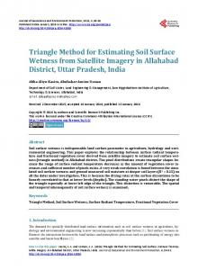
MATERIALS AND METHODS SOIL DATASET The data consisted of 272 samples selected by Gijsman et al. (2002) from a nationally coordinated field study using common procedure and methods detailed by Ratliff et al. (1983) and Ritchie et al. (1987) covering agriculturally dominant regions in 15 U.S. states. The dataset was collected in a joint effort of the USDA Soil Conservation Service and Agricultural Research Service and needed the involvement of a great number of people at many locations. The data were collected with plants in the field and thus are representative of the real crop experience in the field. Measurements were made up to a soil depth of 1 to 1.2 m in 0.10 to 0.15 m depth increments in−situ in cultivated fields. The DUL water content was measured few days after wetting the soil, while the LL was measured after plants stopped extracting water due to death or dormancy as a result of soil water deficit (Ratliff et al., 1983). Field−measured LL and DUL values thus do not consider matric potential. These data covered seven soil orders, 60% of which were Mollisols and Alfisols, included all textural classes apart from sandy clay, and had very limited data in clay, loamy sand, and silt, as shown in the standard soil−texture triangle shown in figure 1 (Brady and Weil, 1999). Major texture classes and sample sizes were silty loam (SIL, 74), silty clay loam (SICL, 47), loam (L, 40), clay loam (CL, 37), sand (S, 29), silty clay (SIC, 17), sandy loam (SL, 10), sandy clay loam (SCL, 9), clay (C, 3), and loamy sand (LS, 1). There were, however, no data for silt (SI) and sandy clay (SC). The ranges of values were: clay 1.2% to 54.4%, silt 0.9% to 86.4%, sand 0.9% to 97.4%, organic carbon (OC) 0.1% to 1.9%, and bulk density (BD) 1.2 to 1.8 g cm−3. Soil samples from the same field locations were analyzed in a laboratory for determining LL and DUL with standard lab methods of −1500 and −33 kPa, respectively. The lab−measured LL and DUL differed significantly from the field−measured data. According to Ratliff et al. (1983), the lab−measured LL overestimated for L, SIC, and C, and underestimated for S, SIL, and SCL. The lab−measured data significantly underestimated DUL for most samples compared to the field−measured data, meaning that the field capacity that plants actually experience is much wetter than the field capacity as characterized in the lab. As a result of the differences in measured LL and DUL, the PESW was also

Silty Clay

Clay Sandy Clay loam clay Sandy clay loam Loam

Sandy loam Sand Loamy sand

Silty Clay loam

Silt loam

Silt

Percent sand

Figure 1. Field−measured dataset including 272 soils with a wide range of textures, as shown in a standard soil−texture triangle (Brady and Weil, 1999).

TRANSACTIONS OF THE ASAE

overestimated by up to 0.063 cm3 cm−3 (mostly SI, SIL, and SICL) and underestimated by up to 0.132 cm3 cm−3 (mostly L, SIL, SICL, SIC, SL, and CL). These errors in estimating field available water−holding limits by using lab−measured data would result in major errors in predicting crop growth and yields. Therefore, we only used the field−measured data in the analysis.

similar and thus our top choice, and its LL and DUL values would be assigned to the target soil. This methodology, illustrated for two attributes, can be extended when a soil has many attributes. Rather than using a triangle with two lengths, some multisided object with sides equal to the number of attributes is used. The distance (di ) is expressed in equation 1 for a case with X attributes: 1/ 2

 X  di =  ∑ Si (Vij − Vtj ) 2   j =1   

THE NEAREST−NEIGHBOR ALGORITHM In a typical situation, a user of a crop or water quality model has soil texture information, such as percent clay, silt, sand, and maybe organic carbon for a specific soil, but the user needs LL, DUL, and PESW to run models for soil water balance simulations. Let’s call the soil for which LL, DUL, and PESW needs to be determined the “target” soil (fig. 2). The NN algorithm searches its memory (the soils database) to see if it has seen this type of soil before in K nearest neighborhoods. It does not have to be an exact match; it just has to be the “best” soil, the closest match. According to Lall and Sharma (1996), in most practical cases, neighborhoods (K) may vary from 1 to N , where N is the total number of soils in the database. The underlying concept of the methodology for a case with K = 1 is illustrated in figure 2. Suppose we want to find parameters for a target soil, which has 20% clay and 60% sand [Target (20,60)]. A search finds four soils in the proximity of Target (20,60): A1 (22,58), A2 (24,54), A3 (20,52), and A4 (22,63). In order to find which soil is closest (because K = 1) to the target soil, their Euclidian distances di (i = 1, 2, 3, and 4) are calculated as the length of the longest side of an imaginary right angle triangle drawn with the hypotenuse from the target to each soil. Using the Pythagorean theorem, the distance (or hypotenuse length) from the target soil to soil A1 is

(1)

where Vtj and Vij are the jth component (such as % clay) of the target (t) and ith nearest neighbor, respectively, and Sj is the scaling weight for the jth component. For example, if the target soil had clay, sand, silt, and OC values of (20, 60, 20, 1.5), then the corresponding A1 might be (22, 58, 20, 1.8), A2 might be (24, 54, 22, 0.8), A3 might be (20, 52, 28, 1.4), and A4 might be (22, 63, 15, 1.4). Running through the calculations with Sj = 1, A1 gives: (a, b, c, d) = (22, 58, 20, 1.8) − (20, 60, 20, 1.5) = 2, −2, 2, 0.3 d1 = a2 + b2 + c2 + d2 2

= 22 + (−2)2 + 22 + 0.32, or d1 = 3.48 Since the magnitude of OC in the dataset is so low relative to clay, sand, and silt, it has virtually no effect on the calculation of distance in the NN approach. Therefore, if OC were to have a similar influence as other variables on distance calculation, it is essential to scale their values. The scaling factors determine the relative importance of different parameters of the training dataset. The scaling factor for an attribute j was calculated by dividing the maximum range (i.e., maximum value − minimum value) among all X attributes in the database divided by the range of attribute j:

(22 − 20)2 + (58 − 60)2

or 2.83. Similarly, A2’s distance is 7.21, A3’s distance is 8.00, and A4’s distance is 3.60. Because A1 has the shortest distance to the target soil, it is the most

65

A 4(22,63)

d4 Target (20,60)

Sand (%)

60

d1

A 1(22,58)

55

d2

d3 A 3 (24,54) A 2 (20,52)

50 15

17

19

21

25

Clay (%) Figure 2. Graphical representation of the nearest−neighbor (NN) method for finding the “best” match for the target soil described using two attributes: clay (20%) and sand (60%). The NN method finds four soils in the neighborhood of Target (20,60). The distances of each of these four soils (A1, A2, A3, and A4) from the target are found using the Pythagorean theorem as 2.83, 7.21, 8, and 3.6, respectively. Because A1 has the shortest distance to Target (20,60), it is the most similar to the target soil and is thus the first choice.

Vol. 47(5): 1437−1444

1439

Sj =

max[range(1), range(2),...range( j ),..range( x )] range( j )

(2)

Using the range of values calculated for clay, silt, sand, and OC for the 272 samples earlier, the scaling factor for clay was: clay = max[(54.4 − 1.2), (86.4 − 0.9), (97.4 − 0.9), (1.9 − 0.1), (1.8 − 1.2)] / (54.4 − 1.2) = 1.81 Similarly, scaling factors for assigning equal importance to silt, sand, OC, and BD were 1.13, 1.00, 54.21, and 166.38. When each scaling factor is multiplied into each attribute (eq. 1), new distances are calculated. The value of LL (or DUL) can be estimated as an appropriate weighted average of the K nearest neighborhoods yi (i = 1, 2, ..., K): ^=

y

N ^   RMSE s = N −1 ∑ (P i − M i ) 2  i =1   N   ^ 2 RMSE u = N −1 ∑ ( Pi −P )  i   i =1

K

∑ wi yi

(3)

i =1

where i = 1 ... K records the indices of the K neighborhoods, yi are the corresponding data (LL or DUL) values, and the weights (wi ) depend on the distances between the target point and the attribute data values of the K nearest neighborhoods. After experimenting with a number of distance−based weighing schemes, we implemented a weight function defined after Lall and Sharma (1996) as: wi =

1 i

(4)

K

1 j =1 j

∑

where i is the rank of neighbors in ascending order (smallest distance to farthest distance). Leave−one−out cross−validation (Lall and Sharma, 1996) was performed on the training dataset. RMSE decreased when some unwanted parameter were turned off and increased when some important parameters were turned off. In this parameter−dropping algorithm, 31 parameters, combining clay, sand, silt, OC, and BD (in combinations of one to five parameters, or nCr where r = 1 to 5) were evaluated by turning off one parameter after another, one at a time. Parameters and K values leading to the lowest RMSE were selected as the best predictors. STATISTICAL PERFORMANCE MEASURES Two statistical indicators used in estimation models are the root mean square error (RMSE) and the mean error (MBE). These were calculated as: N   RMSE = N −1 ∑ ( Pi − M i ) 2  i =1  

0.5

N

MBE = N −1 ∑ ( Pi − M i ) i =1

(5)

where N is the number of data pairs, Pi is the ith predicted value, and Mi is the ith measured value. The MBE provides information on performance of a model. A positive value gives the average amount of overestimation in the estimated val-

1440

ues, and vice versa. The smaller the absolute value, the better the model performance. The RMSE provides information on the performance of a model by allowing a term−by−term comparison of the difference between predicted and measured values. The smaller the RMSE value, the better the model’s performance. However, the RMSE does not differentiate between under− and overestimation. Under the proposition that an estimate depends on measurement and measurement is error free, the average error described by the RMSE can be further portioned (Willmott, 1982) into average systematic (RMSEs ) and unsystematic (RMSEu ) errors (RMSE2 = RMSE2s + RMSE2u ) defined as: 0.5

0.5

(6)

^

where P i = a + b ⋅ M i , and a and b are the parameters associated with an ordinary least−square linear regression between measured (Mi ) and estimated values (Pi ). The magnitudes of RMSEs and RMSEu can be helpful in deciding whether or not a method is acceptable. Ideally, not only should RMSE be low but also, since a good method ought to explain most of the systematic variation in measurements, RMSEs should be relatively small, while RMSEu should approach RMSE. Because RMSE is more sensitive to extreme values due to its exponentiation, it can be considered as a high estimate of the actual average error. To balance such situations, the index of agreement, d (Willmott, 1982), was also used: N   ∑ ( Pi − M i ) 2  i =1 d = 1−  N  ∑ Pi − M + Pi − M   i =1

((

) (

    2   

))

(7)

Ideally d, a unitless measure, should be close to 1. Nevertheless, although these indicators provide a reasonable procedure for model comparison, they do not indicate objectively whether a model’s estimates are statistically acceptable. The t statistic was used to compare methods and at the same time to determine whether the model’s estimates are statistically significant at a particular confidence level. The t statistic can be defined from the MBE and RMSE errors as: t=

(N − 1)MBE 2 RMSE 2 − MBE 2

(8)

It is desirable to have a smaller value of t to ensure better performance of the model. Furthermore, in order for the model’s estimates to be judged statistically significant at a level of significance (a), the calculated t value must be less than the critical t value. The critical t value depends on a and the degrees of freedom (N − 1). The level of significance (a) can vary between 0 and 1, but we chose a value of 0.005 (one−tailed t−test) so that the corresponding critical t value is t = 2.594 for 271 (N − 1) degrees of freedom.

TRANSACTIONS OF THE ASAE

0.070 Clay Clay+Sand Clay+Sand+BD Clay+Sand+OM+BD

RMSE of DUL (cm 3/cm 3) using cross validation

0.065

Clay+Sand+OM Clay+Silt+OM

0.060

0.055

0.050

0.045

0.040

0.035

0.030 0.050

RMSE of PESE (cm3/cm 3) using cross validation

Clay Clay+Sand Clay+Sand+BD

0.045

Clay+Sand+OM+BD Clay+Sand+OM Clay+Silt+OM

0.040

0.035

0.030

0.025

0.020 1

2

3

4

5

6

7

8

9

10

Nearest Neighborhoods

Figure 3. Root mean square error (RMSE) in estimated (a) DUL and (b) PESW using cross−validation method with various combinations of parameters and up to ten neighborhoods.

RESULTS AND DISCUSSION THE NEAREST−NEIGHBOR METHOD After applying the parameter−dropping algorithm using 31 combinations of variables in the original dataset, we found that RMSE between the predicted and observed DUL and PESW for all 272 cases decreased with increasing nearest neighborhoods (or K values) (fig. 3). As K increased, the RMSE vs. K curve became U−shaped, with a fairly broad

Vol. 47(5): 1437−1444

bottom and steep sides (data not shown for large K values); thus, one could really choose any value of K in the range of the broad bottom without compromising the RMSE values. RMSE in LL, DUL, and PESW was reduced as neighborhoods increased to 6, which was chosen as the best K value. RMSE was lowest using clay, sand, and OC as predictors. The only exception was DUL, which can be equally well predicted using clay, silt, and OC. Clay alone was the poorest predictor of all combinations tested, but adding sand to clay

1441

increased the accuracy of LL, DUL, and PESW (RMSE was lowered by 25%, 39%, and 15%, respectively). Incorporating OC into the estimation along with clay and sand had the most dramatic effect, further lowering the RMSE of LL, DUL, and PESW by 10% to 15%. BD along with clay and sand lowered the RMSE of PESW by 17% and that of LL and DUL by 1% to 3%. On the other hand, using OC and BD with clay and sand lowered the RMSE of LL by 7%, DUL by 11%, and PESW by 5%. Implications of these findings for this dataset are that LL and DUL may be estimated with reasonable accuracy using either OC or BD in addition to clay and sand, but PESW is best predicted using clay, sand, and OC. Statistical indicators (MBE, RMSE, d index, and t statistic) for the NN method confirmed that the NN method provides reliable estimates of LL, DUL, and PESW (table 1). Regression analysis of estimated and measured values showed that the intercept was not significantly different from zero for all three parameters (P < 0.05). The slope and P value were, respectively, 0.98 and 0.025 for DUL, 0.96 and 0.001 for LL, and 0.96 and 0.030 for PESW (table 1), suggesting that the estimated values fitted well along the 1:1 line at confidence levels of 97% or higher. The d index of 0.85 and higher and t statistics