AJAE 1(5):188-193 (2010)
ISSN:1836-9448
Dynamic neural network model for identifying cumulative responses of soybean plant growth based on nitrogen fertilizer compositions A. Suyantohadi1,2*, M. Hariadi2, MH. Purnomo2, T. Morimoto3 1
Agricultural Technology Faculty, University of Gadjah Mada, Jogjakarta, Indonesia Electrical Engineering Dept, Institut Teknologi Sepuluh Nopember, Surabaya, Indonesia 3 Biomechanical System Dept, Ehime University, Tarumi, Matsuyama, Japan
2
*Corresponding author:
[email protected]
Abstract In this study, comparison between dynamic neural network and mathematical model was investigated for identifying cumulative responses of soybean plant growth. In this model, cumulative responses of stem diameter and plant height were used as an output factors and fertilizer compositions using nitrogent (N) were used as an input factors. Dynamic neural network was applied to explore and examine the number of data pattern on cumulative responses of soybean plant growth for acceptable identification, through simulation of a given model. The identification cumulative responses of soybean plant growth using dynamic neural network was resulting more performance compared with least square of a mathematical method. Dynamic neural network using time delay in backpropagation algorithm generated best performance in parameter number (n) =1, learning rate (lr) of 10, momentum constant (m) of 0.9 and the limit of error (err) 0.1 for identifying cumulative responses of stem diameter and plant height of soybean plant growth. The techniques obtained here can be applicable to a wide variety of identification problems in plant cultivation systems.
Keywords: dynamic neural network, model, soybean, plant growth. Abbreviations: ARMA_Auto Regressive Moving Average; SISO_Single Input Singgle Output; EA_Error Derivative; EI_Error Quantity; EW_Error Weight; N_Nitrogen; P_Phosphor; K_Potassium. Introduction Modeling of dynamic systems on system identification is one of a tool for model building.( Ljung and Glad, 1994). In the method, a model is built based on the actual input and the output data measured from real systems. Input in system identification modeling has been used to run a simulation program. Simulation can be used for decision making and could be expected to help user in developing and improving the results of an agricultural commodity. Soybean plant growth, is efficient to monitor the physiological responses of the plant and then use it for achieving optimization. The plant growth of soybean is characterized by complexity and uncertainty because is affected by environment factors during the growing in the plantations. Fertilizer factors is the most important conducted the growth of soybean due to easy monitoring. The indicators of soybean plant growth have showed the physiological responses and they could be selected for measuring. Stem diameter and plant height of soybean have been showed the important indicators of plant growth affected by fertilizer used. But, it is not easy to find the identification in this case because the physiological and ecological responses during plant growth, as affected by the environmental factors, are characterized by complexity and uncertainty such as non-linearity and time variation. It is difficult to construct a dynamic model of plant production system using conventional mathematical methods.
These techniques are not suitable for solving the problem. (Bhat et al., 1990). Intelligent approaches have emerged as promising techniques for dealing well with complex systems in plant and biological production systems. An intelligent techniques combining neural networks with genetic algorithms has been developed for realizing the optimization of cultivation and storage processes (Morimoto et al, 2007). Shailendra and Barai (2010) was investigated an attempt to study the learning and predicting capability of neural network models through simulating a complex and highly nonlinear problem. Dynamic system performances on maturity of green peas have been predicted by application of neural networks method (Higgins et al., 2009). Identification system in the development of agricultural technology has been applied by using this method (Morimoto et al., 2005; Suyantohadi et al., 2009; 2010). Artificial neural network have been capable on assessment of agricultural mechanization status of potato production system (Morteza et al., 2010). In this study, the physiological responses as a reaction of changes as affected by environment on soybean plant growth, the black-block neural network diagram of input output relationship has described. The changes of unknown process can then be examined. It is noted that the dynamic neural network model was constructed based on the identification and using observed data related to input and
188
output of process in which the input is environmental factors and the output are indicators of soybean plant growth. The study aims to design dynamic system on physiological cumulative responses such as stem diameter and plant height of soybean plant growth using neural network model with input on the parameters of N fertilizer compositions in the cultivation of soybean plant. The input neural network has identified N fertilizer compositions on the output of the cumulative responses for growing soybean. Results of this research have expected to become the basic to identify cumulative responses of soybean plant growth based on the N fertilizer compositions. Material and methods Plant materials Soybean which was cultivated on greenhouses were used for this experiment. Fertilizer composition was used as N fertilizer. Rahimizadeh et al. (2010) has reported nitrogen fertilizer rates were significantly effected on growth of plants. The other fertilizers such as P and K fertilizers and organic liquid fertilizers were made constant value. Output of neural network has used on N compositions on soybean plants during growth. Soybean plant growth data in this study was designed on the random group with 3 trial experiments at 12 group based on some variance of N fertilizer compositions. Blocks with the size of 1 m x 4 m were used as experiment test for growing soybean cultivation. N compositions fertilizer on 12 group were separated at 9 group at designed on learning of neural network model and 3 group for data of model validation. P and K fertilizer during this study were made constant value with composition 50 kg/ha at 0 days, 50 kg/ha at 10 days, 75 kg/ha at 75 kg/ha days for all of groups. Variable cumulative response parameters during soybean plant growth were observed including stem diameter and plant height. In this study, the other factors such as environment temperature and humidity, that occurred during this study was used as a measurement with no treatments.
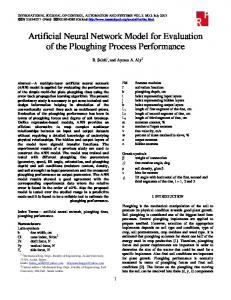
Fig1. Dynamic neural network topology for identifying using timeseries data and time delay
Mathematical model for data acquisition A model was developed to make the process of identification easier, in this study, a mathematical model given by a first order differential equation was used instead of an actual system defined as a dynamic system, and all data for identification were obtained from this model. The model from was given as follows:
x = Ax + Bu , Y = Cx Z
=
fy dt
..........
.......... .......... (1) .........(
2 )
Where x was state variable, u was input variable which corresponds to environtmental factors, y was output variable which corresponds to the rate of plant growth responses, A,B, and C were coefficient factors and here given as -0.9, 0.9 and 1.0, respectively. The output y was called velocity responses. By integrating y, furthermore, the cumulative response z were obtained, as expressed in equation (2). It was assumed that the cumulative responses such as plant growth could be obtained from the output of Z.
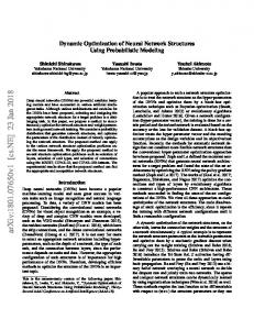
Fig 2. Stem diameter and plant height measuring as affected by nitrogen fertilizer
189
System identification using least square model Agricultural cultivation systems are characterized by nonlinearity, poor initial estimate of the optimal solution, stiffness and uncertainty in model parameters and in-exogenous disturbances. These conditions and characteristics are only be described mathematically by large scale, non-linear, non-steady state, stiff differential or integer differential equation. But, of course, the actual system is mostly non-linear system. In many cases linearization of the non-linear data is conducted. Some methods for this purpose are Auto Regressive Moving Average (ARMA) Model. System identification has been extensively applied to agricultural systems. This method can be applied to unknown process which dynamically characteristics are ill defined and used to describe the dynamic system characteristics. In fact, for system with many input signals and / or many output signals are called multivariable systems, modeling could be difficult. A basic reason for difficulties is that the coupling between several inputs and outputs lead to more complex models. The structures involved are richer and more parameters will be required to obtain a good fit. In this case intelligent approach is more effective for system identification compare to ARMA Model. Let’s we consider a single input single output (SISO) System with unknown parameter ( Fig.2) related with plant growth systems. The input signal is described by u(k) and output signal by y(k) and measurement noise by w(k) that occurs at each sampling time k,k-1,2,...., m (m is data number). Assume that w(k) and u(k) are statistically independent. Then the input-output equation can be presented as follow:
y (k ) =
B ( z −1 ) u (k ) + w (k ) A ( z −1 )
.......... .......( 3 )
Where A(z-1) and B(z-1) are linear mth order polynomials in the backward shift operator z-1(i.e.z-1.y(k)=y(k-1)) which has the following form:
A( z − 1) = 1 + a1z − 1 + ... + amz − m
.......... .......... ( 4 )
This equation means that the output can be estimated from the weight sums of on the m th historical input data. This model is called moving average model and weight parameters are called response or weighting function.
System identification using neural network Neural network is capable of recognizing the relationships between the input and the output of an ill-defined with their own learning ability. Neural network is typically composed of interconnected nodes that serve as model of neurons. Nodes are usually organize into group that called layers that consist of threes layers, i.e.,input layer, hidden layer and output layer (G Liu, et al., 2005). These nodes change all activity modes that they received become output activity and spread it to all nodes in next layer. This conversion process is conducting in two steps. First, each incoming activity multiplied by weight on the connection and added all these weights of inputs to get a quantity that called total output.
X
=
j
y ( k ) + a1 y ( k − 1) + ... + a m y ( k − m ) = b0 u ( k ) + b1u ( k − 1) + ... + bm u ( k − m ) + w( k )
.......( 5)
y ( k ) = − a1 y ( k − 1) + ... − a m y ( k − m ) + b0 u ( k ) + b1u ( k − 1) + ... + bm u ( k − m ) + w( k ).
.......( 6 )
Where e ( k ) = w( k ) + a1 w( k − 1) + ... + a m w( k − m ) Equation above, means that the output y(k) is obtained from historical output data and (m+1) th weight sums of mth historical input data, which is usually called ARMA model. Value of the m is called number of system parameter or system order. On the other hand, more simple expression of the inputoutput relation can defined using the following equation y(k ) = b0u(k ) + b1u(k − 1) + ... + bmu(k − m) + w(k )
.................(7)
y i w ij .......... .......... .....( 8 )
i
Where Xj is total weight input Yi is the activity level of the ith node in the previous layer Wij is the weight of the connection between ith and jth node i is a typical node in the previous layer j is a typical node in the output layer Second, total output will be changed as outgoing activity by a sigmoid function.
Y
=
j
1 1 + e − xj
.......... ......( 9 )
Training a neural network to perform some task, justification of the weight of each node are needed. The purpose is to minimize the differences between actual output and desired output. 1 2
=
E
B ( z − 1) = b 0 + b1z − 1 + ... + bmz − m Substitute of equation (2) and (3) to equation (1), will give an mth order difference equation as follow:
∑
∑
( y
j
− d
j
)
2
..........
..( 10 )
j
Where dj is the desired output of the jth node Yj is the activity level of the jth node in the last layer. Hinton (1992) describe the principle of back propagation algorithm that consists of four steps as follow; Compute how fast the error changes as the activity of an output node is changed. This error derivative (EA) is the difference between actual output and the desired output of the systems that express as following equation:
EA
j
=
∂E = y ∂Y j
− d
d
j
..........
......( 11 )
Compute how fast the error change as the total input received by an output node is changed. This quantity (EI) is the answer from step 1 multiplied by the rate at which the output of a node change as its total input is change.
EI
j
=
∂E ∂ E dy = ∂x j ∂ y j dx
j
= EA j y j (1 − y j )
...( 12 )
j
Compute how fast the error changes as weight on the connection into an output node is changed. This quantity (EW)
190
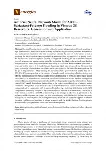
Fig 3. Correlation between nitrogen fertilizer composition and plant growth indicators
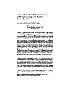
Fig 4. Comparison between estimated from model and observed data EW
ij
=
∂E ∂ w ij
=
∂E ∂x ∂x j ∂w
= EI
j
j
y
j
network could be applied for identification on dynamic system approaches (Morimoto et al., 2005). The characteristic of dynamic system on soybean plant growth consist of: a. Collecting many real data (data sets) that are the time series of nutrient such nitrogen fertilizer as the input variable, the steam diameter and plant height of plant growth as the output variables for the system identifications b. Identifying of steam diameter and plant height of soybean plant growth as affected by nitrogen fertilizer compositions using neural network and then continuing to make a black-box model representative in input – output model for the simulation c. Calculating to identify the responses of soybean plant growth as affected by nitrogen fertilizer compositions at the neural network model for identification. Fig 1. shows a time-delay neural network for dynamic identification. It consists three layer and output data for dynamic identification. The time history of the output y(k) was made by applying time-delay operators (z-1,z-2,.., z-n) to y(k) like y(k-1)= z-1y(k), y(k-2) = z-2.y(k),….,y(k-n) = z–n.y(k) ; where n is the system parameter number which means the number of the past historical data used for prediction. The historical input data on N fertilizer compositions, output data on the cumulative responses of stem diameter and plant height during the development of soybean plant growth are used for the dynamic identifications. Dealing with neural network, three (n+1) th historical input data, {Ur (k),..Ur (k-n)}, {Us (k),..Us (k-n)} and {Up (k),..Up (k-n)}, and two n-th historical output data, {ys (k1),..ys (k-n)} and {ya (k),..ya (k-n)} are applied to the output layer as training signals (k=0,1,..N-n; where N is the data number. The learning method in neural network is an error of back propagation (Hint, 1992; S Janjai, et al., 2009). For predictions, current outputs, ys (k) and ya (k), were estimated from three (n+1) th historical input data, {Ur (k),..Ur (k-n)}, {Us (k),..Us (k-n)} and {Up (k),..Up (k-n)} and two n-th historical output data,.., similar to an ARMA model procedure (Chen, et al., 1990). The most important task for determining the model structure is the choice of the system parameter number n and hidden-neuron number of the neural network. They have been used by trial and error based on cross validations.
....( 13 )
j
is the answer from step 2 multiplied by the activity level of the unit from which connection emanates. Compute how fast the error changes, as the activity of a unit in the previous layer is changed. This crucial step allows back propagation to be applying to multi-layer networks. When the activity of a node in the previous layer changes, it affects the activity of all the output nodes to which it is connect. So to compute the overall effects on the error, we add together all these separate effects on output nodes, but each effect is simple to calculate. It is the answer in step 2 multiplied by weight on the connection to the output node. Fig.1 shows a three layer neural network for identifying the dynamic responses. Let ys(k) and ya(k) (k=1,2,..,N) be the timeseries of plant height and stem diameter of soybean plant growth, respectively. Let ur(k) and us(k) be the time series of potassium dan phospor fertilizer compositions, respectively. As the soybean plant growth measurement, the plant height and stem diameter increased during the stages of growth. Here, increasing of N fertilizer composition was also increased on the both factors. Neural
Results and discussion
For identifying of cumulative responses of soybean plant growth on stem diameter and plant height as an output factors have been affected by N fertilizer compositions as an input factors, collecting data is necessary at the first before designing the model using dynamic neural network. Fig.2 shows the N fertilizer composition related to the soybean plant growth analysis such as for stem diameter and plant height measurement. During 30-days period of soybean plant growth, using variance of N fertilizer compositions, stem diameter and plant height have increased that its shows the characteristic of plant growth. Dariouchy et al. (2009) was used a 7-days period on a time series model of artificial neural network for predicting internal parameters tomato greenhouse. Application neural network training for nonlinear dynamic plants by Muhando (2005) consisting the following properties and capabilies on nonlinearity, supervised learning and adaptivity. Determining the suitable crop rotation for enhancing nitrogen use efficiency of wheat under temperature climate conditions
191
Table 1. Comparison of estimated errors between neural network and least square model in identification of soybean plant growth
Output model Output 1 (Stem diameter) Output 2 (plant height)
Estimated error of identification Neural Network Least Square 0.0035 ± 0.0080 0.0027 ± 0.0004 0.1021± 0.0237
1.1545 ± 0.6432
has been examined by Rahimizadeh et al. (2010). In this study, the correlation between N fertilizer as an input of model and plant height and stem diameter as an output of model has plotted in the diagram. Fig.3 shows the changes of N fertilizer related to stem diameter and plant height. Increasing of N fertilizer has increased both on stem diameter and plant height of soybean plant. The smallest of coefficient correlations on R is shown because the much data was needed. MM Rahman, et al (2009) investigated potentially using N for efficiency and recovery on rice plant cropping systems. In this study, procedure to make identification system has conducted to measure data for the input and the output variables of a system using neural network method. Next, neural network algorithm has been applied in the identification of soybean plant growth is error – backpropagation. Billing et al. (1992) examined artificial neural network available for minimizing the differences between actual output and desired input, such as accelerating the convergence of the back propagation or recursive prediction error routine. One method that usually uses for that purpose on neural network method is back propagation (MM Gupta, et al, 2003). Supervised training algorithm on back propagation consists of two steps, the forward propagation and backward propagation. Step forward propagation and backward propagation is done on the network for each pattern of output measured was given during the network training. Neural network using error-back propagation training method is a rule of generalization delta, includes three stages: 1) the training of feed forward input, 2) calculation and 3) error and adjustment on weight of neurons. During feed forward, every input unit to receive inputs and to continue signaling to the hidden units. Each hidden unit then calculate the activation and signaling to send this to every output. Each unit outputs the activation network to form responses from a given input. Neural network model to identify soybean plant growth parameters consisting of three network layer, which has three inputs, hidden layer and two output layer. Input layer consists of 12 input cell (neuron) in accordance with the number of combination treatment on three input layer. Each hidden layer composed over consecutive 8 and 20 neuron cells. Output layer consists of two neuron cells in accordance with the periodic plant observation data, analysis and components of growth. Architecture design of neural network has been composed on learning rate (lr) of 10, momentum constant (m) of 0.9, the limit of error (err) 0.1. Training on the network was stopped if the value was reached the desired performance after the value of error of performance achieved in the value of 0.1. Performance of an neural network after the training can be measured by looking at the results of the training cross- validation with a set of the testing data input. For cross- validation model, Suhardiyanto, et al, (2009) investigated comparison between estimated from neural network model and observed data from measurement. Testing on model to identify of plant growth using data from nitrogen
each treatment combination of fertilizer has been done to see the performance of neural network design. The data for identification are divided into two independent data sets, as a training data set and a testing data set. The former during modeling designed is used for training the neural network and the latter is used for evaluating the accuracy of the identified model. An equal proportion is desirable for the number of the training and testing data sets. This type of model validations is “Cross-Validations” (Morimoto et al, 2007). Total of measured data is 12 eksperiment in nitrogen fertilizer compositions for mapping relation to input and output variables were divided into nine data set for the data set training network and three data sets for the data set testing network. Nine data sets were selected as the training network and three data set as the testing network for validation model. The model was validated through cross-validation using the testing data sets. Fig 4. shows the comparisons of the estimated stem diameter using neural network model and the observed data measuremen of stem diameter. The identificaion error in the validation data sets were used at 0,1 Similar in the comparison of the estimated plant height using neural network model and the observed data measurement. This showed that the estimated modelling was related with the data observed. Graphical form the results of the training network has been compared to know the accuracy of identification that has been built between the target output data with the output of the test data. System Identification from neural network and mathematical model
To begin with, the data for identification were obtained from the given model by equations (4) and (5) and then divided into two groups: the training data set for building a model and the testing data set for evaluating the accuracy of the model. The training data set, which had nine types of plant growth response patterns and the testing data set which had three types of plant growth response patterns, respectively. Each responses had nine data. Such data number could be seen inadequate for effective identification. The training data set and the testing data set were obtained from the same model but they were independent with each other. Table 1. shows the comparison of estimated error in the identification of the output 1 and the output 2 using neural network and least squares. The unit of each error was a value ten interval days. The system parameter number ( n ) and the hidden neuron number in the neural network were 1 and 5 respectively. Nine type of training data were used for learning neural network model and three type of testing data for this comparison. Here, the minimum value of system parameter numbers n=1 was used for this identification from a view point of computational time saving. In both cases, the estimated errors for the output 1 (stem diameter) were much smaller than that for the output 2 (plant height). This was caused by the output 1 being quite similar to the change of the input pattern. In the condition for the output 1, the estimated error was slightly smaller with the leas squares than with the neural network though both errors showed markedly small values. However, the estimated error for the output 2 was much smaller with the neural network than with the least squares. It is found that the neural network was superior to the least squares for identification of dynamic plant growth. It can be explained that the neural network has the ability to learn and identify any types of data pattern. Using mathematic methods were founded by SL Patil (2009) that investigated neural network auto regressive
192
model performed better than auto regressive moving average model for modeling for tropical greenhouse temperature. Conclusions
In this study, the identification dynamic system of the physiological cumulative responses such as plant height and stem diameter of soybean plant growth during cultivation were carried out by using neural networks. Based on the final resultings, neural network model was concluded that a threelayer neural network with time-delay operators was useful for identifying the dynamic changes in cumulative responses plant height and stem diameter of soybean plant growth, as affected by nitrogen fertilizer composition. Dynamic system of plant growth models using neural network in the mapping for input to output variables could be obtained for implementing in soybean plant. Based on the observed data using fertilizer composition, as affected to the cumulative responses of soybean plant growth as stem diameter and plant height, could be founded for building a model. Using these methods, for identifying cumulative responses stem diameter and plant height on soybean growth could be measured and informed. References
Dariouchy A, Aassif E, Lekouch K, Bouirden L, Maze G (2009) Prediction of the intern parameters tomato greenhouse in a semi-arid area using a time-series model of artificial neural networks. Measurement 42: 456 - 463 Bhat NV, Minderman PA, Avoy TMC, Wang NS (1990) Modeling chemical process systems via neural computation. IEEE Control System magazine 19(3):24-30. Billing SA, Jamaludin HB, Chen S (1992) Properties of neural network with applications to modelling non-linear dynamical systems. International Journal Control 55 (1):193 – 224. Chen S, Billing SA, Grant PM (1990) Non-linear system identification using neural network. International Journal of Control 51(6):1191-1214. Liu G, Yang X, Li M (2005) An artificial neural network model for crop yield responding to soil parameters. Springer-Verlag Berlin LNCS 3498:1017.1022. Higgins A, Prestidge D, Stirling D, Yost J (2009) Forecasting maturity of green peas: An application of neural networks. Computer and Electronic in Agriculture 70:151- 156. Hint GE (1992) How neural network learn from experience. Scientific America 12:105 – 109. Hinton GE (1992) How neural network learn from experience. Scientific American:105-109. Ljung L, Glad T (1994) Modeling of dynamic system. Prentice hall, New Jersey. Gupta MM, Jin L, Homma N (2003) Static and dynamic neural networks from fundamentals to advanced theory. IEEE Press Jhon Willey and Sons. Rahman MM, Amano T, Shiraiwa T (2009) Nitrogen use efficiency and recovery from N fertilizer under rice-based cropping systems. Australian Journal of Crop Science 3(6):336-351 Morimoto T, Ouchi Y, Yoshinouchi M (2005) A neural network model for predicting the quality of Satsuma Mandarin, Journal Jhita 17 (2):90-98.
Morimoto T, Ouchi Y, Shimuzu M, Baloch MS (2007) Dynamic optimization of watering satsuma mandarin using neural network and genetic algorithms. Agricultural Water Management: 1-10. Morteza Z, Mahmoud O, Assodolah A ( 2010 ) Assessment of agricultural mechanization status of potato production by means of artificial neural network modeling. Australian Journal of Crop Science 4(5):372-377 Muhando BE (2005) Application of genetic algorithm in optimization and neural network training for nonlinear dynamic plants. Master thesis Graduate School of Engineering and Science University of Ryukyus, Japan Rahimizadeh M, Kashani A, Feizabadi AZ, Koocheki AR, Mahallati MN (2010) Nitrogen use efficiency of wheat as affected by preceding crop, application rate of nitrogen and crop residues, Australian Journal of Crop Science 4 (5):363368. Janjai S, Intawee P, Tohsing K, Mahayothee B, Bala BK, Ashraf MA, Muller J (2009) Neural network modeling of sorption isotherms of longan (Dimocarpus longan Lour.). Computers and Electronics in Agriculture 66:209–214 Shailendra K, Barai SV (2010) Neural network modeling of shear strength of SFRC corbels without stirrups. Applied Soft Computing 10:135-148 Patil SJ, Tantau HJ, Salokhe VM (2009) Modelling of tropical greenhouse temperature by auto regressive and neural network models. Bio System Engineering 99:423 – 431. Suhardiyanto H, Arif C, Setiawan BI (2009) Optimization of ec values of nutrient solution for tomato fruits quality in hydroponics system using artificial neural network and genetic algorithm, Journal of Science ITB 41B (2):264- 273 Suyantohadi A, Purnomo MH, Hariadi M (2009) Identification of soybean plant growth on statics neural network. Agricultural Technology Agritech, University of Gadjah Mada:16-23. Suyantohadi A, Purnomo MH, Hariadi M (2010) Artificial life of soybean plant growth modeling using intelligence approaches, ITB Journal of Science 42A (1):23-30
193