International Conference
February 10 - 13, 2010
CYBERNETICS AND INFORMATICS
VYŠNÁ BOCA, Slovak Republic
DYNAMIC OPTIMIZATION OF A HYBRID SYSTEM: EMULSION POLYMERIZATION REACTION R. Paulen*, M. Fikar*, M. A. Latifi** *Slovak University of Technology in Bratislava Faculty of Chemical and Food technology e-mail: {radoslav.paulen, miroslav.fikar}@stuba.sk url: http://www.kirp.chtf.stuba.sk ** Laboratoire des Sciences du Génie Chimique CNRS–ENSIC–INPL 1 Rue Grandville, 54001 Nancy Cedex, France e-mail:
[email protected] Abstract: This work deals with the problem of dynamic optimization of an emulsion polymerization reaction in batch reactor. This process can be described as a hybrid system, i.e. dynamic system with both continuous and discrete character. We obtain optimal trajectories of control variable using control vector parameterization (CVP) method. This method translates infinite dynamic optimization problem into finite nonlinear programming (NLP) problem. The NLP computation requires gradient information which we provide using method of adjoint variables. Keywords: Dynamic Optimization, Hybrid Systems, Emulsion Polymerization
1. INTRODUCTION Hybrid models provide better dynamic information of physical phenomena occurring in processes in real world than classical continuous models. As an example of hybrid system we treat emulsion copolymerization reaction of styrene and α–methylstyrene in batch reactor. Emulsion polymerization refers to a unique process employed for some radical chain polymerizations. It involves the polymerization of monomers in the form of emulsions (Odin, 2004). This process has several distinct advantages. The physical state of the emulsion (colloidal) system makes it easy to control the process. Thermal and viscosity problems are much less significant than in bulk polymerization. The product of an emulsion polymerization, referred to as latex, can in many instances be used directly without further separations (Odin, 2004). Approach used to find an optimal control of a plant or process is termed optimal control or dynamic optimization. It encompasses several techniques, which can be divided in two broad frameworks, variational methods and discretization methods. In variational methods, a classical calculus of variations together with Pontryagin's maximum principle (Pontryagin et al, 1964) is applied. These methods address the dynamic optimization problem in its original infinite dimensional form. A big advantage of this is that we are looking for exact solution to problem without any transformations. But it can be disadvantageous in case of more complex systems. Then a discretization plays an important role, since original infinite dimensional problem can be in principle transformed to nonlinear programming (NLP) problem. And there are plenty of solvers capable to solve NLP problems. There also exist a number of methods which can be utilized to generate discretization grid of variables participating in dynamic optimization problem. Sequential discretization and full 1
International Conference
CYBERNETICS AND INFORMATICS
February 10 - 13, 2010
VYŠNÁ BOCA, Slovak Republic
discretization are two classes of these methods. Full discretization represents an approach which takes advantage of states and control discretization (Tsang et al., 1975). Second class, sequential discretization, is based on control discretization. Sequential discretization is usually achieved via control parameterization, (Brusch et al., 1973) in which the control variable profiles are approximated by a sum of basis functions with a finite set of real parameters. These parameters then become the decision variables in a dynamic embedded NLP. Function evaluations are provided to this NLP via numerical solution of a fully determined initial value problem (IVP), which is given by fixing the control profiles. This method possesses the advantages of yielding a relatively small NLP and exploiting the robustness and efficiency of modern IVP and sensitivity solvers. 2. PROCESS MODEL Like in previous works (Gentric et al., 1999), our goal is to produce polymer of prescribed terminal quantity and quality in minimum time. Quantity condition is represented by final conversion of monomer (styrene and α–methylstyrene) and quality condition is described by the final value of number–average molecular weight, weight–average molecular weight or polydispersity index of polymer. Control variable is reactor jacket inlet temperature. Overall process model involves kinetic model, molecular weight distribution model, and reactor temperature dynamics model. It is described by seven first–order nonlinear ordinary differential equations (ODEs) which right hand sides are varying according to one of the three stages of the process.
Kinetic Mechanism The three stages of the process are as follows: 1. In the first stage, free radicals are produced in the aqueous phase by initiator decomposition. They are captured by the micelles swollen with monomer. The polymerization begins in these micelles. This stage, corresponding to particle heterogeneous nucleation (the polymerization rate is increasing), stops when all of the micelles have disappeared. 2. Particle growth occurs during the second stage. Monomer diffuses rapidly from monomer droplets toward the particles, which are saturated with monomer as long as monomer droplets exist. This stage ceases when all of the monomer droplets have disappeared (the polymerization rate is constant). 3. The third and final stage is characterized by the decrease of the monomer concentration in particles; also the polymerization rate is decreasing. The following assumptions are used in the modeling of the kinetic process: Styrene and α-methylstyrene are both hydrophobic monomers; thus, only micellar nucleation is taken into account. Because of this hydrophobic character, the reactions of propagation, transfer to monomer, termination in the aqueous phase, and radical desorption are neglected. Termination in particles is considered to be very rapid compared to radical entry into particles; thus, it can be assumed that no more than one radical is present in each polymer particle (zeroone system). This allows us to write Pj●=N●, where variable Pj● represents number of activated polymers of chain length j and N● represents number of active particles. The maximum conversion rate considered is generally around 65%, so that gelation has not yet occurred. Thus, the gel effect is not included in the model to avoid unnecessary complexity. Coagulation is assumed to be negligible. 2
International Conference
February 10 - 13, 2010
CYBERNETICS AND INFORMATICS
VYŠNÁ BOCA, Slovak Republic
The kinetic mechanism is then written as follows: Initiator decomposition: A → 2R●
Ra = 2f kd A
Particle formation:
R+m→N
Rn = k1 m R●
Initiation:
N + R● → N●
Ri = k2 N R●
Termination:
N● + R● → N
Rt = k2 N●R●
Propagation:
P●+ M → P●
Rp = kp MP N●
Transfer to monomer:
P ● + M → M● + P ●
RtrM = ktrM MP N●
Here A means initiator concentration, R● stands for initiator radical concentration, m represents number of micelles per unit volume, M is global monomer concentration and finally f is initiator efficiency. Variables R and k differing by index of partial reaction of kinetic mechanism denote reaction rates and reaction kinetic coefficients.
Kinetic Model Only the global monomer concentration is described. The depropagation is taken into account by including in the propagation rate constant a factor depending on the α-methylstyrene molar fraction in the initial charge
k p = k p' exp(− a. f MS )
(1)
where a is a constant, fMS is molar fraction of α–methylstyrene at the beginning of a reaction and k’p is the propagation rate constant for styrene homopolymerization. The quasi-stationary state approximation allows calculating the initiator radicals’ concentration R• =
Ra k1 m + k 2 N p
(2)
where Np = N + N● is overall number of polymer particles. Then the rate of particles formation may be written N& p = k1 m
Ra N A k1 m + k 2 N p
(3)
Here NA stands for Avogadro’s number. Like (Harada et al., 1972), we introduce the factor which is similar to effectiveness for the particles relative to the micelles in collecting an initiator radical
ε=
k2 SN A k1 m
(4)
The rate of particle formation is now expressed by R N N& p = k1m a A εN p 1+ SN A
(5)
With the classical hypothesis that the emulsifier molecules are adsorbed in a monomolecular layer on the polymer particles surface, the emulsifier concentration may be written
S = S 0 − k v ( X M 0 ) 2 / 3 N 1p/ 3
(6)
where S0 denotes initial emulsifier concentration, M0 means initial monomer concentration, 3
International Conference
February 10 - 13, 2010
CYBERNETICS AND INFORMATICS
VYŠNÁ BOCA, Slovak Republic
X signifies monomer conversion and
36π M M kv = 2 3 2 ω P (a s N A ) ρ P
1/ 3
(7)
where MM denotes monomer molecular weight, ωP means polymer weight fraction in particles, variable as represents surface area occupied by an emulsifier molecule and ρP stands here for polymer particle density. The rate of monomer consumption is expressed according to M& = − R p = − k p M p
Np NA
n
(8)
with average number of radicals per particle n = 0.5, and monomer concentration in particles Mp which can be expressed as
M p = M pc =
(1 - X c ) ρ M [(1 - X c ) + X c ρ M /ρ P ] M M
(1 - X ) ρ M Mp = [(1 - X ) + Xρ M /ρ P ] M M
X ≤ Xc X > Xc
(9)
there constant Mpc denotes critical monomer concentration in particles, Xc stands for critical monomer conversion and ρM represents monomer density.
Molecular Weight Distribution Model Besides it is important to evaluate the polymer properties. They are linked to the polymer structure and can be described in terms of average molecular characteristics (number- and weight-average molecular weights, polydispersity index, etc.). The used approach is an extension of the tendency model (Villermaux et al., 1984) to emulsion polymerization. According to the kinetic mechanism, the rates of production of the zeroth, first and second order moments of the molecular weight distribution may be written as
Q& 0 = Rt + RtrM Q& = L( R + R 1
t
trM
)
(10)
Q& 2 = 2 L2 ( Rt + RtrM ) where Rt =
Ra n N p S Np +
ε
RtrM = k trM M p L=
Np NA
(11)
n
Rp Rt + RtrM
Variable L denotes kinetic chain length. Once these moments are known, the number- and weight-average molecular weight ( M n and M w ) and polydispersity index (Ip) can be calculated Mn = MM
Q1 Q0
Mw = MM
Q2 Q1
Ip =
Mw Mn
(12) 4
International Conference
February 10 - 13, 2010
CYBERNETICS AND INFORMATICS
VYŠNÁ BOCA, Slovak Republic
Reactor Temperature Dynamics Model In order to achieve temperature control, it is necessary to describe the reactor temperature dynamics. The reaction takes place in a glass stirred tank reactor. Heat control is realized thanks to a cooling fluid circulating in a jacket at constant flow rate. The inlet temperature of the cooling fluid is controllable. Energy balances on the jacket and the reactor contents give the following equations for the reactor and jacket temperature dynamics
UA V∆H T& = − Rp + (T j − T ) mr C p mr C p T& j =
Fj Vj
(T j ,in
(13)
UA −Tj ) − (T j − T ) ρ jV j C p , j
where V and Vj are reactor contents volume and reactor cooling jacket volume respectively, ∆H means polymerization reaction enthalpy, term mrCp represents reactor total heat capacity, constant U means heat-transfer coefficient, A is cooling surface, variables Fj, ρj and Cp,j signify cooling fluid flow rate, cooling fluid density and cooling fluid heat capacity respectively. All the kinetic coefficients are calculated according to Arrhenius law k i = k i , 0 exp(− E j / R T )
(14)
Hybrid Representation of the Process Model Majority of this section uses notation introduced by (Feehery, 1998). Dealing with the hybrid systems of ODEs means dealing with a system of a form
mode S i
x& ( i ) = f
(i )
[
]
nk
∀t ∈ t 0(i ) , t (fi ) , S i ∈ U S k
( x ( i ) , u ( i ) , p, t )
(15)
k =1
n n n (i ) (i ) where x ∈ ℜ x , u ∈ ℜ u and p ∈ ℜ p . Function f(i) is such that f(i) : ℜ nx × ℜ nu × ℜ p × (i)
(i )
n
(i )
(i )
ℜ → ℜ nx . Switching from one stage (mode Sk) to another (mode Sj) occurs when a unique (k ) ( j) ( j) ( j) (k ) transition condition L j ( x& , x , u , p, t ), S j ∈ P is satisfied. Set P(k) contains all possible (i )
(k ) (k ) (k ) (k ) (k ) ( j) ( j) successive stages of mode Sk. Transition function T j ( x& , x , u , x& , x , u , p, t ) determines possible discontinuity in variables participating in model. There is a special case of transition function defined at mode initial time t = t0(k) where
T j( 0) ( x& ( k ) , x ( k ) , u ( k ) , p, t ) = 0 ⇒ x ( k ) (t 0( k ) ) = x0( k )
(16)
Hence that model represented by equations (5), (8), (10) and (13) is strongly nonlinear and hybrid as well (Salhi et al., 2004). Its hybrid character can be expressed as follows:
mode S i
x& (i ) = f ( i ) ( x (i ) , u, p)
where states vector is defined as
[
x T = M , N p , Q0 , Q1 , Q2 , T , T j
[
]
∀t ∈ t 0(i ) , t (fi ) , S i ∈ {S1 , S 2 , S 3 }
]
(17)
(18)
In our case switching between stages passes in order known in advance. So we can define transition conditions as
L(21) ( x& (1) , x (1) , u , p, t ) = 0 ⇒ N p (t ) = N pst L(32) ( x& ( 2) , x ( 2 ) , u , p, t ) = 0 ⇒ X (t ) = X c
(19)
5
International Conference
February 10 - 13, 2010
CYBERNETICS AND INFORMATICS
VYŠNÁ BOCA, Slovak Republic
where constant Npst represents constant number of particles dependent on temperature and initial load in reactor. Note that due to known sequence of stages we can write
t 0 = t 0(1)
t (f1) = t 0( 2)
t (f 2) = t 0(3)
t (f3) = t f
(20)
Transition functions finally can be defined as
T1( 0) ( x& (1) , x (1) , u , p, t ) = 0 ⇒ x (1) (t 0(1) ) = x 0(1) T2(1) ( x& (1) , x (1) , u (1) , x& ( 2) , x ( 2) , u , p, t ) = 0 ⇒ x ( 2) (t 0( 2) ) = x (1) (t (f1) ) ( 2) 3
T
(2)
( 2)
( x& , x , u
( 2)
, x& , x , u , p, t ) = 0 ⇒ x (t ( 3)
( 3)
( 3)
( 3) 0
) = x (t ( 2)
(2) f
(21) )
The rest of this section forms conditions for particular stages of the process. As it was told before, in process second and third stage number of particles stays constant which says that N& p( 2) = N& p(3) = 0 . In the third stage, calculation of variable Mp changes (see equations (9)). This changes also right hand sides of equations (8), (10) and (13) where Mp is present implicitly.
3. PROCESS OPTIMIZATION We obtain optimal trajectories of control variable using control vector parameterization (CVP) method. This method translates infinite dynamic optimization problem into finite nonlinear programming (NLP) problem. The NLP computation requires gradient information which we provide using method of adjoint variables. Our objective is to compute such a control u(t) of the system that will drive system to desired terminal state (some state values are prescribed at final time) at minimum time possible. We can define our optimization problem as tf
min ∫ dt = t f − t 0 u ( t ), p t 0
s.t. x& ( i ) = f
(i )
[
]
( x ( i ) , u , p ) ∀t ∈ t 0(i ) , t (fi ) , S i ∈ {S1 , S 2 , S 3 }
x (1) (t 0(1) ) = x0(1) h( x ( 3) (t f ), u (t f ), p, t f ) = 0
(22)
u (t ) ∈ [u L (t ), u U (t )] p ∈ [ p L , pU ] where initial state vector is defined as
(x )
(1) T 0
= [ M 0 ,0,0,0,0, T0 , T j , 0 ]
(23)
where M0 is amount of monomer (styrene and α–methylstyrene) input to reactor and T0 and Tj,0 are variables which represent initial reactor and cooling jacket temperature. These are parameters p to be optimized. Lower and upper bounds imposed on parameters as well as on controls are signified by superscripts L and U respectively. Terminal state of the reaction is characterized both by quantity and quality terminal conditions, h(x(tf),u(tf),p,tf). Quantity terminal condition means that we desire final conversion of monomer to be X f = X (t f ) = 1 −
M (t f ) M0
(24)
Quality terminal condition is represented by final value of number–average molecular weight, weight–average molecular weight or polydispersity index of polymer and can be computed by 6
International Conference
February 10 - 13, 2010
CYBERNETICS AND INFORMATICS
VYŠNÁ BOCA, Slovak Republic
equations (12). The optimized control u(t) is reactor cooling jacket inlet temperature Tj,in(t).
Optimization Method Equations (21) state that studied system is continuous and the same goes for the adjoint variables. Optimality conditions derived from application of Pontryagin’s maximum principle (Pontryagin et al., 1964) can be then summarized as ∂H ( i ) =0 ∂u
λ&(i ) (t ) = − λ(3) (t f ) =
∂H (i )
S i ∈ {S1 , S 2 , S 3 }
T
∂x ( i ) ∂G ∂x (3)
(25)
T t =t f
where H ( i ) ( x (i ) (t ), λ(i ) (t ), u (t ), p, t ) = F ( x ( i ) (t ), u (t ), p, t ) + λ(i ) (t ) f ( x ( i ) (t ), u (t ), p, t ) T
(26)
is Hamiltonian function and λ is vector of adjoint variables and G is the non-integral part of objective function. We employ CVP method to solve dynamic optimization problem. In first step, control trajectory u(t) is discretized to final number of intervals with constant control uj, where j = {1, . . . , nu} indicates control interval number. The performance index is evaluated by solving an initial value problem (IVP) of the original ODE system, and gradients of the performance index as well as the constraints with respect to the parameters (p and approximations of u(t)) can be obtained by solving either the adjoint equations or the sensitivity equations.
Computing Gradients Accurate gradients calculation is one of the most challenging steps in solving the NLP problem which was derived from original problem (22) using piecewise–constant control uj applied on specified instant of time ∆tj = tj − tj−1. Gradients of objective function J can be computed such that
∂J ∂G = H (3) (t −f ) + ∂t f ∂t f ∂J ∂G = H (i ) (t −j ) − H ( i ) (t +j ) + ∂t j ∂t j
∀j ∈ {1, K , nu − 1}, S i ∈ {S1 , S 2 , S 3 }
∂x (1) T ∂J ∂G = − J p (t 0 ) + λ(1) (t 0+ ) 0 ∂p ∂p ∂p ∂J = J u (t j −1 ) − J u (t j ) ∀j ∈ {1, K , nu } ∂u j
(27)
where ∂H ( i ) & Ju = ∂u ∂H ( i ) J& p = ∂p
S i ∈ {S1 , S 2 , S 3 }
(28)
7
International Conference
February 10 - 13, 2010
CYBERNETICS AND INFORMATICS
VYŠNÁ BOCA, Slovak Republic
Constraint functions can be expressed in form of optimization criterion (Salhi et al., 2004), so that constraint gradients can be found in similar manner like presented in equations (27).
Optimization Algorithm We employ the procedure which can be described in following steps: Step 1: Perform initial guess for values of uj, ∆tj and p. Step 2: Integrate system forward in time. Step 3: Evaluate objective function and constraint functions. Step 4: Integrate system of adjoint equations backward in time. Step 5: Calculate gradients. Step 6: Use NLP solver to obtain new values of variables uj, ∆tj and p. Step 7: If the optimality conditions are satisfied then quit. Else, go to Step 2.
4. RESULTS AND DISCUSION Optimization algorithm proposed in section 3 is implemented using MATLAB and its NLP solver fmincon which solves constrained nonlinear programming problems. Integration is performed using ode45 integrator where 4th order Runge–Kutta numerical integration method is implemented. Optimization problem is solved for different control discretization scenarios. Obtained results are summarized in following table: Table 1: Comparison of different control strategies for desired terminal state: Xf = 0.7,
nu
J[s]
Xf
M n ×10−3
M w ×10−6
Ip
1
5340
0.7
2.0
4.3
2.13
2
5234
0.7
2.0
4.4
2.20
3
4950
0.7
2.0
4.8
2.38
4
4859
0.7
2.0
5.7
2.87
5
4673
0.7
2.0
5.8
2.87
6
4609
0.7
2.0
5.8
2.87
7
4550
0.7
2.0
6.0
3.01
8
4539
0.7
2.0
6.3
3.13
9
4502
0.7
2.0
6.3
3.13
10
4445
0.7
2.0
6.4
3.18
M n = 2×10³
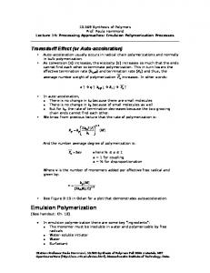
where variable nu represents the number of control segments considered. It can be seen that by the rising number of control segments not only the optimization criterion is lowering its value (as expected) but also an overall quality of polymer produced rises (this can be seen in last two columns of the Table 1). Graphically, the results can be represented in Figure 1 where the control trajectories of selected control scenario with 10 control segments as well as reactor temperature trajectories are depicted. Using of multistart method (i.e. starting algorithm from 8
International Conference
February 10 - 13, 2010
CYBERNETICS AND INFORMATICS
VYŠNÁ BOCA, Slovak Republic
multiple different starting points) showed that optimization problem appears to have multiple local minima. 345 T T
340
j,in
j,in
T,T [K]
335 330 325 320 315 0
0.2
0.4
0.6
0.8
1
time/t
f
Figure 1: Optimal control (Tj,in) trajectory for nu=10
5. CONCLUSIONS We discussed process of copolymerization of styrene and α–methylstyrene. In previous sections we
-
model this process
-
give hybrid representation of process model
-
optimize the process such to produce desired quality polymer in minimum time amount
As the computations suggested there might exist more than one solution to our problem because when the algorithm was launched from different initial point (a multistart method) a different solution was reported at the end of an algorithm run. This suggests that our optimization problem possesses multiple (local) minima. Further this tells that to find an optimal point we should utilize another approach (global optimization) to achieve guarantee of global optimality of control variable profiles. This will be the goal for future works, beside practical implementation of optimal control to real process.
ACKNOWLEDGMENT The authors are pleased to acknowledge the financial support of the Scientific Grant Agency of the Slovak Republic under the grant 1/0071/09. This work was also supported by the Slovak Research and Development Agency under the contract No. VV-0029-07. REFERENCES BRUSCH, R.G.; SCHAPPELLE, R.H. (1973).: Solution of highly constrained optimal control problems using nonlinear programming. AIAA Journal, 11 (No.2), 135-136. FEEHERY, W.F. (1998).: Dynamic optimization with path constraints. PhD Thesis, MIT, Cambridge. FLOUDAS, C.A.; KREINOVICH, V. (2007).: Towards optimal techniques for solving global optimization problems: symmetry-based approach. In Torn, A.; Zilinskas, A.: Models and Algorithms for Global Optimization, Springer, 21-42. 9
International Conference
CYBERNETICS AND INFORMATICS
February 10 - 13, 2010
VYŠNÁ BOCA, Slovak Republic
GENTRIC, C.; PLA, F.; LATIFI, M.A.; CORRIOU, J.P. (1999).: Optimization and nonlinear control of a batch emulsion polymerization reactor. Chemical Engineering Journal, 75, 31-46. HARADA, M.; NOMURA, M.; KOJIMA, H.; EGUCHI, W. (1972).: Rate of emulsion polymerization of styrene. Journal of Applied Polymer Science, 75, 31-46. ODIAN, G. (2004).: Principles of polymerization. John Wiley and Sons, New York, 4th edition. PONTRYAGIN, L.S.; BOLTYANSKII, V.G.; GAMKRELIDZE, R.V.; MISHCHENKO; E.F. (1964).: The mathematical theory of optimal processes. Pergamon Press, New York. SALHI, D.; DAROUX, M.; GENTRIC, C.; CORRIOU, J.P.; PLA, F.; LATIFI, M.A. (2004).: Optimal temperature-time programming in a batch copolymerization reactor. Industrial and Engineering Chemical Research, 43, 7392-7400. TSANG, T.H.; HIMMELBLAU, D.M.; EDGAR, T.F. (1975).: Optimal control via collocation and nonlinear programming. International Journal of Control, 21 (No.5), 763-768.
VILLERMAUX, J.; BLAVIER, L. (1984).: Free radical polymerization engineering – I a new method for modeling free radical homogeneous polymerization reactions. Chemical Engineering Science, 39, 87-99.
10