Dynamic Optimization of SLA-Based Services Scaling Rules Alexandru-Florian Antonescu∗† , Ana-Maria Oprescu‡ , Yuri Demchenko‡ , Cees de Laat‡ , Torsten Braun† ∗ SAP
(Switzerland) Inc., Althardstrasse 80, 8105 Regensdorf, Switzerland of Bern, Communication and Distributed Systems (CDS), Neubr¨uckstrasse 10, 3012 Bern, Switzerland ‡ SNE, Universiteit van Amsterdam, The Netherlands
[email protected], {a.m.oprescu,y.demchenko,delaat}@uva.nl,
[email protected]
† University
Abstract—Current advanced cloud infrastructure management solutions allow scheduling actions for dynamically changing the number of running virtual machines (VMs). This approach, however, does not guarantee that the scheduled number of VMs will properly handle the actual user generated workload, especially if the user utilization patterns will change. We propose using a dynamically generated scaling model for the VMs containing the services of the distributed applications, which is able to react to the variations in the number of application users. We answer the following question: How to dynamically decide how many services of each type are needed in order to handle a larger workload within the same time constraints? We describe a mechanism for dynamically composing the SLAs for controlling the scaling of distributed services by combining data analysis mechanisms with application benchmarking using multiple VM configurations. Based on processing of multiple application benchmarks generated data sets we discover a set of service monitoring metrics able to predict critical Service Level Agreement (SLA) parameters. By combining this set of predictor metrics with a heuristic for selecting the appropriate scaling-out paths for the services of distributed applications, we show how SLA scaling rules can be inferred and then used for controlling the runtime scale-in and scale-out of distributed services. We validate our architecture and models by performing scaling experiments with a distributed application representative for the enterprise class of information systems. We show how dynamically generated SLAs can be successfully used for controlling the management of distributed services scaling.
I. I NTRODUCTION A Service Level Agreement (SLA)[1], [2] is a contract between a consumer and a provider of a service regarding its usage and quality. It defines guarantees or Quality of Service (QoS) terms under which the services are provided, as well as the procedures needed for checking those guarantees. In [3] we presented how SLAs can be used as a control input for a cloud management platform in order to guide both the mapping of distributed services to infrastructure resources, and the dynamic scaling of services based on measured system state parameters. Current advanced cloud infrastructure management solutions, such as OpenNebula [4], VMware vCloud [5] allow the use of scheduling for dynamically changing the number of running virtual machines (VMs). This approach, however, does not guarantee that the scheduled number of VMs will properly handle the actual user generated workload, especially if the user utilization patterns will change. We propose using
a dynamically generated scaling model for the VM bounded services of distributed applications, for adapting the number of VMs as a reaction to the variations in the users’ generated application load. We answer the following question: How to dynamically decide how many services of each type are needed in order to solve a bigger problem within the same time constraints? In this paper we describe a mechanism for dynamically generating SLA bounded scaling rules for controlling allocation of distributed services, by combining data analysis mechanisms with application benchmarking using multiple VM configurations. We extend the Service Middleware Layer (SML) ([2], [3]) developed in EU FP7 GEYSERS [6] project with a new component that brings self-adjusting capabilities to our system. We investigate how SLAs can be dynamically optimized for enhancing the rules controlling the scaling- out and in of services belonging to distributed applications, in particular Enterprise Information Systems (EIS). We describe a mechanism for discovering the dependencies between the service metrics contained in the SLAs. First, we generate allocation profiles for the services of the distributed application and instantiate virtual machines accordingly. Next, we perform a set of benchmarks typical for the application domain, where we continuously increase the number of concurrent EIS requests. Following that, we apply linear regression on the obtained time series in order to learn the dependencies between the different service metrics contained in the SLAs. Finally, we convert the obtained linear models (LMs) into SLA scaling rules, by adjusting the number of distributed service instances according to the value predicted by the LMs. We combine the inter- and intra- analysis on the time series to determine a Pareto set [7] of scaling solutions that cannot be further improved with respect to all features/metrics. The solutions of the Pareto set can be used to create new SLA rules and to schedule SLA actions on distributed applications. We apply a heuristic algorithm for selecting a service scaleout pattern, which is then converted into actual SLA service scale- out and in rules. We validate our models by performing SLA-driven service scaling experiments using a distributed application representative for the enterprise information systems class of applications. We present how time series analysis can be used for
determining dependencies between the services composing the distributed application and how these dependencies can be used for enhancing the SLA rules controlling the application scaling. The rest of the paper is organized as follows. In Section II we shortly describe our previous research concerning the SLA management in distributed cloud environments. In Section III we give a short overview of related work concerning mechanisms for dynamic discovery of services inter-dependencies and service scaling. In Section IV we describe the architecture and functional block of the proposed system. In Section V we present the approach and algorithms used for the dynamic generation of SLA scaling rules. In Section VI we describe the system evaluation. Finally, in Section VII we present our conclusions and future work.
resources such that the SLA is maintained with regards to the agreed amount of virtual resources. This scenario allows us to identify one shortcoming of the GEYSERS environment: how can the operator select the optimum amount of resources allocated to its multi-tenant applications, so that distributed applications will offer the agreed performance levels? For answering this question we implemented the component presented in this paper, Dynamic SLA optimizer (DynSLAOp), which is able (1) to measure the performance increase of a distributed application using an increasing number of service instances, (2) to determine the correlation between the performance indicators of the services composing the distributed application and to use these correlations for calculating a service scaling model and (3) to transform these scaling model into SLA scaling rules.
II. P REVIOUS W ORK
III. R ELATED W ORK We do not consider the variability of the performance of virtual resources for several reasons: first, the cloud providers are constantly improving the isolation mechanisms; second, a large body of work has been dedicated already to this subject; third, the performance is an expected quantity and our estimates have the same property of being observed over a longer time interval. There are multiple frameworks and tools, which allow management of distributed applications composed of multiple interdependent services. One such example is OpenNebula AppFlow [10], which allows definition and management of applications composed of services mapped to one or multiple VMs, enabling automatic VM elasticity management. An important difference between AppFlow and SML is that SML [2] permits definition of distributed application configurations with a variable number of services. Also, SML allows association of SLA-defined application-monitoring states (guaranteed states) by using an extension to USDl-SLA [11]. Gandhi et al. [12] propose a hybrid solution for predicting the data center resource demands using historical monitoring data. They are pro-actively predicting the load, for handling the periodic changes that characterize most cloud utilization patterns. They also propose using a reactive workload demand prediction for capturing the differences from the seasonal workload patterns. We also combine SLA-based control of distributed systems with action scheduling based on previously determined relations between application load and the number of active services. Anh et al. [13] analyze the performance of cloud applications, which share resources with other running applications in the same physical host, by looking at the correlations between application and system performance. We use statistical correlation [14] between the time series corresponding to the performance monitoring metrics of distributed services in order to determine the set of predictors of critical SLA metrics, which can then be used for controlling services scaling.
The GEYSERS project ([6], [8], [9]) provides a novel architecture to leverage the technical advances in networking and IT resource virtualization for multi-provider cloud infrastructure management. This research effort created the Service Middleware Layer (SML) [6] framework for exploring the use of SLAs for automated management of distributed VMbounded services. The SML represents a convergence layer for coordinating IT resources on behalf of various distributed applications. We shortly describe the SML, including its consumption of SLAs during the management of applications and cloud landscape. The GEYSERS architecture [6] consists of three actors, each performing a different functional role: provider, broker and operator. The provider usually owns the virtualizable physical resources (e.g. networks and servers). A provider allows access to its resources by installing the Lower Logical Infrastructure and Composition Layer (LICL) component. The broker component interfaces between multiple providers and operators. This functionality is implemented by the Virtual Infrastructure Provider (VIP), which is managing the Upper LICL component of GEYSERS. The VIP aggregates multiple resources belonging to different providers into virtual resource pools. The operator usually represents the application/user of the composed virtual resources. An operator expresses the expectations and requirements of distributed applications through SLAs. SLAs [2] may contain both (a) consumer-specified service scaling rules and (b) composed application-wide monitoring conditions. In a typical scenario, the Lower LICL discovers its physical resources and informs the broker accordingly. The broker maintains a list of aggregated resources per provider (e.g. total number of CPUs, memory, disks). When asking for resources, the operator receives information about the maximum resources available at each provider and the maximum available bandwidth between the providers (the possibly virtualized optical networks). The operator selects the corresponding provider(s), SLAs are agreed and the VIP manages the selected
IV. DYN SLAO P ARCHITECTURE Intuitively, the new DynSLAOp component answers the following question: How to dynamically decide how many
Application SLA Max. Budget Target Service Metrics
Application Benchmark Trigger
Benchmark Manager
SLA Service Metric Correlation Engine
Distributed Landscape Generator
Multi-variate Regression Model Builder
Multi-Step Scaling Model Builder
Benchmark Store
Service Midleware Deployment
Orchestration
SLA Evaluation Engine
Monitoring
SLA Scaling Engine
Distributed Infrastructure
Fig. 1. DynSLAOp System Architecture
distributed service instances are needed in order to solve the problem of handling a larger workload within the same amount of time it takes to handle a lower workload with a lower number of service instances? To that end, we need to identify the relevant regression parameters in the dependency between problem size, quality metrics and combination of workers (VMs). We then describe the metrics as functions of the number of workers and the workload. We implement a component that dynamically answers the above question by solving newNrWorkers in Eq. 1. A ∗ oldNrWorkers + B ∗ oldWorkload = C ∗ newNrWorkers + D ∗ newWorkload
(1)
The goal of DynSLAOp is to enable the SML to dynamically adjust the number of VMs to the shifting application loads, while maintaining the contract with the user, i.e. the SLA. This is achieved by producing an SLA containing scaling rules for the application services with a variable number of instances, given (1) a semantic representation of the distributed application, (2) the maximum scale-out factor for each service and (3) critical SLA performance indicators. An example of managed distributed application is described in Section VI. The information flow through the DynSLAOp occurs in several stages, and is represented in Figure 1. DynSLAOp takes as input to the Benchmark Manager an SLA with the service descriptions of a distributed application and a critical SLA performance metric along with its critical
threshold. The benchmark manager communicates with the Distributed Landscape Generator for preparing a different number of virtual landscapes composed of different numbers of VMs allocated to each service (within the service cardinality described by the Application SLA). Each virtual landscape contains a monotonically increasing number of VMs. For each distributed landscape, corresponding VMs will be deployed on the physical infrastructure by the Orchestration and Deployment components of the SML, including resolving the configuration dependencies between the VM-hosted services. Once the landscape has been provisioned, the Application Benchmark Trigger will be notified, which will (1) identify the VM holding the generator of application requests, followed by (2) triggering generation of an increasing batch of concurrent user requests (creation of reports based on database queries), until the requests’ average execution time, as reported by SML’s monitoring component, will reach a given critical threshold. The collected monitoring data is stored in the Benchmark Store. Once all the virtual landscapes have been benchmarked, the SLA Service Metric Correlation Engine will begin calculating the correlation coefficients between the time series corresponding to the monitoring metrics defined in the SLA and the time series corresponding to the critical performance metric. The metrics with the correlation coefficient above a given threshold will be selected as the set of predictors for the critical SLA performance metric. The identified set of predictor metrics will then be given to the Multi-variate Regression Model Builder, which will then calculate a linear model for estimating the critical SLA metrics, using the specified set of predictors. Finally, the Multi-Step Scaling Model Builder will take the calculated linear models and will combine them with the information about the number of service instances in the corresponding virtual landscape for calculating a linear model for estimating the number of services in each landscape based on the linear estimation of the critical SLA metric (including the application workload metric - e.g. number of concurrent user requests). The final step consists in selecting a scaling path of virtual landscapes for the distributed application, by applying a heuristic described in Section V and then combining the linear models for the selected virtual landscapes for creating the final scaling models for each service type defined in the application description. The following section describes the algorithms used by DynSLAOp components. V. DYNAMIC GENERATION OF SLA SCALING RULES The generation of the SLA services scaling rules is performed in three phases: 1) application benchmark data collection 2) benchmark data analysis (aggregation and monitoring metrics correlation calculation) 3) application scaling path analysis and service scaling model calculation
A. Data Collection The monitoring information is collected from probes running in each VM. Each probe periodically records the value of a single SLA metric and sends the gathered data at fixed intervals to the monitoring component in the SML. The system observes via the monitoring subsystem both the values for the metrics related to the application load (e.g. the number of requests), and the values indicating the system performance (e.g. query execution time). In order to properly stress the application performance, a benchmark data profile is created containing a snapshot of the monitoring database and the application landscape. This includes all the measured values for the SLA-defined service metrics. The actual application benchmark is packaged within a VM and deployed along with the other VMs of the application. The decision of having the benchmark running on a separate VM was taken in order to ensure the independence of the DynSLAOp framework from the benchmarked application. The DynSLAOp is only aware of the API used for starting the benchmark and for checking its status for determining whether the benchmark has completed. B. Data Analysis The monitoring data for each service instance is aggregated (e.g. averaged) into specified time intervals (e.g. 10 seconds). The data for the same service type is further aggregated, by averaging it. This is done under the assumption that the load is equally distributed between the instances of the same service type. Once the monitoring data has been aggregated, a correlation matrix will be calculated between each time series corresponding to the SLA service monitoring metrics. Starting from the given critical SLA metric, a set is formed from the metrics that are highly correlated (e.g. correlation coefficient higher than 0.7). This is then repeated for each metric in the set. The set of metrics is then added to the benchmark profile, along with (1) the maximum number of concurrent user requests determined by the benchmark and (2) the virtual landscape configuration in terms of VMs per application service. After the benchmark was run on all the application landscapes configurations, the system enters the last phase for determining the services scaling-out model. C. Building the services scaling-out model During this phase, the system will first construct an application ”scaling path” and then will calculate a linear model for estimating the number of services required for achieving the selected maximum performance. The scaling path is composed of a sequence of virtual landscapes able to handle an increasing number of concurrent user requests, while maintaining the defined SLA contracts, as presented in the algorithm below. 1: ScalingP ath = {Lmin } where Lmin is the landscape with the minimal number of service instances of each type 2: SI is the user requests minimum scaling increment 3: V M Dif f erence ← 1
repeat Sel = {} is the set of selected landscapes Llast ← last landscape in ScalingP ath U Rmax ← maximum concurrent user requests(Llast ) for all L ∈ Landscapes do if V M Dif f erence(L, Llast ) < V M Dif f erence AN D maximum concurrent user requests(L) > U Rmax + SI S then 10: Sel ← Sel {L} 11: end if 12: Landscapes ← Landscapes − {L} 13: end for 14: if IS EMPTY Sel then 15: V M Dif f erence ← V M Dif f erence + 1 16: else 17: select optimal landscape from Sel 18: V M Dif f erence ← 1 19: end if 20: until NOT empty Landscapes The optimal landscape is selected by calculating a utility cost function for each landscape and choosing the landscape with the minimum cost value. The algorithm might return multiple scaling paths of equal cost. The maximum common set of predictor metrics is chosen from the selected of benchmark profiles. For each scaling path, using the selected collection of metrics, a larger data set is formed as follows. The aggregated values of the monitoring metrics corresponding to the first landscape in the scaling path are added to the data set. For the next scaling-landscape, the monitoring samples corresponding to the selected aggregated monitoring metrics are chosen such that their timestamps are higher than the time when the concurrent user requests reached the maximum value achieved for the previous landscape. This creates a single data set with an increasing number of maximum supported concurrent user requests. To this data set, the number of service instances in the landscape is added as a new time series. Next, the system computes for each service type a linear model [15] for estimating number of services in the scaling path. Assuming that C is the critical value of the SLA target metric m∗ , mi , i ∈ (1..p) are values of p SLA predictor metrics for mc , vj are number of VMs associated with service Sj , j ∈ (1..s) then 4:
5: 6: 7: 8: 9:
lmk (m1 , m2 , .., mp , v1 , v2 , .., vs ) = Pp Ps α0 + 1 αi mi + 1 βj sj , j 6= k
(2)
Equation 2 defines the linear model lm for estimating the number of service instances of type Sk . The actual SLA scaling rule for service Sk is then written as in Equation 3 SLAout : if lmk > vk then scale-out(Sk ) k SLAin k :
if lmk < vk then scale-in(Sk )
(3)
Equation 3 defines two SLA rules per service type Sk , which continuously monitor the estimated number of service instances lmk and perform either a scale-out, or a scale-in if the required number of VMs for handling current application workload is either greater or lower than the actual number of VMs vk . VI. E VALUATION We have evaluated the DynSLAOp by analyzing the SML behavior when using a DynSLAOp generated SLA for managing a distributed application, representing the enterprise information systems class. We have checked whether the calculated landscape sequence provides a good ”plan-of-attack” and how sensitive it is to the level of difference between the training set (benchmarks generated) and the synthetic workload. The application was tested using a different type of user load, as shown in Figure 2. The number of concurrent requests at successive time moments was given, and the validation application client maintained a number of concurrent requests equal to the interpolated value between the two time moments. For example, if at time t = 0 there should be 10 concurrent requests and at time t = 10 there should be 20 concurrent requests, then at time t = 3 the validation client would maintain a number of 13 concurrent requests. The validation client performs this check every 50ms.
A. Enterprise Information System We consider a general Enterprise Information System (EIS) as the application under study, as this is simple to explain, has high availability and quality of service requirements, involves large data volumes, and is moreover a good representation of the multi-tier, distributed architecture seen in most modern enterprise systems. A typical EIS consists of the following tiers, each contributing to the SLA management problem: consumer, load balancer, business logic and storage layer. Figure 3 provides an overview of the overall EIS topology.
Dynamic SLA Optimizer (DySLAOp)
Service Middleware Platform
Virtual Infrastructure Consumer
Benchmark Consumer
Registry / Messaging
Load Balancer Registry / Messaging
Registry / Messaging
Worker
îðð
Storage
Fig. 3. EIS Topology
Each service is packaged in its own VM along with all necessary supporting software, such as service container and OSGi (Open Service Gateway Initiative) [16] bundles, but also operating system level support scripts, such as boot time initialization scripts and OSGi container start script. The business logic or worker layer contains components that implement the data queries, analysis algorithms, transaction execution and arithmetic processing for the application. Different types of queries, algorithms and arithmetic workloads place different demands on the processing available. They also impact on the end-to-end latency of user requests, such that scaling the size of the CPU and memory available to this layer has a significant impact on the QoS and SLA compliance. There are various benchmarks available, such as Transaction Processing Performance Council (TPC) [17], for creating different transaction or analytics workloads, each generating volumes of data representative of how these EIS applications are loaded in everyday usage. The storage layer provides the interface to resources and mechanisms for creating, reading, updating and deleting data.
ð
ïðð
Registry / Messaging
ëð
Registry / Messaging
îïæíê
îïæìè
îîæðð
îîæïî
îîæîì
Fig. 2. Concurrent Requests Distribution used for SLA validation
While the training data has a clear increasing trend for the number of requests, the same is not true for the actual monitoring data obtained from the virtual machines. Here, the data is being sampled every x milliseconds, leading to difficulties understanding the real state of the system. To this is added the fact that the load is not perfectly balanced across the worker services, leading to the addition of ’noise’ within the observed monitoring time series. In order to level-out the differences between the same service running in different VMs, data aggregation is performed over predefined time intervals (e.g. one minute). This helps taking the decision whether the distributed application performs within the specified SLA contracts.
¹
ðòê
º
ðòì
»
ðòî
¼
ðòð
éððð
ðòè
ëððð
¸
íððð
ïòð
ïððð
·
óðòî
½
ë ïë
íð
ìë
êð
éë
çð
ïðë ïîð ïíë ïëð ïêë ïèð
óðòì
¾
óðòê
¿
¿
¾
½
¼
»
º
¹
¸
Fig. 5. EIS Benchmark response for a landscape configuration with 4 Worker VMs and 6 Storage VMs
·
Fig. 4. Correlogram
As input/ouput storage latency has an impact on the end-toend response time, parallelization and redundancy are used to increase performance and availability. The load balancer redirects requests to appropriate workers based on algorithms and rules, which determine which worker instances are best suited for handling incoming requests. This depends on their current activities, resource consumption and priority of the request. Load balancers can also make decisions about starting and stopping workers in order to free physical processing, memory and storage resources for other activities. This enables more efficient resource management of the underlying resources. As each component, layer and service in the EIS are distributed and autonomous, there is a need for a registration and messaging architecture that coordinates interactions between the distributed components and services. The EIS implementation used in our analysis and development uses (1) the Apache Zookeeper [18] registry and synchronization service for the above mentioned functions, and (2) the Distributed OSGi [19] implementation for transparently exposing the local OSGi services as distributed SOAP [20] services. B. Experimental Setup The following experiments pipeline was executed. • define application as (1) the set of semantic service descriptions, (2) critical SLA metrics and (3) service dependencies and initialization parameters • set maximum service scale-out factor • set SLA range for application response time tr , as an example of a monitored metric for Worker service DynSLAOp outputs the following information: (1) correlogram matrix, (2) the predicted sequence of landscapes, (3) linear regression coefficients, and (4) the final set of regression coefficients associated with this scaling sequence. Finally, the
set of regression coefficients are transformed into SLA scaling rules and the generated SLA is tested as described below. C. Synthetic Workloads for Offline Machine Learning The DynSLAOp Benchmark Manager fires up the workload generator after customizing it for the application agreed during User-SML interaction. The VM containing the benchmark service is used to generate the workload according to four parameters: (1) maximum response time, (2) initial number of requests, (3) concurrent requests increment step, and (4) number of repetitions for each batch of requests. The request generator will perform the following steps: 1) 2) 3) 4)
send the initial number of requests in parallel wait for all requests to complete their execution record the requests’ execution time calculate the average execution time for all the requests in the batch 5) if the average execution time is lower than the maximum specified benchmark response time, then the generator will increase the number of requests and will repeat the procedure from step (1). 6) each batch of requests is repeated for the specified number of times. The correlogram depicting the correlation between all the pairs of aggregated time series corresponding to the EIS monitoring metrics is presented in Figure 4, where each metric is represented by a letter. From this graph it can be observed that metrics belonging to the Load Balancer service (a-e) are highly correlated, together with the aggregated average execution time of the Worker (g) and Storage (l), and the average number of Worker requests. The before mentioned metrics form the actual metrics, which have been used for estimating the linear models for Worker and Storage scaling. For each virtual landscape configuration, the maximum concurrent load, for which the average worker execution time is below 5000ms, is determined. Figure 5 displays the dependency between the concurrent EIS consumer requests
ë
ß½¬«¿´ Ú·¬¬»¼ Ú·´¬»®»¼
ì
îîð
ïêð
î
λ¯«»¬
ïìð
ï
ïèð
í
îðð
ð
ëð
ïðð
ïëð
îðð
îëð
íðð
ïîð
ïðð
ͬ±®¿¹» Í»®ª·½» ʳ
ß½¬«¿´ Ú·¬¬»¼ Ú·´¬»®»¼
í ð
ëð
ïðð
ïëð
îðð
îëð
íðð
Fig. 8. Storage Service Scaling Model
ëððð
ïðððð
ïëððð
expression language, as required by SML. Figure 9 shows the actual application response while the SML was managing the EIS using the DynSLAOp generated SLA scaling rules. The graph of the number of concurrent requests is displayed in Figure 2. The actual VMs scaling for Worker and Storage services is presented in Figure 10, showing both the scaling-out and scaling-in.
ð
and the response time measured at the worker, for a virtual landscape composed of 4 Worker VMs and 6 Storage VMs. The dependency between the maximum number of concurrent user requests and the number of worker and storage service instances is displayed in Figure 6. From the graph can be observed that the request handling capacity of the distributed application stops increasing after a certain point. From the application source code profiling it became clear that the bottleneck was caused by the database connection management at the storage service. The authors think that replacing the current database connection release mechanism with a pooled connection management would increase the application parallelization. However, at the time we performed the experiments, there was no such straightforward implementation for MySQL [21] using OSGi [16]. Figures 7 and 8 show the regression models for Worker, respectively Storage services. Each plot presents the number of VMs for Worker, respectively for Storage services (black line), the regression model fitted values (blue line) and the filtered number of VMs resulting by applying a moving average smoothing combined with truncating the resulting value. In each graph, the blue line represents the model fitted values, while the black line represents the actual number of service instances determined from the scaling path. For the application under test, the maximum request handling capacity was reached for a virtual landscape composed of 4 Worker VMs and 8 Storage VMs. After this point there was no significant increase in application processing capacity, given the requirement of executing the concurrent requests in less than 5000ms. As previously mentioned in Section V-C, the resulting set of regression model coefficients were transformed into an SLA scaling rule, expressed as two IF statements using MVEL [22]
ï
î
Fig. 6. System requests’ handling capacity vs. number of Worker and Storage VMs
ì
ë
èð
ê
é
ɱ®µ»® Í»®ª·½» ÊÓ
è
Fig. 7. Worker Service Scaling Model
îïæíê
îïæìè
îîæðð
îîæïî
îîæîì
Fig. 9. Average Worker Execution Time [ms]
Due to the fact that the service scale-out was triggered when the number of EIS concurrent user requests reached the maximum handling capacity of the application (average request execution time exceeded the maximum execution time), combined with the fact that VM instantiation is not
ê
R EFERENCES
ð
î
The work in this paper has been (partially) funded by the European Union through projects GEYSERS (FP7-ICT248657) and Mobile Cloud Networking (FP7-ICT-318109).
ì
è
ACKNOWLEDGMENT
ɱ®µ»® ͬ±®¿¹»
îïæíê
îïæìè
îîæðð
îîæïî
îîæîì
Fig. 10. Actual Service Scaling
an immediate action (average VM instantiation time was one minute plus around one minute for the OSGi bundles to start and to register to the distributed OSGi registry), the actual average execution time exceeded the SLA defined limit of 5 seconds (plotted as the red line), because of the delay between the VM instantiation time and the moment when the service becomes operational. This situation was repeated several times during the experiment, but only during the ramp-up phase. Towards the end of the experiment there was no SLA breach as the application had enough free capacity. Overall, the experiment was a success, with 84% of the time enforcing the SLA, and a median execution time of 4284ms. VII. C ONCLUSION We have presented a way of dynamically enhancing SLAs by generating SLA-bounded scaling models for the the VMbounded services of the distributed applications. The resulting SLA scaling rules enable a service management system to react to the variations in the number of application users, while minimizing the number of SLA violations, therefore facilitating service scale-out and service-in. We have described the analytic and benchmark mechanisms for dynamically generating the SLA scaling rules. By using heuristics for selecting the appropriate scaling-out paths for the services of distributed applications, we have shown how SLA scaling rules can be inferred and then used for controlling the runtime scale-in and scale-out of VM-bounded services. We have validated our architecture and models by performing scaling experiments with a distributed application representative for the enterprise class of information systems. We have then shown how dynamically generated SLAs can be successfully used for controlling the management of distributed services belonging to a distributed application. As future work we mention using statistical analytics mechanisms, for (a) detecting periodicity patterns in the SLA monitoring data, and (b) including these patterns as triggers of SLA actions. We also mention SLA violation debugging as another motivation for using SLA metrics statistical correlation, in order to find the cause of SLA violations.
[1] W. Theilmann, J. Happe, C. Kotsokalis, A. Edmonds, K. Kearney, and J. Lambea, “A reference architecture for multi-level sla management,” Journal of Internet Engineering, vol. 4, no. 1, 2010. [2] A.-F. Antonescu, P. Robinson, and T. Braun, “Dynamic topology orchestration for distributed cloud-based applications,” in Network Cloud Computing and Applications, IEEE 2nd Symposium on, 2012. [3] ——, “Dynamic sla management with forecasting using multi-objective optimizations,” in Integrated Network Management, IFIP/IEEE Symposium on, May 2013. [4] J. Font´an, T. V´azquez, L. Gonzalez, and R. S. Montero, “Opennebula: The open source virtual machine manager for cluster computing,” in Open Source Grid and Cluster Software Conference, 2008. [5] J. Y. Arrasjid, B. Lin, R. Veeramraju, S. Kaplan, D. Epping, and M. Haines, “Cloud computing with vmware vcloud director,” 2011. [6] E. Escalona and S. Peng, “GEYSERS: A novel architecture for virtualization and co-provisioning of dynamic optical networks and it services,” in Future Network & Mobile Summit (FutureNetw). IEEE, 2011, pp. 1–8. [7] V. Podinovskii and V. Nogin, “Pareto-optimal solutions of multicriteria problems,” Moscow: Sci, 1982. [8] A.-F. Antonescu and P. Robinson, “Towards cross stratum sla management with the GEYSERS architecture,” in Parallel and Distributed Processing with Applications, IEEE 10th Int. Symposium on, 2012. [9] A.-F. Antonescu, P. Robinson, and M. Thoma, “Service level management convergence for future network enterprise platforms,” in Future Network & Mobile Summit (FutureNetw), 2012, 2012, pp. 1–9. [10] “Opennebula appflow,” http://opennebula.org/documentation:archives: rel4.0:appflow, 2013. [11] Leidig, T. and C. Momm, “USDL service level agreement,” http://www. linked-usdl.org/ns/usdl-sla, April 2012. [12] A. Gandhi and Y. Chen, “Minimizing data center sla violations and power consumption via hybrid resource provisioning,” in Green Computing Conference and Workshops (IGCC), Int., 2011, pp. 1–8. [13] A. V. Do and J. Chen, “Profiling applications for virtual machine placement in clouds,” in Cloud Computing (CLOUD), IEEE Int. Conf. on, 2011, pp. 660–667. [14] F. E. Croxton and D. J. Cowden, Applied general statistics. PrenticeHall, Inc, 1939. [15] F. A. Graybill, Theory and applications of the linear model. Duxbury, 1976. [16] O. Alliance, “OSGi-the dynamic module system for Java,” accessed, May, vol. 25, 2009. [17] T. P. P. Council, “TPC-H benchmark specification,” Published at http: // www.tcp.org/ hspec.html, 2008. [18] “Apache zookeeper,” http://zookeeper.apache.org, 2013. [19] “Distributed OSGi,” http://cxf.apache.org/distributed-osgi.html, 2013. [20] F. Curbera and F. Leymann, Web services platform architecture: SOAP, WSDL, WS-policy, WS-addressing, WS-BPEL, WS-reliable messaging and more. Prentice Hall PTR Englewood Cliffs, 2005. [21] “MySQL,” http://www.mysql.com, 2013. [22] M. Brock, “MVEL expression language,” http://mvel.codehaus.org, 2013.