dynamic portfolio optimization using generalized dynamic ... - terrapub

J. Japan Statist. Soc. Vol. 40 No. 1 2010 145–166

DYNAMIC PORTFOLIO OPTIMIZATION USING GENERALIZED DYNAMIC CONDITIONAL HETEROSKEDASTIC FACTOR MODELS Takayuki Shiohama*, Marc Hallin**, David Veredas*** and Masanobu Taniguchi**** We model large panels of financial time series by means of generalized dynamic factor models with multivariate GARCH idiosyncratic components. Such models combine the features of dynamic factors with those of a generalized smooth transition conditional correlation (GSTCC) model, which belongs to the class of time-varying conditional correlation models. The model is applied to dynamic portfolio allocation with Value at Risk constraints on 6.5 years of daily TOPIX Sector Indexes. Results show that the proposed model yields better portfolio performance than other multivariate models proposed in the literature, including the traditional mean-variance approach. Key words and phrases: GARCH model, generalized dynamic factor model, portfolio optimization, Value-at-Risk.

1. Introduction Since the 1995 amendment of the Basel Accord, Value at Risk (VaR) has become the standard criterion for assessing risk in the financial industry. Indeed VaR—defined as the worst loss over a target horizon such that there is a pre-specified probability that the actual loss will be larger—has become the cornerstone risk measure for potential losses. The last decade has witnessed a growing academic and professional literature comparing various ways to determine and measure VaR, especially for large portfolios of financial assets. On the other hand, current practice among institutional investors consists of constructing financial portfolios in two stages. The first stage consists of the asset allocation decision that determines the proportions of the main asset classes, e.g., equity, bonds and cash, in the portfolio. The second stage involves individual asset selection. Most of the methodological efforts aim at optimizing this second stage. Traditional portfolio management theories include the mean-variance analysis of Received March 20, 2010. Revised August 7, 2010. Accepted August 23, 2010. *Department of Management Science, Faculty of Engineering, Tokyo University of Science, Kagurazaka 1-3, Shinjuku, Tokyo 162-8601, Japan. **Institut de Recherche en Statistique, ECARES, Université libre de Bruxelles, CP 114, B-1050, Bruxelles, Belgium, ORFE, Princeton University, CentER, Tilburg University, and ECORE. ***ECARES and Solvay Brussels School of Economics and Management, Université libre de Bruxelles, CP 114, B-1050, Bruxelles, Belgium, and ECORE. ****Department of Applied Mathematics, School of Fundamental Science and Engineering, Waseda University, 3 -4-1, Okubo, Shinjuku, Tokyo 169-8555, Japan.

146

TAKAYUKI SHIOHAMA ET AL.

Markowitz (1952) and the capital asset pricing model (CAPM). The Markowitz efficient frontier represents all portfolios that are efficient in the sense that all other portfolios exhibit smaller expected returns for a given level of risk or, equivalently, higher risk for a given level of expected return. However, a number of studies have raised objections to mean-variance efficiency as the appropriate framework for optimal portfolio selection. The major problem arising from the Markowitz model is the choice of an appropriate measure of risk. The use of the variance as such a measure, which implies that investors are giving equal weights to the probabilities of positive and negative returns, which is ad hoc with the empirical evidence of skewed financial return distributions. Various alternatives to the variance as a risk measure have been proposed. Examples include the mean-semivariance approach by Markowitz (1959), the mean-semideviation models by Konno (1990), and the mean-lower partial moment approach by Bawa and Lindenberg (1977). Often the purpose of the investor is to avoid making large losses at a certain point in the future, that is to say measure risk by the probability that the investment is below the prescribed level at a certain future point. This calls for a mean-VaR approach to portfolio selection. Rockafellar and Uryasev (2000, 2002) proposed the so-called CVaR model, and Campbell et al. (2001) applied a mean-VaR model to US stocks and bounds. Another crucial issue in portfolio management is of a statistical nature, and is related to the size of relevant datasets. The required information is usually scattered through a large or even very large number N of highly interrelated financial time series. Traditional multivariate time series methods, as a rule, are quite helpless in large N . Here also, an alternative methodology is needed. Such a methodology has been developed recently, mainly in empirical macroeconomics, where it has become quite popular, under the name of dynamic factor models. Dynamic factor models allow for disentangling commonness (market return) and idiosyncrasy (stock-specific components). These components are mutually orthogonal (at all leads and lags) but unobservable. A possible characterization of commonness/idiosyncrasy is obtained by requiring the common component to account for all cross-sectional correlations, leading to possibly autocorrelated but cross-sectionally orthogonal idiosyncratic components. This yields the so-called “exact factor models” considered, for instance, by Sargent and Sims (1997) and Geweke (1977). These exact models, however, are too restrictive in most real-life applications, and a “weak” or “approximate factor model”, allowing for mildly cross-sectionally correlated idiosyncratic components, has been proposed (Chamberlain (1983), Chamberlain and Rothschild (1983)), in which the common and idiosyncratic components are only asymptotically (as N → ∞) identified. Depending on the assumptions on the dynamics of the common components, two main types of factor models have been considered in the literature. The static factor models assume that the common components are driven by q factors that are loaded instantaneously. This static approach is the one adopted by Chamberlain (1983), Chamberlain and Rothschild (1983), Stock and Watson (1989,

DYNAMIC PORTFOLIO OPTIMIZATION USING GDFM

147

2002a, b), Bai and Ng (2002, 2007), and a large number of applied studies. The so-called general dynamic model decomposes the common components into q unobservable common shocks and are loaded via one-sided linear filters. That “fully dynamic” approach was developed, essentially, in a series of papers by Forni et al. (2000, 2003, 2004, 2005), Forni and Lippi (2001), Hallin and Liˇska (2007). The static model clearly is a particular case of the general dynamic one. Its main advantage is simplicity, at the expense of a rather severe restriction on the data-generating process, while the dynamic one, as shown by Forni and Lippi (2001), relies on a general representation result and therefore does not place any restriction (beyond the standard assumptions of second-order stationarity) on the data-generating process. In this paper, we consider a conditionally heteroskedastic extension of the Generalized Dynamic Factor Model (GDFM) proposed, under homoskedastic form, in Forni et al. (2000). Both the static and the general dynamic models are receiving increasing attention in finance, where information usually comes under the form of a (very) large number N of interdependent time series. Factor models are at the heart of the extensions proposed by Chamberlain and Rothschild (1983) and Ingersol (1984) of the classical arbitrage pricing theory; they also have been considered in performance evaluation and risk measurement (Chapters 5 and 6 of Campbell et al. (1997)), in the statistic analysis of the structure of stock returns (Yao (2008)), and the analysis of commonness in liquidity (Hallin et al. (2008)). All these articles assume constant volatility. However, if factor models are to be used in finance, it is essential that they incorporate conditional heteroskedasticity. Early examples are Diebold and Nerlove (1989) and Engle et al. (1990), who study single factor models with conditional heteroskedasticity. These models, however, do not belong to the class of static or dynamic factor models considered here. More recently, Alexander (2001), van der Weide (2002) and Barigozzi et al. (2009) consider static and dynamic factor models with conditional heteroskedasticity in the common shocks. Two of the most frequently used multivariate GARCH models are the Constant Conditional Correlation (CCC) and the Dynamic Conditional Correlation (DCC) models of Bollerslev (1990) and Engle (2002) respectively. Silvennoinen and Ter¨ asvirta (2005) propose another way of modeling conditional correlations: the Smooth Transition Conditional Correlation (STCC) model. In this paper we propose a Generalized Smooth Transition Conditional Correlation (GSTCC) model for the idiosyncratic components combined with the GDFM. Therefore, contrary to Barigozzi et al. (2009), heteroskedasticity in our approach is in the idiosyncratic, not in the common component. In practice our procedure is as follows. First we use the GDFM combined with the GSTCC to extract the idiosyncratic components. Second, we compute the VaR of each idiosyncratic component for a given confidence interval (1% or 5%). Third, we construct the portfolio based on the idiosyncratic components and optimize it with respect to the portfolio weights by minimizing the portfolio VaR. Considering the idiosyncratic components instead of the returns for the

148


portfolio optimization is non standard and requires some explanation. The market risk, estimated through the common component, is not diversifiable and the number of assets, though large, is limited. Therefore, minimizing the risk of the portfolio is, in some sense, equivalent to minimizing the risk entailed by the idiosyncratic risks. But since the idiosyncratic components are not observed, they have to be estimated and hence the results may be affected by the choice of the model to disentangle the returns between the market and the stock specific components. It is at this point that GDFM becomes the appropriate tool. GDFM is not, in fact, a model but a canonical representation of the panel under study; this is why it is often called the dynamic factor representation. Contrary to other dynamic factor methods, GDFM methods do not impose any restriction (beyond second-order stationarity) on the actual data-generating process. In other words, if the panel of returns is second-order stationary, then the GDFM is a unique representation. We apply the above procedure to the dynamic optimization a portfolio formed by all the Sector Indexes of TOPIX (the Tokyo Stock Exchange Index). To measure the performance of all the specifications, we do a one-step-ahead out-of-sample exercise. Among all the conditional covariance specifications, the more general model—the GSTCC with the skewed-t distribution—provides the better performance when compared with other specifications and the classical Markowitz mean-variance approach. We also find that the 5% VaR level constraint produces better portfolio performances than the 1% VaR level, as the later has more variability than the former. The paper is organized as follows. Section 2 presents the methodology, with emphasis on the GSTCC model and its implications in mean-VaR analysis. Section 3 describes the dataset under study and presents the results. Section 4 concludes. 2. Methodology Throughout, we consider a N -variate risky asset return series that has been recorded over a time period of length T (we assume that there is no risk-free asset). Let Rit be the observation made at time t for stock i, i = 1, . . . , N , t = 1, . . . , T . This observation is a finite realization of a double-indexed stochastic process {Rit ; i ∈ N, t ∈ Z}. Let ω = (ω1 , . . . , ωN ), ωi ≥ 0 the set of portfolio weights (we do not allow for short selling) such that N i=1 ωi = 1. Denote by ΣN (θ) the N × N spectral density matrix of the N -dimensional vector process {Rt := (R1t , . . . , RN t ) ; t ∈ Z}, and assume that, for all N ∈ N, k ∈ {1, . . . , N } and some ck > 0, supθ (ΣN (θ))kk ≤ ck . For any θ ∈ [−π, π], let λN,k (θ) be ΣN (θ)’s k-th eigenvalue in decreasing order of magnitude. Denote by q the number of diverging such eigenvalues, that is, define q := min{k ∈ N : supN λN,k (θ) < ∞, θ − a.e.} − 1, and assume that q < ∞. Theorem 2 in Forni and Lippi (2001) establishes the existence of a unique decomposition of Rit into (2.1)

Rit = µi + χit + ξit = µi + bi1 (L)u1t + bi2 (L)u2t + · · · + biq (L)uqt + ξit ,


149

where χit and ξit are mutually orthogonal at all leads and lags, ut := (u1t , . . . , uqt ) is q-dimensional orthonormal white noise, bi (L) := (bi1 (L), . . . , biq (L)) is a vector of square-summable filters, and µi is the mean of Rit . This representation is called a dynamic factor representation of Rit ; the χit ’s are the common, and the ξit ’s the idiosyncratic components, respectively, of Rit . An important problem is to determine the number of common shocks q. To do this, we use the Hallin and Liˇska (2007) procedure for the identification of the number of dynamic factors. This procedure consists in tuning the penalty term of an information-theoretical criterion by a positive factor c until some stability in the identification is reached. ˆ N (θ) be a periodogram-smoothing estimate of ΣN (θ). More precisely, let Σ The reader should keep in mind that henceforth the estimates are a function of T . Based on a panel of N T observations, this estimate is defined as T −1 ˆ N (θ) := 2π ˆ θ − 2πT Iˆ N 2πt , Σ W T T T t=1

where 1 Iˆ N (λ) := 2πT

T −1

T −1 R∗t exp(−iλt) Rt∗ exp(iλt)

t=1

t=1

and ∞

ˆ (λ) := W

W (BT−1 (λ + 2πj))

j=−∞

with a positive even weight function W (λ) and a bandwidth BT . Here R∗t := t −1 ˆ t with µ ˆ t := (ˆ Rt − µ µ1t , . . . , µ ˆN t ) and µ ît = t j=1 Rij . The stochastic ˆ N j (θ) of the estimated information criterion is defined in terms of the eigenvalues λ ˆ spectral density matrices ΣN (θ) , as N T −1 1 ˆ 1 ˆ λN j (θ ) + ckp(n, T ), IC N (k; c) := N T −1 j=k+1

0 ≤ k ≤ qmax ,

c > 0,

=1

where θ := 2π/T for = 1, . . . , T − 1, p(N, T ) is a penalty function such that −1/2

p(N, T ) = (min[N, BT2 , BT T 1/2 ])−1 log(min[N, BT2 , BT 1/2

T 1/2 ])),

and qmax is some predetermined upper bound. For given N and T , let ˆ N (k; c). qˆN (c) := argmin0≤k≤qmax IC A value c0 of c is then determined for which the sequence qˆN (c), as a function of N , exhibits a stable behavior, and the number of factors q is identified as qˆN (c0 ).

150


Once q has been identified, Forni et al. (2000) show how the common and idiosyncratic components χti and ξti can be consistently reconstructed from the observed returns, which we denote by χ ˆti and ξˆti . Experience shows that, even after estimating the common component in the GDFM model appropriately, there still remain significant correlations in the idiosyncratic components. Financial empirical evidence also suggests that the idiosyncratic components show a highly heteroskedastic behavior. Hence we use a multivariate GARCH model for the idiosyncratic part of the panel. The above results on the homoskedastic GDFM and the Hallin and Liˇska (2007) identification method remain valid under conditional heteroskedasticity as fas as the unconditional second-order stationarity holds. Once we have estimated the common component in the GDFM model χ ˆt , ˆ ˆ we obtain an estimated idiosyncratic component ξ t . We assume that ξ t is conditionally heteroskedastic and of the form 1/2 ξˆt = H t z t ,

where the N × N matrix H t = [hijt ] is the conditional covariance matrix of ξˆt , and z t is an iid vector processes such that Ez = 0 and Ezz = I. This defines the standard multivariate GARCH framework where each of the univariate idiosyncratic processes has the specification ξît = hit zit . The conditional variance hit is specified as three different univariate GARCH-type equations under the appropriate non-negativity and stationarity restrictions: the GARCH(1, 1) of Bollerslev (1986), the threshold GARCH(1, 1) or GJR(1, 1) of Glosten et al. (1993), and the APARCH(1, 1) of Ding et al. (1993): 2 hit = ω + αξit−1 + βhit−1 − 2 hit = ω + (α + φDit−1 )ξit−1 + βhit−1

hδit = ω + α(|ξit−1 | − φξit−1 )δ + βhδit−1 , − where Dit−1 is a dummy variable that equals one if ξît−1 is negative, and zero otherwise. The GJR and APARCH models include the leverage effect to account for the well known stylized fact that bad news causes more volatility than good news. Next we turn to specify the correlations. A class of correlation models is based on the decomposition of the covariance matrix into conditional standard deviations and correlations. The simplest multivariate correlation model is the CCC of Bollerslev (1990): H t = D t P D t = ρij hit hjt , (2.2) 1/2

where D t = diag H t and P = [ρij ] is positive definite with ρii = 1, i = 1, . . . , N . The off-diagonal elements of P are defined through the constant correlations of zit and zjt . The CCC model is in many respects an attractive parametrization, but empirical studies suggest that the assumption of constant


151

conditional correlations may be too restrictive. Engle (2002) introduced the DCC model: H t = Dt P t Dt , where D t is defined as above. The conditional correlation matrix P t is P t = (diag Qt )−1/2 Qt (diag Qt )−1/2 where ˆ + A (ˆ ˆ t−1 ) + B Qt−1 , z t−1 z Qt = (ii − A − B) R and where i is the vector of ones, is the Hadamard product (elementwise matrix ˆ it is the i-th standardized ˆ 1t = (ˆ zt , . . . , zˆN t ), and zît = ξît /h multiplication), z residual. The matrices of parameters A and B are N × N diagonal with typical ˆ is the elements αii ≥ 0 and βii ≥ 0 and satisfying αii + βii < 1. The matrix R unconditional correlation matrix that can be estimated as the sample correlation ˆ t . The model becomes the CCC model when A = 0 and B = 0. of z Another class of models allows the dynamic structure of the correlations to be controlled by an exogenous variable, which may be either observable, latent, or a combination of both. One of these models is the Smooth Transition Conditional Correlation (STCC) model of Silvennoinen and Ter¨ asvirta (2005): (2.3)

P t = (1 − G(st ))P 1 + G(st )P 2 ,

where P 1 and P 2 (P 1 = P 2 ) are positive definite correlation matrices that describe the two states of the correlations, and G(·) : R → (0, 1) is a monotonic function of an observable transition variable st ∈ Ft−1 . The most common specification for G(·) is a logistic function G(st ) = (1 + exp(−γ(st − c)))−1 . The parameter γ > 0 determines the velocity of the transition and c its location. The transition variable st is chosen by the modeler to suit the application at hand. We use the common factor estimated from the GDFM. A generalization of this model is the generalized smooth transition conditional correlation (GSTCC) model in which the parameters γ and c are vectorized: (2.4)

P t = V {(I N − G(st ))P 1 (I N − G(st )) + G(st )P 2 G(st )}V ,

where V = {(I N − G(st ))2 + G(st )2 }−1/2 , and G(st ) = diag((1 + e−γ1 (st −c1 ) )−1 , . . . , (1 + e−γN (st −cN ) )−1 ). Note that, if G(st ) = 0, i.e. when the model involves no transition, and P 2 = P 1 , it reduces to the CCC model. We estimate these models under three multivariate distributional assumptions: Gaussian, Student-t with tail index ν, and the skewed-t of Bauwens and

152


Laurent (2005), which is based on the univariate skewed-t of Fernandez and Steel (1998), with tail index ν and skewing parameter ζ. The Gaussian distribution is the benchmark widely used in financial practice. The Student-t is often used to account for the fat tails often found in financial returns, and the skewed-t, less used in practice, features both heavy tails and skewness. The three distributions are labelled n, t, and st, respectively. Therefore, the specifications are referred to as GARCH-n, GJR-n, APARCH-n, and so on. Conditional on past information, the log-likelihood function is constructed for each of the three distributions, and maximized with respect to the parameters. The asymptotic theory for such estimators is quite involved and much beyond the scope of this article; we suggest it as an avenue for further investigation. For the Gaussian distribution, the one-step-ahead VaRt (τ ) is given by hit z(τ ) with z(τ ) being the τ %-quantile. Similarly, for the Student-t distribution, the VaR is given by hit stν (τ ), with stν (τ ) being the τ %-quantile for the standardized Student distribution with estimated degrees of freedom ν. Lambert and Laurent (2000) show that the quantile function skstν,ζ (τ ) of a non standardized skewed Student density is ⎧ α

1 1 2 ⎪ ⎪ if α < ⎨ ζ stν (τ ) 2 (1 + ξ ) 1 + ξ2 skst∗νζ (τ ) = 1−α 1 ⎪ ⎪ ⎩−ξstν (τ ) if α ≥ . (1 + ξ −2 ) 2 1 + ξ2 The τ %-quantile of a standardized skewed-t distribution is skstν,ζ (τ ) =

skst∗ν,ζ (τ ) − m s

,

where m and s2 are the mean and the variance, which depend on the skewing parameter ζ: √ 1 Γ((ν − 1)/2, ν − 2) √ ζ− m= ζ πΓ(ν/2)

and

2

s =

1 ζ + 2 − 1 − m2 . ζ 2

The VaRt (τ ) for a long position is thus hit skstν,ζ (τ ). Once the individual VaRs are computed, the portfolio optimization is done by constructing the portfolio VaR, denoted by VaRN t (τ, ω). Theone-step ahead VaR for a level τ % of the portfolio is defined as VaRN t (τ, ω) = ω H t+1 ωq(τ ), where q(τ ) is the τ % quantile of a generic distribution (z(τ ), stν (τ ) or skstν,ζ (τ )). A set of portfolio weights ω ∗ belongs to the mean-VaR boundary at the τ % confidence level if and only if ω ∗ solves the problem minω VaRN t (τ, ω) subject to ωi ≥ 0, N i=1 ωi = 1 and a given mean level. A dynamic optimal portfolio is constructed by solving every day during the out-of-sample period. 3. Empirical results We consider the Tokyo Stock Exchange market indexes and construct daily out-of-sample portfolio allocations. We compare the results among the vari-


153

Table 1. TOPIX Sector Indexes composition.

No.

Sector

No.

Sector

1 2 3 4 5 6 7 8 9 10 11 12 13 14 15 16 17

Fishery, Agriculture & Forestry Mining Construction Foods Textiles and Apparels Pulp and Paper Chemicals Pharmaceutical Oil and Coal Products Rubber Products Glass and Ceremics Products Iron and Steel Nonferrous Metal Metal Products Machinery Electric Appliance Transportation Equipment

18 19 20 21 22 23 24 25 26 27 28 29 30 31 32 33

Precision Instruments Other Products Electric Power and Gas Land Transportation Marine Transportation Air Transportation Warehousing and Harbor Transportation Information & Communication Wholesale Trade Retail Trade Banks Securities and Commodities Futures Insurance Other Financing Business Real Estate Services

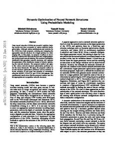
ous specifications for the conditional covariance matrix along with the standard Markowitz mean-variance approach. We use daily log-returns of the TOPIX (Tokyo stock price index) Sector Indexes. They are formed by splitting the constituents of TOPIX into 33 categories. The composition is summarized in Table 1. The sample period goes from January 4, 2001 to June 29, 2007 with T = 1597 days and N = 33 industries. The in-sample period covers 1097 days, from January 4, 2001 through June 22, 2005. The out-of-sample period covers 500 days, from June 23, 2005 through June 29, 2007. Descriptive statistics of the full sample are given in Table 2. There are no statistically significant positive or negative average returns and a great deal of heterogeneity in the standard deviations, ranging from 0.887 for the Foods sector and 2.535 for the Securities and Commodities Futures sector. Skewness is also present in most of the sectors, with 5 showing positive asymmetry and 18 negative at the 10% level. The excess kurtosis is always positive, evidencing fat tails. The Ljung-Box tests reject the null hypothesis of no serial correlation of returns at lags 4 for 21 industries at 5% significant level. While Construction, Food, and Metal Products have relatively strong autocorrelations, Mining, Textile and Apparel, and Fishery, Agriculture, and Forestry do not show significant autocorrelations. To find out the number of shocks in the common component, we apply the Hallin and Liˇska (2007) information criterion. Identification of qˆN is based on a visual inspection of a double plot of the type shown in Figure 1. That double plot provides a measure (an empirical variance S(c) , dotted line) of the instability of the selection qˆN (c) associated with various values of the tuning constant c, along

154

TAKAYUKI SHIOHAMA ET AL. Table 2. Descriptive statistics. SD

Skewness

Excess Kurtosis

LB(4)

TOPIX

Sector

Mean 0.020

1.209

−0.256∗∗∗

4.692∗∗∗

9.723∗∗

Fishery, Agriculture & Forestry

0.030

1.218

−0.143∗∗

5.358∗∗∗

8.722∗

13.162

7.147

11.647

∗∗∗

Mining

0.060

1.912

Construction

0.023

1.385

−0.285∗∗∗

5.071∗∗∗

22.523∗∗∗

25.137∗∗∗

Foods

0.030

0.887

−0.207∗∗∗

5.820∗∗∗

30.267∗∗∗

32.093∗∗∗

∗∗∗

∗∗∗

Textiles and Apparels Pulp and Paper Chemicals Pharmaceutical Oil and Coal Products Rubber Products Glass and Ceremics Products

0.222

∗∗∗

LB(8) 12.363

4.323

0.038

1.284

−0.383

5.459

6.708

−0.008

1.494

−0.050

4.109∗∗∗

7.171

11.711

0.031

1.206

−0.285∗∗∗

5.121∗∗∗

8.923∗

0.010 0.057 0.060 0.034

1.132 1.639 1.606 1.549

0.067

5.557

5.503

−0.030

4.126

−0.209

∗∗∗

−0.167

∗∗∗

6.341 4.188

∗∗∗ ∗∗∗ ∗∗∗ ∗∗∗ ∗∗∗

17.234 19.105

23.394∗∗∗

∗∗∗

20.326∗∗∗

4.179 11.226

13.673∗

∗∗∗

4.489 ∗∗

13.531∗

Iron and Steel

0.107

1.785

−0.045

4.254

Nonferrous Metals

0.013

1.841

−0.144∗∗

4.036∗∗∗

17.690∗∗∗

19.862∗∗

Metal Products

0.044

1.298

−0.213∗∗∗

5.090∗∗∗

17.695∗∗∗

21.612∗∗∗

∗∗∗

∗∗∗

∗∗∗

18.599∗∗

∗∗

15.962∗∗

Machinery Electric Appliances

0.055 0.002

1.388 1.584

−0.372 0.109

∗

Transportation Equipment

0.048

1.437

−0.063

Precision Instruments

0.045

1.428

−0.123∗∗

4.619 4.311 5.416

∗∗∗

∗∗∗ ∗∗∗

3.124

13.885 11.387

6.921

14.560∗

5.283

4.261∗∗∗

4.139

8.755

5.509∗∗∗

4.933

10.743

Other Products

0.032

1.313

−0.227

Electric Power and Gas

0.030

0.929

−0.105∗

6.158∗∗∗

10.106∗∗

22.669∗∗∗

Land Transportation

0.020

1.117

0.049

4.574∗∗∗

14.961∗∗∗

21.012∗∗∗

Marine Transportation Air Transportation Warehousing Information & Communication

0.101

1.892

−0.131

∗∗ ∗∗∗

−0.019

1.624

−0.237

0.052

1.403

−0.025

−0.022

1.936

8.654

∗∗∗

5.154∗∗∗

0.050 −0.287

5.001

∗∗∗

5.336 ∗∗∗

∗∗∗

15.679

∗∗∗

20.339∗∗∗ 10.525

∗∗

24.366∗∗∗ 16.882∗∗

0.056

1.575

Retail Trade

0.005

1.414

0.106∗

5.217∗∗∗

16.963∗∗∗

19.205∗∗

Banks

0.009

1.849

0.111∗

4.952∗∗∗

38.147∗∗∗

38.755∗∗∗

∗∗∗

∗∗∗

33.033∗∗∗

∗∗

14.206∗

0.011

2.356

0.036

3.862 ∗

Insurance

0.050

1.744

0.116

Other Financing Business

0.007

1.758

−0.104∗

Real Estate Services

0.073 −0.028

1.888 1.398

0.096 −0.122

4.906

27.268 10.583

8.696

4.611∗∗∗

23.799∗∗∗

26.667∗∗∗

∗∗∗

∗∗∗

43.074∗∗∗

∗∗∗

31.439∗∗∗

4.045 ∗∗

∗∗∗

7.777

20.066∗∗

Wholesale Trade

Securities and Commodities Futures

4.830

∗∗∗

17.880∗∗

5.997

5.020

∗∗∗

39.601 27.415

Note: The symbols ∗, ∗∗, and, ∗ ∗ ∗ donote statistically significant at 1%, 5%, and 10% level, respectively. SD is the standard deviation of the returns. LB(4) and LB(8) are the Ljung-Box test statistics based on the first 4 and 8 lags of the returns, respectively.

with the final selection qˆN (c) associated with the same value of c (solid line). The procedure then consists in spotting the second interval (starting from the left) of c values over which the dotted line touches the horizontal axis (hence, the value (c) = 0); the number of factors to be selected then is obtained by reading, on the solid line curve, the corresponding value of qˆN (c).

155

20


0

5

10

15

q(c) Sc

0.0

0.2

0.4

0.6

0.8

1.0

c Figure 1. Hallin and Liˇska plot for determining the number of factors.

Figure 1 leads to a selection of one factor and Figure 2 shows the proportions explained by the common components for each industry. Numbers on the horizontal axis correspond to the 33 sectors according to the classification in Table 1. There is heterogeneity across sectors, with a minimum of explained variance of 20% for Electric Power and Gas, and a maximum of 80% for Machinery. On average the common component explains 65% of the total variation. The performance of the idiosyncratic VaR is assessed with a specification test. Specification tests in a quantile based framework are based on failure rates, that is the percentage of times that the realization of the idiosyncratic components are below the VaR. If the model is well specified, its failure rate should be equal to the VaR level. The Christoffersen (1998) likelihood ratio test of unconditional coverage is based on this idea. Let It be a hit variable that takes value 1 if there is a success, that is if the idiosyncractic component is bigger than the fitted VaR, and 0 otherwise: 1, if ξît > VaRt (τ ) It = (3.1) 0, otherwise. If T is the in-sample size, T1 = Tt=1 It is the number of successes and T0 = T −T1 the number of failures. The empirical failure rates can be computed as fˆ = T0 /T


0.0

0.2

0.4

0.6

0.8

156

1

3

5

7

9

11

13

15

17

19

21

23

25

27

29

31

33

Figure 2. Explained variances by a common factor.

and the test statistic is (3.2)

LRuc = −2 log

(1 − τ )T0 τ T1 (1 − fˆ)T0 fˆT1

∼ χ21 ,

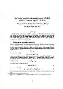
where the null of the test is f = τ . Tables 3 and 4 show the specification test results for τ = 0.05 and τ = 0.01, respectively. Figures 3 and 4 provide, for comparison purposes, the box plots among the different models and distributions. On average, GJR-t produces the most accurate one-step-ahead VaR forecast at the 5% level, followed by APARCH-t. For α = 1%, the horserace winner is again the GJR-t followed by the GJR-st. The Gaussian GARCH models overestimate the VaR at 5% and clearly underestimates it at 1%, as a consequence of the thin tails. The GJR and APARCH models have better performances compared with the GARCH model, which suggests the existence of a leverage effect. This result dovetails with Brownlees et al. (2009). They show that, among a battery of the most common used GARCH models, the threshold GARCH is most often the best forecaster. We construct 500 daily out-of-sample portfolio allocations based on the conditional covariance one-step ahead predictions of the multivariate GARCH models, and we compare the results with those of the Markowitz’s mean-variance model. Given the above specification tests of the VaR, we restrict ourselves to the APARCH and GJR models for the conditional variances. Since the parameters of the multivariate GARCH models change slowly from one day to another, they are re-estimated every 10 days (or two weeks).

GARCH-n 0.0429 0.0356 0.0547 0.0566 0.0538 0.0511 0.0557 0.0438 0.0429 0.0493 0.0566 0.0484 0.0575 0.0365 0.0575 0.0502 0.0456 0.0520 0.0511 0.0420 0.0420 0.0429 0.0383 0.0474 0.0420 0.0566 0.0465 0.0511 0.0429 0.0493 0.0493 0.0538 0.0538

GJR-n 0.0438 0.0365 0.0493 0.0493 0.0529 0.0529 0.0511 0.0438 0.0420 0.0511 0.0547 0.0474 0.0557 0.0365 0.0602 0.0511 0.0465 0.0484 0.0511 0.0411 0.0429 0.0456 0.0383 0.0465 0.0356 0.0511 0.0456 0.0511 0.0429 0.0474 0.0502 0.0529 0.0557

APARCH-n 0.0447 0.0356 0.0465 0.05657 0.0520 0.0493 0.0520 0.0374 0.0420 0.0502 0.0547 0.0456 0.0557 0.0383 0.0566 0.0502 0.0456 0.0484 0.0520 0.0411 0.0429 0.0447 0.0383 0.0484 0.0347 0.0511 0.0456 0.0465 0.0429 0.0465 0.0511 0.0538 0.0575

GARCH-t 0.0447 0.0411 0.0584 0.0566 0.0538 0.0538 0.0575 0.0456 0.0438 0.0502 0.0575 0.0502 0.0593 0.0401 0.0620 0.0493 0.0511 0.0520 0.0547 0.0420 0.0420 0.0465 0.0429 0.0484 0.0429 0.0557 0.0456 0.0502 0.0429 0.0529 0.0529 0.0520 0.0566

GJR-t 0.0474 0.0420 0.0575 0.0529 0.0547 0.0538 0.0557 0.0465 0.0429 0.0511 0.0575 0.0465 0.0593 0.0401 0.0620 0.0511 0.0493 0.0484 0.0529 0.0420 0.0420 0.0465 0.0429 0.0493 0.0401 0.0520 0.0465 .0511 0.0429 0.0511 0.0511 0.0502 0.0557

APARCH-t 0.0493 0.0420 0.0547 0.0502 0.0557 0.0511 0.0566 0.0465 0.0438 0.0538 0.0566 0.0484 0.0593 0.0374 0.0611 0.0502 0.0502 0.0502 0.0538 0.0392 0.0420 0.0447 0.0438 0.0493 0.0401 0.0520 0.0456 0.0474 0.0429 0.0502 0.0520 0.0529 0.0575

GARCH-st 0.0447 0.0474 0.0538 0.0547 0.0502 0.0474 0.0511 0.0456 0.0447 0.0502 0.0511 0.0538 0.0575 0.0420 0.0520 0.0557 0.0511 0.0520 0.0484 0.0429 0.0456 0.0456 0.0447 0.0511 0.0465 0.0557 0.0465 0.0557 0.0456 0.0538 0.0529 0.0538 0.0520

GJR-st 0.0474 0.0474 0.0502 0.0502 0.0493 0.0511 0.0465 0.0456 0.0447 0.0511 0.0547 0.0511 0.0566 0.0420 0.0502 0.0547 0.0493 0.0484 0.0502 0.0429 0.0447 0.0456 0.0456 0.0511 0.0456 0.0493 0.0484 0.0566 0.0484 0.0511 0.0520 0.0520 0.0538

APARCH-st 0.0493 0.0474 0.0511 0.0465 0.0484 0.0493 0.0493 0.0447 0.0447 0.0529 0.0538 0.0511 0.0557 0.0383 0.0465 0.0538 0.0493 0.0502 0.0511 0.0411 0.0456 0.0438 0.0465 0.0511 0.0420 0.0502 0.0465 0.0511 0.0484 0.0529 0.0520 0.0566 0.0557

Note: GARCH-n—means the method of GARCH(1, 1) models with normal distribution. Respectively other abbreviation are constructed. Model abbreviations are as follows: 1. GARCH- Generalized Autoregressive Conditional Heteroskedasticity; 2. GJR- Glosten, Jagannathan and Runkle; 3. APARCH- Asymmetric Power Autoregressive Conditional Heteroskedasticity.

Sector Fishery, Agriculture & Forestry Mining Construction Foods Textiles and Apparels Pulp and Paper Chemicals Pharmaceutical Oil and Coal Products Rubber Products Glass and Ceremics Products Iron and Steel Nonferrous Metals Metal Products Machinery Electric Appliances Transportation Equipment Precision Instruments Other Products Electric Power and Gas Land Transportation Marine Transportation Air Transportation Warehousing Information & Communication Wholesale Trade Retail Trade Banks Securities and Commodities Futures Insurance Other Financing Business Real Estate Services

Table 3. In-sample period 5% VaR results.

DYNAMIC PORTFOLIO OPTIMIZATION USING GDFM 157

Sector Fishery, Agriculture & Forestry Mining Construction Foods Textiles and Apparels Pulp and Paper Chemicals Pharmaceutical Oil and Coal Products Rubber Products Glass and Ceremics Products Iron and Steel Nonferrous Metals Metal Products Machinery Electric Appliances Transportation Equipment Precision Instruments Other Products Electric Power and Gas Land Transportation Marine Transportation Air Transportation Warehousing Information & Communication Wholesale Trade Retail Trade Banks Securities and Commodities Futures Insurance Other Financing Business Real Estate Services

GARCH-n 0.0128 0.0119 0.0155 0.0173 0.0164 0.0182 0.0155 0.0146 0.0155 0.0128 0.0137 0.0109 0.0146 0.0128 0.0091 0.0091 0.0164 0.0164 0.0192 0.0146 0.0128 0.0164 0.0100 0.0100 0.0091 0.0173 0.0137 0.0091 0.0119 0.0109 0.0155 0.0100 0.0128

GJR-n 0.0128 0.0119 0.0146 0.0192 0.0155 0.0164 0.0164 0.0146 0.0155 0.0128 0.0100 0.0091 0.0155 0.0128 0.0100 0.0073 0.0137 0.0164 0.0182 0.0146 0.0137 0.0164 0.0100 0.0109 0.0091 0.0155 0.0137 0.0091 0.0091 0.0082 0.0137 0.0100 0.0100

APARCH-n 0.0128 0.0128 0.0146 0.01734 0.0173 0.0155 0.0173 0.0109 0.0155 0.0119 0.0109 0.0082 0.0146 0.0128 0.0091 0.0073 0.0146 0.0164 0.0173 0.0128 0.0137 0.0164 0.0109 0.0109 0.0100 0.0137 0.0137 0.0109 0.0091 0.0082 0.0137 0.0119 0.0100

GARCH-t 0.0109 0.0082 0.0100 0.0128 0.0137 0.0146 0.0146 0.0119 0.0137 0.0109 0.0119 0.0073 0.0137 0.0119 0.0091 0.0064 0.0100 0.0155 0.0146 0.0128 0.0100 0.0119 0.0073 0.0082 0.0055 0.0119 0.0091 0.0064 0.0100 0.0064 0.0100 0.0055 0.0091

GJR-t 0.0109 0.0082 0.0100 0.0146 0.0128 0.0137 0.0128 0.0109 0.0128 0.0109 0.0100 0.0064 0.0119 0.0119 0.0082 0.0064 0.0109 0.0155 0.0146 0.0119 0.0100 0.0119 0.0073 0.0082 0.0055 0.0128 0.0100 0.0064 0.0064 0.0064 0.0100 0.0055 0.0091

Table 4. In-sample period 1% VaR results. APARCH-t 0.0100 0.0082 0.0109 0.0155 0.0155 0.0137 0.0128 0.0128 0.0128 0.0119 0.0082 0.0064 0.0128 0.0119 0.0091 0.0064 0.0091 0.0155 0.0128 0.0119 0.0100 0.0128 0.0073 0.0082 0.0073 0.0137 0.0100 0.0073 0.0064 0.0064 0.0100 0.0082 0.0100

GARCH-st 0.0109 0.0109 0.0073 0.0128 0.0119 0.0128 0.0128 0.0119 0.0155 0.0109 0.0100 0.0091 0.0119 0.0128 0.0082 0.0082 0.0109 0.0155 0.0119 0.0128 0.0100 0.0119 0.0073 0.0091 0.0064 0.0091 0.0109 0.0073 0.0119 0.0064 0.0109 0.0073 0.0073

GJR-st 0.0109 0.0109 0.0091 0.0137 0.0109 0.0119 0.0128 0.0100 0.0146 0.0109 0.0082 0.0082 0.0119 0.0119 0.0064 0.0082 0.0109 0.0155 0.0128 0.0119 0.0100 0.0119 0.0073 0.0082 0.0073 0.0128 0.0100 0.0073 0.0100 0.0064 0.0100 0.0064 0.0082

APARCH-st 0.0100 0.0109 0.0109 0.0137 0.0091 0.0119 0.0100 0.0109 0.0146 0.0109 0.0082 0.0082 0.0119 0.0119 0.0064 0.0082 0.0091 0.0155 0.0109 0.0119 0.0100 0.0128 0.0073 0.0082 0.0082 0.0137 0.0109 0.0100 0.0100 0.0064 0.0100 0.0109 0.0091

158 TAKAYUKI SHIOHAMA ET AL.

159

0.035

0.040

0.045

0.050

0.055

0.060


GARCH.n

GJR.n

APARCH.n

GARCH.t

GJR.t

APARCH.t

GARCH.st

GJR.st

APARCH.st

GJR.st

APARCH.st

0.006

0.008

0.010

0.012

0.014

0.016

0.018

Figure 3. Box plots for in-sample period 5% VaR results.

GARCH.n

GJR.n

APARCH.n

GARCH.t

GJR.t

APARCH.t

GARCH.st

Figure 4. Box plots for in-sample period 1% VaR results.

160

TAKAYUKI SHIOHAMA ET AL. Table 5. Optimal portfolio results for 5% VaR.

Model

n

t

st

CCC-GJR CCC-APARCH DCC-GJR DCC-APARCH STCC-GJR STCC-APARCH GSTCC-GJR GSTCC-APARCH

0.0824(0.7450) 0.0823(0.7450) 0.0808(0.7465) 0.0808(0.7464) 0.0805(0.7459) 0.0805(0.7453) 0.0780(0.7405) 0.0713(0.7426)

0.0797(0.7447) 0.0798(0.7447) 0.0793(0.7451) 0.0795(0.7454) 0.0786(0.7436) 0.0788(0.7434) 0.0792(0.7426) 0.0772(0.7423)

0.0834(0.7466) 0.0835(0.7467) 0.0815(0.7471) 0.0812(0.7476) 0.0792(0.7465) 0.0795(0.7467) 0.0791(0.7404) 0.0841(0.7377)

Note: The mean-variance model gives mean return 0.0646 and standard deviation 0.7811. The number in the parenthesis is the standard deviation. CCC-GJR- means the method of using CCC model for conditional correlation matrix and GJR model for univariate GARCH specification. Abbreviations for univariate GARCH models are in the notes of Table 3. Model abbreviations for multivariate GARCH are as follows: 1. CCC- Constant Conditional Correlation; 2. DCC- Dynamic Conditional Correlation; 3. STCC- Smooth Transition Conditional Correlation; 4. GSTCCC- Generarized Smooth Transition Conditional Correlation.

Table 6. Optimal portfolio results for 1% VaR. Model CCC-GJR

n

t

st

0.0817(0.7465)

0.0788(0.7461)

0.0816(0.7485)

CCC-APARCH

0.0816(0.7464)

0.0789(0.7462)

0.0817(0.7485)

DCC-GJR

0.0808(0.7459)

0.0780(0.7465)

0.0810(0.7496)

DCC-APARCH

0.0809(0.7458)

0.0778(0.7464)

0.0809(0.7498)

STCC-GJR

0.0808(0.7459)

0.0764(0.7460)

0.0772(0.7495)

STCC-APARCH

0.0809(0.7450)

0.0769(0.7456)

0.0795(0.7467)

GSTCC-GJR

0.0769(0.7440)

0.0749(0.7425)

0.0721(0.7437)

GSTCC-APARCH

0.0789(0.7447)

0.0727(0.7431)

0.0798(0.7429)

Note:The mean-variance model gives mean return 0.0646 and standard deviation 0.7811.

For the estimation of the CCC, the correlation matrix P is calculated using a rolling window of 240 trading days. As for the STCC and GSTCC, the correlation matrices P 1 and P 2 are estimated with rolling windows of 240 and 60 observations respectively. As a robustness check we used various combinations of the number of observations for P 1 and P 2 . Results, available under request, are very similar in terms of the portfolio performances. The estimated parameters, not reported here, are also available under request. Tables 5 and 6 show the results for the mean-VaR optimal portfolio for 5% and 1% levels respectively. Numbers are the average returns for the 500 daily out-of-sample observations and the standard deviations in parentheses. The similarity in the portfolio performance among the different model specifications is clear, but the multivariate GARCH portfolio selection produces significant improvements when compared with mean-variance results. Also, whereas

161

50


0

10

20

30

40

MV CCCGJRt DCCAP ARCHt STCCAP ARCHt GSTCCAP ARCHst

2005/6

2005/9

2005/12

2006/3

2006/6

2006/9

2006/12

2007/3

50

Figure 5. Wealth evolution for 500 out-of-sample 5% VaR forecast with mean-variance portfolio.

0

10

20

30

40

MV CCCGJRt DCCAP ARCHt STCCAP ARCHt GSTCCAP ARCHst

2005/6

2005/9

2005/12

2006/3

2006/6

2006/9

2006/12

2007/3

Figure 6. Wealth evolution for 500 out-of-sample 1% VaR forecast with mean-variance portfolio.

11 13 15 17 19 21 23 25 27 29 31 33


1 2 3 4 5 6 7 8 9

Sectors

162

2005/6

2005/9

2005/12

2006/3

2006/6

2006/9

2006/12

2007/3

Figure 7. Asset allocation results with GSTCC-APARCH-st for 500 out-of-sample 5% VaR.

the portfolio performances among the models are close, the GSTCC-st model provides the best performance. Last, the standard deviations based on a 5% VaR level are smaller than those based on a 1% VaR level. To understand this phenomena, we remind that there are some cautions on the use of mean-VaR approach. Basak and Shapiro (2001) found that VaR risk managers often optimally choose a larger exposure to risky assets and consequently incur large losses when they occur. Alexandar and Baptista (2002) argue that an efficient portfolio that globally minimizes the VaR may not exist and it is plausible for certain risk averse agents to end up selecting portfolios with larger standard deviations if they switch from using variance to VaR as a measure of risk. Figures 5 and 6 present the wealth evolution obtained by applying the GSTCC-GJR-st, STCC-APARCH-t, DCC-GJR-t, and CCC-APARCH-t models with the mean-variance model for 5% and 1% levels respectively. The final wealth obtained by the multivariate GARCH VaR forecast model is not only larger than the wealth attained by the mean-variance model, but also, as pointed out above, it has a lower risk. Moreover, wealth obtained by using the 1% VaR level is slightly lower than those obtained by the 5% VaR level. Figures 7 and 8 show the one-step-ahead dynamic portfolio allocation using the GSTCC-APARCH-st with 5% and 1% VaR levels respectively. We show results for these two models since they are the best performers in terms of portfolio risk. The vertical axis is for the industry identification number (see Table 1) and the horizontal axis is for the out-of-sample. The lighter the rectangles, the smaller the portfolio allocation is in the sector (i.e. white implies 0% allocation), and the darker, the higher the allocation of the sector (i.e. black implies 100%

11 13 15 17 19 21 23 25 27 29 31 33

163

1 2 3 4 5 6 7 8 9

Sectors


2005/6

2005/9

2005/12

2006/3

2006/6

2006/9

2006/12

2007/3

Figure 8. Asset allocation results with GSTCC-APARCH-st for 500 out-of-sample 1% VaR.

allocation). Recall that the mean and standard deviation for 5% VaR are 0.0841 and 0.7377, and 0.0749 and 0.7425 for 1% VaR. The sectors that receive the higher weights under both 5% and 1% VaR are Fishery, Agriculture, and Forestry (number 1), Food (number 4), Chemicals (number 7), Pharmaceuticals (number 8), Other Products (number 19), Electric Power and Gas (number 20), and Land Transportation (number 21). Among these, Electric Power and Gas (number 20) has a highest allocation at the beginning of the period, around December 2005– October 2006, and then declines dramatically after October 2006 for both 5% and 1% levels. While the two figures look similar, there are significant differences. Precision Instruments (number 18) and Oil and Coal Products (number 9) receive a high weight for the 5% level, whereas Nonferrous Metal (number 13) obtains a high weight for the 1% level. Last, we compute the variance of the daily portfolio allocations and its mean during the out-of-sample period, which yields 0.0709 and 0.0753 for 5% and 1% VaR levels. We therefore conclude that the 1% VaR restriction for portfolio optimization causes frequent position changes when the variance of the portfolio performance increases. These results are fully in line with those of Basak and Shapiro (2001). 4. Summary and future research agenda This paper studies the portfolio selection problem based on a generalized dynamic factor model (GDFM) with conditional heteroskedasticity in the idiosyncratic components. We propose a Generalized Smooth Transition Conditional

164


Correlation (GSTCC) model for the idiosyncratic components combined with the GDFM. Portfolio risk is greatly reduced when compared with the standard Markowitz mean-variance approach. Among all the multivariate GARCH models that we propose, the generalized smooth transition conditional correlation provides the best result. We also find that GARCH models with leverage effects are the most appropriate. Regarding the choice of the distribution for the idiosyncratic components, the skewed-t distribution provides the best results in terms of specification tests based on the failure rates, as it is the most flexible and it captures both asymmetries and fat tails. The one-day ahead portfolio optimizations shows the gains of such approach. Yet, some extensions and further theoretical study is needed. From the statistical side, the study of the asymptotic properties of the estimates is worth looking at. From the finance side, daily rebalancing entails cost (such as transaction cost) and hence it may not be optimal. The inclusion of these costs, as well as multi period rebalancing, is an interesting research avenue. Acknowledgements This research was supported by a grant from the Government Pension Investment Fund (GPIF). The authors thank the related members of GPIF, Dr. Takashi Yamashita, and the referee for helpful comments. References Alexander, C. (2001). Orthogonal GARCH, in Mastering Risk , Financial Times-Prentice Hall, London, 21–38. Alexander, G. and Baptista, A. (2002). Economic implications of using a mean-VaR model for portfolio selection: A comparison with mean-variance analysis, J. Econ. Dyn. Control , 26, 1159–1193. Bai, J. and Ng, S. (2002). Determining the number of factors in approximate factor models, Econometrica, 70, 191–223. Bai, J. and Ng, S. (2007). Determining the number of primitive shocks in factor models, J. Bus. Econ. Stat., 25, 52–60. Barigozzi, M., Alessi, L. and Capasso, M. (2009). Estimation and forecasting in large datasets with conditionally heteroskedastic dynamic common factors, European Central Bank Working Paper 1115. Basak, S. and Shapiro, A. (2001). Value-at-Risk-based risk management: optimal policies and asset prices, Rev. Financ. Stud., 14, 371–405. Bauwens, L. and Laurent, S. (2005). A new class of multivariate skew densities, with application to GARCH models, J. Bus. Econ. Stat., 23, 346–354. Bawa, V. S. and Lindenberg, E. B. (1977). Capital market equilibrium in a mean-lower partial moment framework, J. Financ. Econ., 5, 189–200. Bollerslev, T. (1986). Generalized autoregressive conditional heteroscedasticity, J. Econom., 31, 307–327. Bollerslev, T. (1990). Modelling the coherence in short-run nominal exchange rates: a multivariate generalized ARCH model, Rev. Econ. Stat., 72, 498–505. Brownlees, C. T., Engle, R. F. and Kelly, B. T. (2009). A Practical Guide to Volatility Forecasting through Calm and Storm. Available at SSRN. Campbell, R., Huisman, R. and Koedijk, K. (2001). Optimal portfolio selection in a value at risk framework, J. Bank. Finance, 25, 1789–1804.


165

Campbell, J. Y., Lo, A. W. and MacKinlay, A. C. (1997). The Econometrics of Financial Markets, Princeton, Princeton University Press. Chamberlain, G. (1983). Funds, factors, and diversification in arbitrage pricing models, Econometrica, 51, 1281–1304. Chamberlain, G. and Rothschild, M. (1983). Arbitrage, factor structure and mean-variance analysis in large asset markets, Econometrica, 51, 1305–1324. Christophersen, P. F. (1998). Evaluating interval forecast, Int. Econ. Rev., 39. Diebold, F. X. and Nerlove, M. (1989). The dynamic of exchange rate volatility: a multivariate latent factor ARCH model, J. Appl. Econ., 4, 1–21. Ding, Z, Granger, C. W. J. and Engle, R. F. (1993). A long memory property of stock market returns and a new model, J. Emp. Finance, 1, 83–106. Engle, R. F. (2002). Dynamic conditional correlation—a simple class of multivariate GARCH models, J. Bus. Econ. Stat., 20, 339–350. Engle, R. F., Ng, V. K. and Rothschild, M. (1990). Asset pricing with a factor-arch covariance structure : Empirical estimates for treasury bills, J. Econom., 45, 213–237. Fernandez, C and Steel, M. (1998) On Bayesian modelling of fat tails and skewness, J. Am. Stat. Assoc., 93, 359–371. Forni, M., Hallin, M., Lippi, M. and Reichlin, L. (2000). The generalized factor model: identification and estimation, Rev. Econ. Stat., 82, 540–554. Forni, M., Hallin, M., Lippi, M. and Reichlin, L. (2003). Do financial variable help forecasting inflation and real activity in the euro area?, J. Monet. Econ., 50, 1243–1255. Forni, M., Hallin, M., Lippi, M. and Reichlin, L. (2004). The generalized dynamic factor model: consistency and rates, J. Econom., 119, 231–255. Forni, M., Hallin, M., Lippi, M. and Reichlin, L. (2005). The generalized dynamic factor model; one-sided estimation and forecasting, J. Econom., 119, 231–255. Forni, M., and Lippi, M. (2001). The generalized dynamic factor model: representation theory, Econ. Theory, 17, 1113–1141. Geweke, J. (1977). The dynamic factor analysis of economic time series, in D. J. Aigner and A. S. Goldberger, Eds, Latent Variables in Socio-Economic Models, Amsterdam, North-Holland. Glosten, L. R., Jagannathan, R. and Runkle, D. E. (1993). On the relation between the expected value and the volatility of the nominal excess return on stocks, J. Finance, 48, 1779–1801. Hallin, M. and Liˇska, R. (2007). The generalized dynamic factor model: determining the number of factors, J. Am. Stat. Assoc., 102, 103–117. Hallin, M., Mathias, C., Pirotte, H. and Veredas, D. (2008). Market Liquidity as Dynamic Factors, ECARES DP 2009-004. Forthcoming in J. Econom. Ingersol, J. (1984). Some results in the theory of arbitrage pricing, J. Finance, 39, 1021–1039. Konno, H. (1990). Piecewise linear risk functions and portfolio optimization, J. Oper. Res. Soc. Jpn., 33, 139–156. Lambert, P. and Laurent, S. (2001). Modelling financial time series using GARCH-type models and a skewed Student density, Mimeo, Université de Liège. Markowitz, H. (1952). Portfolio selection, J. Finance, 7, 77–91. Markowitz, H. (1959). Portfolio Selection: Efficient Diversification of Investments, Wiley, New York. Rockafellar, R. T. and Uryasev, S. (2000). Optimization of conditional value-at-risk, J. Risk , 3, 21-41. Rockafellar, R. T. and Uryasev, S. (2002). Conditional value-at-risk for general loss distribution, J. Bank. Finance, 26, 1443–1471. Sargent, T. J. and Sims, C. A. (1977). Business cycle modelling without pretending to have too much a priori economic theory, in C. A. Sims (ed.), New Methods in Business Research, Federal Reserve Bank of Minneapolis, Minneapolis. Silvennoinen, A. and Ter¨ asvirta, T. (2005). Multivariate autoregressive conditional heteroskedasticity with smooth transitions in conditional correlations, SSE/EFI Working Paper Series in Economics and Finance No. 577.

166


Stock, J. H. and Watson, M. W. (1989). New indices of coincident and leading indicators, in O. J. Blanchard and S. Fischer (eds.), NBER Macroeconomics Annual 1989 , Cambridge, M.I.T. Press. Stock, J. H. and Watson, M. W. (2002a). Macroeconomic forecasting using diffusion indexes, J. Bus. Econ. Stat., 20, 147–162. Stock, J. H. and Watson, M. W. (2002b). Forecasting using principal components from a large number of predictors, J. Am. Stat. Assoc., 97, 1167–1179. van der Weide, R. (2002). GO-GARCH: a multivariate generalized orthogonal GARCH model, J. Appl. Econ., 17, 549–564. Yao, T. (2008). Dynamic factors and the source of momentum profits, J. Bus. Econ. Stat., 26, 211–226.