Dynamic Programming and Column Generation Based Approaches ...

Dynamic Programming and Column Generation Based Approaches for Two-Dimensional Guillotine Cutting Problems Glauber Cintra and Yoshiko Wakabayashi Instituto de Matem´ atica e Estat´ıstica, Universidade de S˜ ao Paulo, Rua do Mat˜ ao 1010, S˜ ao Paulo 05508-090, Brazil. {glauber,yw}@ime.usp.br

Abstract. We investigate two cutting problems and their variants in which orthogonal rotations are allowed. We present a dynamic programming based algorithm for the Two-dimensional Guillotine Cutting Problem with Value (GCV) that uses the recurrence formula proposed by Beasley and the discretization points defined by Herz. We show that if the items are not so small compared to the dimension of the bin, this algorithm requires polynomial time. Using this algorithm we solved all instances of GCV found at the OR–LIBRARY, including one for which no optimal solution was known. We also investigate the Two-dimensional Guillotine Cutting Problem with Demands (GCD). We present a column generation based algorithm for GCD that uses the algorithm above mentioned to generate the columns. We propose two strategies to tackle the residual instances. We report on some computational experiments with the various algorithms we propose in this paper. The results indicate that these algorithms seem to be suitable for solving real-world instances.

1

Introduction

Many industries face the challenge of finding solutions that are the most economical for the problem of cutting large objects to produce specified smaller objects. Very often, the large objects (bins) and the small objects (items) have only two relevant dimensions and have rectangular shape. Besides that, a usual restriction for cutting problems is that in each object we may use only guillotine cuts, that is, cuts that are parallel to one of the sides of the object and go from one side to the opposite one; problems of this type are called two-dimensional guillotine cutting problems. This paper focuses on algorithms for such problems. They are classical N P-hard optimization problems and are of great interest, both from theoretical as well as practical point-of-view. This paper is organized as follows. In Section 2, we present some definitions and establish the notation. In Section 3, we focus on the Two-dimensional Guil

Supported by CNPq grant 141072/1999-7. Partially supported by MCT/CNPq Project ProNEx 664107/97-4 and CNPq grants 304527/89-0 and 470608/01-3.

C.C. Ribeiro and S.L. Martins (Eds.): WEA 2004, LNCS 3059, pp. 175–190, 2004. c Springer-Verlag Berlin Heidelberg 2004

176

G. Cintra and Y. Wakabayashi

lotine Cutting Problem with Value (GCV) and also a variant of it in which the items are allowed to be rotated orthogonally. Section 4 is devoted to the Two-dimensional Guillotine Cutting Problem with Demands (GCD). We describe two algorithms for it, both based on the column generation approach. One of them uses a perturbation strategy we propose to deal with the residual instances. We also consider the variant of GCD in which orthogonal rotations are allowed. Finally, in Section 5 we report on the computational results we have obtained with the proposed algorithms. In the last section we present some final remarks. Owing to space limitations we do not prove some of the claims and we do not describe one of the approximation algorithms we have designed. For more details on these results we refer to [12].

2

Preliminaries

The Two-dimensional Guillotine Cutting Problem with Value (GCV) is the following: given a two-dimensional bin (a large rectangle), B = (W, H), with width W and height H, and a list of m items (small rectangles), each item i with width wi , height hi , and value vi (i = 1, . . . , m), determine how to cut the bin, using only guillotine cuts, so as to maximize the sum of the value of the items that are produced. We assume that many copies of the same item can be produced. The Two-dimensional Guillotine Cutting Problem with Demands (GCD) is defined as follows. Given an unlimited quantity of two-dimensional bins B = (W, H), with width W and height H, and a list of m items (small rectangles) each item i with dimensions (wi , hi ) and demand di (i = 1, . . . , m), determine how to produce di unities of each item i, using the smallest number of bins B. In both problems GCV and GCD we assume that the items are oriented (that is, rotations of the items are not allowed); moreover, wi ≤ W , hi ≤ H for i = 1, . . . , m. The variants of these problems in which the items may be rotated orthogonally are denoted by GCVr and GCDr . Our main interest in the problem GCV lies in its use as a routine in the column generation based algorithm for the problem GCD. While the first problem was first investigated in the sixties [18], we did not find in the literature results on the problem GCD. We observe that any instance of GCD can be reduced to an instance of the two-dimensional cutting stock problem (without demands), by substituting each item i for di copies of this item; but this reduction is not appropriate as the size of the new instance may become exponential in m. We call each possible way of cutting a bin a cutting pattern (or simply pattern). To represent the patterns (and the cuts to be performed) we use the following convention. We consider the Euclidean plane R2 , with the xy coordinate system, and assume that the width of a rectangle is represented in the x-axis, and the height is represented in the y-axis. We also assume that the position (0, 0) of this coordinate system represents the bottom left corner of the bin. Thus a bin of width W and height H corresponds to the region defined by the rectangle whose bottom left corner is at the position (0, 0) and the top right

Dynamic Programming and Column Generation Based Approaches

177

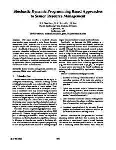
corner is at the position (W, H). To specify the position of an item i in the bin, we specify the coordinates of its bottom left corner. Using these conventions, it is not difficult to define more formally what is a pattern and how we can represent one. A guillotine pattern is a pattern that can be obtained by a sequence of guillotine cuts applied to the original bin and to the subsequent small rectangles that are obtained after each cut (see Figure 1). 1

2 7

3 4

5

6

Fig. 1. (a) Non-guillotine pattern; (b) Guillotine pattern.

3

The Problem GCV

In this section we focus on the Two-dimensional Guillotine Cutting Problem with Value (GCV). We present first some concepts and results needed to describe the algorithm. Let I = (W, H, w, h, v), with w = (w1 , . . . , wm ), h = (h1 , . . . , hm ) and v = (v1 , . . . , vm ), be an instance of the problem GCV. We consider that W , H, and the entries of w and h are all integer numbers. If this is not the case, we can obtain an equivalent integral instance simply by multiplying the widths and/or the heights of the bin and of the items by appropriate numbers. The first dynamic programming based algorithm for GCV was proposed by Gilmore and Gomory [18]. (It did not solve GCV in its general form.) We use here a dynamic programming approach for GCV that was proposed by Beasley [4] combined with the concept of discretization points defined by Herz [19]. A discretization point of the width (respectively of the height) is a value i ≤ W (respectively j ≤ H) that can be obtained by an integer conic combination of w1 , . . . , wm (respectively h1 , . . . , hm ). We denote by P (respectively Q) the set of all discretization points of the width (respectively height). Following Herz, we say a canonical pattern is a pattern for which all cuts are made at discretization points (e.g., the pattern indicated in Figure 1(b)). It is immediate that it suffices to consider only canonical patterns (for every pattern that is not canonical there is an equivalent one that is canonical). To refer to them, the following functions will be useful. For a rational x ≤ W , let p(x) := max (i | i ∈ P, i ≤ x) and for a rational y ≤ H, let q(y) := max (j | j ∈ Q, j ≤ y).

178


Using these functions, it is not difficult to verify that the recurrence formula below, proposed by Beasley [4], can be used to calculate the value V (w, h) of an optimal canonical guillotine pattern of a rectangle of dimensions (w, h). In this formula, v(w, h) denotes the value of the most valuable item that can be cut in a rectangle of dimensions (w, h), or 0 if no item can be cut in the rectangle. V (w, h) = max v(w, h), {V (w , h) + V (p(w − w ), h) | w ∈ P }, {V (w, h ) + V (w, q(h − h )) | h ∈ Q} .

(1)

Thus, if we calculate V (W, H) we have the value of an optimal solution for an instance I = (W, H, w, h, v). We can find the discretization points of the width (or height) by means of explicit enumeration, as we show in the algorithm DEE (Discretization by Explicit Enumeration) described below. In this algorithm, D represents the width (or height) of the bin and d1 , . . . , dm represent the widths (or heights) of the items. The algorithm DEE can be implemented to run in O(mδ) time, where δ represents the number of integer conic combinations of d1 , . . . , dm with value at most D. This means that when we multiply D, d1 , . . . , dm by a constant, the time required by DEE is not affected. √ It is easy to construct instances such that δ ≥ 2 D . Thus, an explicit enumeration may take exponential time. But if we can guarantee that di > D k (i = 1, . . . , m), the sum of the m coefficients of any integer conic combination of d1 , . . . , dm with value at most D is not greater than k. Thus, δ is at most the number of k-combinations of m objects with repetition. Therefore, for fixed k, δ is polynomial in m and consequently the algorithm DEE is polynomial in m. Algorithm 3.1 DEE Input: D (width or height), d1 , . . . , dm . Output: a set P of discretization points (of the width or height). P = ∅, k = 0. While k ≥ 0 do i−1 For i = k + 1mto m do zi = (D − j=1 dj zj )/di . P = P ∪ { j=1 zj dj }. k = max ({i | zi > 0, 1 ≤ i ≤ m} ∪ {−1}). If k > 0 then zk = zk − 1 and P = P ∪ { kj=1 zj dj }. Return P.

We can also use dynamic programming to find the discretization points. The basic idea is to solve a knapsack problem in which every item i has weight and value di (i = 1, . . . , m), and the knapsack has capacity D. The well-known dynamic programming technique for the knapsack problem (see [13]) gives the optimal value of knapsacks with (integer) capacities taking values from 1 to D.


179

It is easy to see that j is a discretization point if and only if the knapsack with capacity j has optimal value j. We have then an algorithm, which we call DDP (Discretization using Dynamical Programming), described in the sequel.

Algorithm 3.2 DDP Input: D, d1 , . . . , dm . Output: a set P of discretization points. P = {0}. For j = 0 to D do cj = 0. For i = 1 to m do For j = di to D If cj < cj−di + di then cj = cj−di + di For j = 1 to D If cj = j then P = P ∪ {j}. Return P.

We note that the algorithm DDP requires time O(mD). Thus, the scaling (if needed) to obtain an integral instance may render the use of DDP unsuitable in practice. On the other hand, the algorithm DDP is suited for instances in which D is small. If D is large but the dimensions of the items are not so small compared to the dimension of the bin, the algorithm DDP has a satisfactory performance. In the computational tests, presented in Section 5, we used the algorithm DDP. We describe now the algorithm DP that solves the recurrence formula (1). We have designed this algorithm in such a way that a pattern corresponding to an optimal solution can be easily obtained. For that, the algorithm stores in a matrix, for every rectangle of width w ∈ P and height h ∈ Q, which is the direction and the position of the first guillotine cut that has to be made in this rectangle. In case no cut should made in the rectangle, the algorithm stores which is the item that corresponds to this rectangle. When the algorithm DP halts, for each rectangle with dimensions (pi , qj ), we have that V (i, j) contains the optimal value that can be obtained in this rectangle, guillotine(i, j) indicates the direction of the first guillotine cut, and position(i, j) is the position (in the x-axis or in the y-axis) where the first guillotine cut has to be made. If guillotine(i, j) = nil, then no cut has to be made in this rectangle. In this case, item(i, j) (if nonzero) indicates which item corresponds to this rectangle. The value of the optimal solution will be in V (r, s). Note that each attribution of value to the variable t can be done in O(log r + log s) time by using binary search in the set of the discretization points. If we use the algorithm DEE to calculate the discretization points, the algorithm DP can be implemented to have time complexity O(δ1 + δ2 + r2 s log r + rs2 log s), where δ1 and δ2 represent the number of integer conic combinations that produce the discretization points of the width and of the height, respectively.

180


Algorithm 3.3 DP Input: An instance I = (W, H, w, h, v) of GCV, where w = (w1 , . . . , wm ), h = (h1 , . . . , hm ) and v = (v1 , . . . , vm ). Output: An optimal solution for I. Find p1 < . . . < pr , the discretization points of the width W . Find q1 < . . . < qs , the discretization points of the height H. For i = 1 to r For j = 1 to s V (i, j) = max ({vk | 1 ≤ k ≤ m, wk ≤ pi and hk ≤ qj } ∪ {0}). item(i, j) = max ({k | 1 ≤ k ≤ m, wk ≤ pi , hk ≤ qj and vk = V (i, j)} ∪ {0}). guillotine(i, j) = nil. For i = 2 to r For j = 2 to s n = max (k | 1 ≤ k ≤ r and pk ≤ p2i ). For x = 2 to n t = max (k | 1 ≤ k ≤ r and pk ≤ pi − px ). If V (i, j) < V (x, j) + V (t, j) then V (i, j) = V (x, j) + V (t, j), position(i, j) = px and guillotine(i, j) = ’V’. q n = max (k | 1 ≤ k ≤ s and qk ≤ 2j ). For y = 2 to n t = max (k | 1 ≤ k ≤ s and qk ≤ qj − qy ). If V (i, j) < V (i, y) + V (i, t) then V (i, j) = V (i, y) + V (i, t), position(i, j) = qy and guillotine(i, j) = ’H’.

H For the instances of GCV with wi > W k and hi > k (k fixed and i = 1, . . . , m), we have that δ1 , δ2 , r and s are polynomial in m. For such instances the algorithm DP requires time polynomial in m.

We can use a vector X (resp. Y ), of size W (resp. H), and let Xi (resp. Yj ) contain p(Xi ) (resp. q(Yj )). Once the discretization points are calculated, it requires time O(W + H) to determine the values in the vectors X and Y . Using these vectors, each attribution to the variable t can be done in constant time. In this case, an implementation of the algorithm DP, using DEE (resp. DDP) as a subroutine, would have time complexity O(δ1 + δ2 + W + H + r2 s + rs2 ) (resp. O(mW + mH + r2 s + rs2 )). In any case, the amount of memory required by the algorithm DP is O(rs). We can use the algorithm DP to solve the variant of GCV, denoted by GCVr , in which orthogonal rotations of the items are allowed. For that, given an instance I of GCVr , we construct another instance (for GCV) as follows. For each item i in I, of width wi , height hi and value vi , we add another item of width hi , height wi and value vi , whenever wi = hi , wi ≤ H and hi ≤ W .


4

181

The Problem GCD and the Column Generation Method

We focus now on the Two-dimensional Guillotine Cut Problem with Demands (GCD). First, let us formulate GCD as an ILP (Integer Linear Program). Let I = (W, H, w, h, d) be an instance of GCD. Represent each pattern j of the instance I as a vector pj , whose i-th entry indicates the number of times item i occurs in this pattern. The problem GCD consists then in deciding how many times each pattern has to be used to meet the demands and minimize the total number of bins that are used. Let n be the number of all possible patterns for I, and let P denote an m × n matrix whose columns are the patterns p1 , . . . , pn . If we denote by d the vector ofthe demands, then the following is an ILP n formulation for GCD: minimize j=1 xj subject to P x = d and xj ≥ 0 and xj integer for j = 1, . . . , n. (The variable xj indicates how many times the pattern j is selected.) Gilmore and Gomory [17] proposed a column generation method to solve the relaxation of the above ILP, shown below. The idea is to start with a few columns and then generate new columns of P , only when they are needed. minimize

x1 + . . . + xn

subject to P x = d xj ≥ 0

(2) j = 1, . . . , n.

The algorithm DP given in Section 3 finds guillotine patterns. Moreover, if each m item i has value yi and occurs zi times in a pattern produced by DP, then i=1 yi zi is maximum. This is exactly what we need to generate new columns. We describe below the algorithm SimplexCG2 that solves (2). The computational tests indicated that on the average the number of columns generated by SimplexCG2 was O(m2 ). This is in accordance with the theoretical results that are known with respect to the average behavior of the Simplex method [1,7]. We describe now a procedure to find an optimal integer solution from the solutions obtained by SimplexCG2 . The procedure is iterative. Each iteration starts with an instance I of GCD and consists basically in solving (2) with SimplexCG2 obtaining B and x. If x is integral, we return B and x and halt. Otherwise, we calculate x∗ = (x∗1 , . . . , x∗m ), where x∗i = xi (i = 1, . . . , m). For this new solution, possibly part of the demand of the items is not fulfilled. More the demand of each item i that is not fulfilled is d∗i = di − m precisely, ∗ ∗ ∗ ∗ j=1 Bi,j xj . Thus, if we take d = (d1 , . . . , dm ), we have a residual instance ∗ ∗ ∗ I = (W, H, l, c, d ) (we may eliminate from I the items with no demand). If some x∗i > 0 (i = 1, . . . , m), part of the demand is fulfilled by the solution ∗ x . In this case, we return B and x, we let I = I ∗ and start a new iteration. If x∗i = 0 (i = 1, . . . , m), no part of the demand is fulfilled by x∗ . We solve then the instance I ∗ with the algorithm Hybrid First Fit (HFF) [10]. We present in

182


Algorithm 4.1 SimplexCG2 Input: An instance I = (W, H, w, h, d) of GCD, where w = (w1 , . . . , wm ), h = (h1 , . . . , hm ) and d = (d1 , . . . , dm ). Output: An optimal solution for (2), where the columns of P are the patterns for I. 1 2 3 4 5 6

Let x = d and B be the identity matrix of order m. Solve y T B = 1IT . Generate a new column z executing the algorithm DP with parameters W, H, l, a, y. If y T z ≤ 1, return B and x and halt (x corresponds to the columns of B). Otherwise, solve Bw = z. x Let t = min( wjj | 1 ≤ j ≤ m, wj > 0). x

7 Let s = min(j | 1 ≤ j ≤ m, wjj = t). 8 For i = 1 to m do 8.1 Bi,s = zi . 8.2 If i = s then xi = t; otherwise, xi = xi − wi t. 9 Go to step 2.

what follows the algorithm CG that implements the iterative procedure we have described. Note that in each iteration either part of the demand is fulfilled or we go to step 4. Thus, after a finite number of iterations the demand will be met (part of it eventually in step 4). In fact, one can show that step 3.6 of the algorithm CG is executed at most m times. It should be noted however, that step 5 of the algorithm CG may require exponential time. This step is necessary to transform the representation of the last residual instance in an input for the algorithm HFF, called in the next step. Moreover, HFF may also take exponential time to solve this last instance. We designed an approximation algorithm for GCD, called SH, that makes use of the concept of semi-homogeneous patterns and has absolute performance bound 4 (see [12]). The reasons for not using SH, instead of HFF, to solve the last residual instance are the following: first, to generate a new column with the algorithm DP requires time that can be exponential in m. Thus, CG is already exponential, even on the average case. Besides that, the algorithm HFF has asymptotic approximation bound 2.125. Thus, we may expect that using HFF we may produce solutions of better quality. On the other hand, if the items are not too small with respect to the bin1 , the algorithm DP can be implemented to require polynomial time (as we mentioned in Section 3). In this case, we could eliminate steps 4 and 5 of CG and use SH instead of HFF to solve the last residual instance. The solutions may have worse quality, but at least, theoretically, the time required by such an algorithm would be polynomial in m, on the average. We note that the algorithm CG can be used to solve the variant of GCD, called GCDr , in which orthogonal rotations of the items are allowed. For that, 1

More precisely, for fixed k, wi >

W k

and hi >

H k

(i = 1, . . . , m).


183

Algorithm 4.2 CG Input: An instance I = (W, H, w, h, d) of GCD, where w = (w1 , . . . , wm ), h = (h1 , . . . , hm ) and d = (d1 , . . . , dm ). Output: A solution for I 1 Execute the algorithm SimplexCG2 with parameters W, H, l, a, d obtaining B and x. 2 For i = 1 to m do x∗i = xi . 3 If x∗i > 0 for some i, 1 ≤ i ≤ m, then 3.1 Return B and x∗1 , . . . , x∗m (but do not halt). 3.2 For i = 1 to m do 3.2.1 For j = 1 to m do di = di − Bi,j x∗j . 3.3 Let m = 0. 3.4 For i = 1 to m do 3.4.1 If di > 0 then m = m + 1, wm = wi , hm = hi and dm = di . 3.5 If m = 0 then halt. 3.6 Let m = m and go to step 1. 4 w = ∅, h = ∅. 5 For i = 1 to m do 5.1 For j = 1 to di do 5.1.1 w = w ∪ {wi }, h = h ∪ {hi }. 6 Return the solution of algorithm HFF executed with parameters W, H, w , h .

before we call the algorithm DP, in step 3 of SimplexCG2 , it suffices to make the transformation explained at the end of Section 3. We will call SimplexCGr2 the variant of SimplexCG2 with this transformation. It should be noted however that the algorithm HFF, called in step 6 of CG, does not use the fact that the items can be rotated. We designed a simple algorithm for the variant of GCDr in which all items have demand 1, called here GCDBr . This algorithm, called First Fit Decreasing Height using Rotations (FFDHR), has asymptotic approximation bound at most 4, as we have shown in [12]. Substituting the call to HFF with a call to FFDHR, we obtain the algorithm CGR, that is a specialized version of CG for the problem GCDr . We also tested another modification of the algorithm CG (and of CGR). This is the following: when we solve an instance, and the solution returned by SimplexCG2 rounded down is equal to zero, instead of submitting this instance to HFF (or FFDHR), we use HFF (or FFDHR) to obtain a good pattern, updating the demands, and if there is some item for which the demand is not fulfilled, we go to step 1. Note that, the basic idea is to perturb the residual instances whose relaxed LP solution, rounded down, is equal to zero. With this procedure, it is expected that the solution obtained by SimplexCG2 for the residual instance has more variables with value greater than 1. The algorithm CG p , described below, incorporates this modification. It should be noted that with this modification we cannot guarantee anymore that we have to make at most m + 1 calls to SimplexCG2 . It is however, easy

184


Algorithm 4.3 GC p Input: An instance I = (W, H, w, h, d) of GCD, where w = (w1 , . . . , wm ), h = (h1 , . . . , hm ) and d = (d1 , . . . , dm ). Output: A solution for I 1 Execute the algorithm SimplexCG2 with parameters W, H, w, h, d obtaining B and x. 2 For i = 1 to m do x∗i = xi . 3 If x∗i > 0 for some i, 1 ≤ i ≤ m, then 3.1 Return B and x∗1 , . . . , x∗m (but do not halt). 3.2 For i = 1 to m do 3.2.1 For j = 1 to m do di = di − Bi,j x∗j . 3.3 Let m = 0. 3.4 For i = 1 to m do 3.4.1 If di > 0 then m = m + 1, wm = wi , hm = hi and dm = di . 3.5 If m = 0 then halt. 3.6 Let m = m and go to step 1. 4 w = ∅, h = ∅. 5 For i = 1 to m do 5.1 For j = 1 to di do 5.1.1 w = w ∪ {wi }, h = h ∪ {hi }. 6 Return a pattern generated by the algorithm HFF, executed with parameters W, H, w , h , that has the smallest waste of area, and update the demands. 7 If there are demands to be fulfilled, go to step 1.

to see that the algorithm CG p in fact halts, as each time step 1 is executed, the demand decreases strictly. After a finite number of iterations the demand will be fulfilled and the algorithm halts (in step 3.5 or step 7).

5

Computational Results

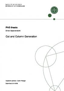
The algorithms described in sections 3 and 4 were implemented in C language, using Xpress-MP [27] as the LP solver. The tests were run on a computer with two processors AMD Athlon MP 1800+, clock of 1.5 Ghz, memory of 3.5 GB and operating system Linux (distribution Debian GNU/Linux 3.0 ). The performance of the algorithm DP was tested with the instances of GCV available in the OR-LIBRARY2 (see Beasley [6] for a brief description of this library). We considered the 13 instances of GCV, called gcut1, . . . , gcut13 available in this library. For all these instances, with exception of instance gcut13, optimal solutions had already been found [4]. We solved to optimality this instance as well. In these instances the bins are squares, with dimensions between 250 and 3000, and number of items (m) between 10 and 50. The value of each item is precisely its area. We show in Figure 2 the optimal solution for gcut13 found by the algorithm DP. 2

http://mscmga.ms.ic.ac.uk/info.html


185

200x378 200x378 200x378 200x378 200x378 200x378 200x378 200x378 200x378 200x378 200x378 200x378 200x378 200x378 200x378





496x555

496x555

496x555

755x555

755x555

496x555

496x555

496x555

755x555

755x555

Fig. 2. The optimal solution for gcut13 found by the algorithm DP.

In Table 1 we show the characteristics of the instances solved and the computational results. The column “Waste” gives —for each solution found— the percentage of the area of the bin that does not correspond to any item. Each instance was solved 100 times; the column “Time” shows the average CPU time in seconds, considering all these 100 resolutions. We have also tested the algorithm DP for the instances gcut1, . . . , gcut13, this time allowing rotations (we called these instances gcut1r, . . . , gcut13r). Owing to space limitations, we omit the table showing the computational results. It can be found at http://www.ime.usp.br/$\sim$glauber/gcut. We only remark that for some instances the time increased (it did not doubled) but the waste decreased, as one would expect. We did not find instances for GCD in the OR-LIBRARY. We have then tested the algorithms CG and CG p with the instances gcut1, . . . , gcut12, associating with each item i a randomly generated demand di between 1 and 100. We called these instances gcut1d, . . . , gcut12d. We show in Table 2 the computational results obtained with the algorithm CG. In this table, LB denotes the lower bound (given by the solution of (2)) for the value of an optimal integer solution. Each instance was solved 10 times; the column “Average Time” shows the average time considering these 10 experiments. The algorithm CG found optimal or quasi-optimal solutions for all these instances. On the average, the difference between the solution found by CG and the lower bound (LB) was only 0,161%. We note also that the time spent to solve these instances was satisfactory. Moreover, the gain of the solution of CG

186

G. Cintra and Y. Wakabayashi Table 1. Performance of the algorithm DP. Quantity Instance of items gcut1 10 gcut2 20 gcut3 30 gcut4 50 gcut5 10 gcut6 20 gcut7 30 gcut8 50 gcut9 10 gcut10 20 gcut11 30 gcut12 50 gcut13 32

Dimensions of the bin (250, 250) (250, 250) (250, 250) (250, 250) (500, 500) (500, 500) (500, 500) (500, 500) (1000, 1000) (1000, 1000) (1000, 1000) (1000, 1000) (3000, 3000)

r 19 112 107 146 76 120 126 262 41 155 326 363 2425

s 68 95 143 146 39 95 179 225 91 89 238 398 1891

Optimal Solution 56460 60536 61036 61698 246000 238998 242567 246633 971100 982025 980096 979986 8997780

Waste 9,664% 3,142% 2,342% 1,283% 1,600% 4,401% 2,973% 1,347% 2,890% 1,798% 1,990% 2,001% 0,025%

Time (sec) 0,003 0,010 0,012 0,022 0,004 0,008 0,017 0,062 0,006 0,009 0,066 0,140 144,915

compared to the solution of HFF was 8,779%, on the average, a very significant improvement. We have also used the algorithm CG p to solve the instances gcut1d, . . . , gcut12d. The results are shown in Table 3. We note that the number of columns generated increased approximately 40%, on the average, and the time spent increased approximately 15%, on the average. On the other hand, an optimal solution was found for the instance gcut4d. We also considered the instances gcut1d, . . . , gcut12d as being for the problem GCDr (rotations are allowed), and called them gcut1dr, . . . , gcut12dr. We omit the table with the computational results we have obtained (the reader can find it at the URL we mentioned before). We only remark that the algorithm CGR found optimal or quasi-optimal solutions for all instances. The difference between the value found by CGR and the lower bound (LB) was only 0,408%, on the average. Comparing the value of the solutions obtained by CGR with the solutions obtained by FFDHR, we note that there was an improvement of 12,147%, on the average. This improvement would be of 16,168% if compared with the solution obtained by HFF. The instances gcut1dr, . . . , gcut12dr were also tested with the algorithm CGRp . The computational results are shown in Table 4. We remark that the performance of the algorithm CGRp was a little better than the performance of CGR, with respect to the quality of the solutions. The difference between the value of the solution obtained by CGRp and the lower bound decreased to 0,237%, on the average. The gain on the quality was obtained at the cost of an increase of approximately 97% (on the average) of the number of columns generated and of an increase of approximately 44% of time.


187

Table 2. Performance of the algorithm CG. Solution Instance of CG gcut1d 294 gcut2d 345 gcut3d 333 gcut4d 838 gcut5d 198 gcut6d 344 gcut7d 591 gcut8d 691 gcut9d 131 gcut10d 293 gcut11d 331 gcut12d 673

6

LB 294 345 332 836 197 343 591 690 131 293 330 672

Difference Average Columns Solution Improvement from LB Time (sec) Generated of HFF over HFF 0,000% 0,059 9 295 0,339% 0,000% 0,585 68 402 14,179% 0,301% 2,340 274 393 14,834% 0,239% 11,693 820 977 11,323% 0,507% 0,088 18 198 0,000% 0,291% 0,362 101 418 17,308% 0,000% 1,184 136 615 4,523% 0,145% 30,361 952 764 9,555% 0,000% 0,068 11 143 7,092% 0,000% 0,172 20 335 12,537% 0,303% 8,570 222 353 6,232% 0,149% 39,032 485 727 7,428%

Concluding Remarks

In this paper we presented algorithms for the problems GCV and GCD and their variants GCVr and GCDr . For the problem GCV we presented the (exact) pseudo-polynomial algorithm DP. This algorithm can either use the algorithm DDE or DDP to generate the discretization points. Both of these algorithms were described. We have also shown that these algorithms can be implemented to run in polynomial time when the items are not so small compared to the size of the bin. In this case the algorithm DP also runs in polynomial time. We have also mentioned how to use DP to solve the problem GCVr . We presented two column generation based algorithms to solve GCD: CG and CG p . Both use the algorithm DP to generate the columns: the first uses the algorithm HFF to solve the last residual instance and the second uses a perturbation strategy. The algorithm CG combines different techniques: Simplex method with column generation, an exact algorithm for the discretization points, and an approximation algorithm (HFF) for the last residual instance. An approach of this nature has shown to be promising, and has been used in the one-dimensional cutting problem with demands [26,11]. The algorithm CG p is a variant of CG, in which we use an idea that consists in perturbing the residual instances. We have also designed the algorithms CGR and CGRp , for the problem GCDr , a variation of GCD in which orthogonal rotations are allowed. The algorithm CGR uses as a subroutine the algorithm FFDHR, we have designed. We noted that the algorithm CG and CGR are polynomial, on the average, when the items are not so small compared to the size of the bin. The computational results with these algorithms were very satisfactory: optimal or quasioptimal solutions were found for the instances we have considered. As expected,

188

G. Cintra and Y. Wakabayashi Table 3. Performance of the algorithm CG p .

Solution Instance of CG p gcut1d 294 gcut2d 345 gcut3d 333 gcut4d 837 gcut5d 198 gcut6d 344 gcut7d 591 gcut8d 691 gcut9d 131 gcut10d 293 gcut11d 331 gcut12d 673

LB 294 345 332 836 197 343 591 690 131 293 330 672

Difference Average Columns Solution Improvement from LB Time (sec) Generated of HFF over HFF 0,000% 0,034 9 295 0,339% 0,000% 0,552 68 402 14,179% 0,301% 3,814 492 393 14,834% 0,120% 16,691 1271 977 11,429% 0,507% 0,086 25 198 0,000% 0,291% 0,400 121 418 17,308% 0,000% 1,202 136 615 4,523% 0,145% 32,757 1106 764 9,555% 0,000% 0,042 11 143 7,092% 0,000% 0,153 20 335 12,537% 0,303% 10,875 416 353 6,232% 0,149% 42,616 692 727 7,428%

CG p (respectively CGRp ) found solutions of a little better quality than CG (respectively CGR) at the cost of a slight increase in the running time. We exhibit in Table 5 the list of the algorithms we proposed in this paper. A natural development of our work would be to adapt the approach used in the algorithm CG to the Two-dimensional cutting stock problem with demands (CSD), a variant of GCD in which the cuts need not be guillotine. One can find an initial solution using homogeneous patterns; the columns can be generated using any of the algorithms that have appeared in the literature for the twodimensional cutting stock problem with value [5,2]. To solve the last residual instance one can use approximation algorithms [10,8,20]. One can also use column generation for the variant of CSD in which the quantity of items in each bin is bounded. This variant, proposed by Christofides and Whitlock [9], is called restricted two-dimensional cutting stock problem. Each new column can be generated with any of the known algorithms for the restricted two-dimensional cutting stock problem with value [9,24], and the last residual instance can be solved with the algorithm HFF. This restricted version with guillotine cut requirement can also be solved using the ideas we have just described: the homogeneous patterns and the patterns produced by HFF can be obtained with guillotine cuts, and the columns can be generated with the algorithm of Cung, Hifi and Le Cun [16]. A more audacious step would be to adapt the column generation approach for the three-dimensional cutting stock problem with demands. For the initial solutions one can use homogeneous patterns. The last residual instances can be dealt with some approximation algorithms for the three-dimensional bin packing problem [3,14,15,22,23,21,25]. We do no know however, exact algorithms to generate columns. If we require the cuts to be guillotine, one can adapt the algorithm DP to generate new columns.


189

Table 4. Performance of the algorithm CGRp . Solution Instance of CGRp gcut1dr 291 gcut2dr 283 gcut3dr 314 gcut4dr 837 gcut5dr 175 gcut6dr 301 gcut7dr 542 gcut8dr 651 gcut9dr 123 gcut10dr 270 gcut11dr 299 gcut12dr 602

LB 291 282 313 836 174 301 542 650 122 270 298 601

Difference Average Columns Solution Improvement from LB Time (sec) Generated of FFDHR over FFDHR 0,000% 0,070 5 291 0,000% 0,355% 5,041 252 330 14,242% 0,319% 10,006 740 355 11,549% 0,120% 25,042 1232 945 11,429% 0,575% 0,537 58 200 12,500% 0,000% 2,884 175 405 25,679% 0,000% 4,098 121 599 9,516% 0,153% 68,410 1154 735 11,429% 0,820% 0,494 42 140 12,143% 0,000% 1,546 33 330 18,182% 0,336% 86,285 686 329 9,119% 0,166% 181,056 945 682 11,730%

Table 5. Algorithms proposed in this paper. Algorithm DP DEE DDP CG CG p CGR CGRp

Problems GCV and GCVr Discretization points Discretization points GCD GCD GCDr GCDr

Comments Polynomial for large items Polynomial for large items Polynomial, on the average, for large items Polynomial, on the average, for large items

References 1. Ilan Adler, Nimrod Megiddo, and Michael J. Todd. New results on the average behavior of simplex algorithms. Bull. Amer. Math. Soc. (N.S.), 11(2):378–382, 1984. 2. M. Arenales and R. Mor´ abito. An and/or-graph approach to the solution of twodimensional non-guillotine cutting problems. European Journal of Operations Research, 84:599–617, 1995. 3. N. Bansal and M. Srividenko. New approximability and inapproximability results for 2-dimensional bin packing. In Proceedings of 15th ACM-SIAM Symposium on Discrete Algorithms, pages 189–196, New York, 2004. ACM. 4. J. E. Beasley. Algorithms for unconstrained two-dimensional guillotine cutting. Journal of the Operational Research Society, 36(4):297–306, 1985. 5. J. E. Beasley. An exact two-dimensional nonguillotine cutting tree search procedure. Oper. Res., 33(1):49–64, 1985. 6. J. E. Beasley. Or-library: distributing test problems by electronic mail. Journal of the Operational Research Society, 41(11):1069–1072, 1990. 7. Karl-Heinz Borgwardt. Probabilistic analysis of the simplex method. In Mathematical developments arising from linear programming (Brunswick, ME, 1988), volume 114 of Contemp. Math., pages 21–34. Amer. Math. Soc., Providence, RI, 1990.

190


8. A. Caprara. Packing 2-dimensional bins in harmony. In Proceedings of the 43-rd Annual IEEE Symposium on Foundations of Computer Science, pages 490–499. IEEE Computer Society, 2002. 9. N. Christofides and C. Whitlock. An algorithm for two dimensional cutting problems. Operations Research, 25:30–44, 1977. 10. F. R. K. Chung, M. R. Garey, and D. S. Johnson. On packing two-dimensional bins. SIAM J. Algebraic Discrete Methods, 3:66–76, 1982. 11. G. F. Cintra. Algoritmos h´ıbridos para o problema de corte unidimensional. In XXV Conferência Latinoamericana de Inform´ atica, Assun¸ca õ, 1999. 12. G. F. Cintra. Algoritmos para problemas de corte de guilhotina bidimensional (PhD thesis in preparation). Instituto de Matem´ atica e Estat´ıstica, 2004. 13. Thomas H. Cormen, Charles E. Leiserson, Ronald L. Rivest, and Clifford Stein. Introduction to algorithms. MIT Press, Cambridge, MA, second edition, 2001. 14. J.R. Correa and C. Kenyon. Approximation schemes for multidimensional packing. In Proceedings of 15th ACM-SIAM Symposium on Discrete Algorithms, pages 179– 188, New York, 2004. ACM. 15. J. Csirik and A. Van Vliet. An on-line algorithm for multidimensional bin packing. Operations Research Letters, 13:149–158, 1993. 16. Van-Dat Cung, Mhand Hifi, and Bertrand Le Cun. Constrained two-dimensional cutting stock problems a best-first branch-and-bound algorithm. Int. Trans. Oper. Res., 7(3):185–210, 2000. 17. P. Gilmore and R. Gomory. A linear programming approach to the cutting stock problem. Operations Research, 9:849–859, 1961. 18. P. Gilmore and R. Gomory. Multistage cutting stock problems of two and more dimensions. Operations Research, 13:94–120, 1965. 19. J. C. Herz. A recursive computational procedure for two-dimensional stock-cutting. IBM Journal of Research Development, pages 462–469, 1972. 20. Claire Kenyon and Eric Rémila. A near-optimal solution to a two-dimensional cutting stock problem. Math. Oper. Res., 25(4):645–656, 2000. 21. Y. Kohayakawa, F.K. Miyazawa, P. Raghavan, and Y. Wakabayashi. Multidimensional cube packing. In Brazilian Symposium on Graphs and Combinatorics. Electronic Notes of Discrete Mathematics (GRACO’2001). Elsevier Science, 2001. (to appear in Algorithmica). 22. Keqin Li and Kam-Hoi Cheng. Generalized first-fit algorithms in two and three dimensions. Internat. J. Found. Comput. Sci., 1(2):131–150, 1990. 23. F. K. Miyazawa and Y. Wakabayashi. Parametric on-line algorithms for packing rectangles and boxes. European J. Oper. Res., 150(2):281–292, 2003. 24. J. F. Oliveira and J. S. Ferreira. An improved version of Wang’s algorithm for twodimensional cutting problems. European Journal of Operations Research, 44:256– 266, 1990. 25. S. Seiden and R. van Stee. New bounds for multidimensional packing. Algorithmica, 36:261–293, 2003. 26. G. W¨ ascher and T. Gau. Heuristics for the integer one-dimensional cutting stock problem: a computational study. OR Spektrum, 18:131–144, 1996. 27. Xpress. Xpress Optimizer Reference Manual. DASH Optimization, Inc, 2002.