Dynamic Programming Guided Exploration for Sampling-based Motion Planning Algorithms Oktay Arslan1
Abstract— Several sampling-based algorithms have been recently proposed that ensure asymptotic optimality. The convergence of these algorithms can be improved if sampling is guided toward the most promising region of the search space where the solution is more likely to be found. In this paper we propose three sample rejection methods that leverage the classification of the samples according to their potential of being part of the optimal solution to guide the exploration of the motion planner to promising regions of the search space. These sampling strategies are a direct by-product of the exploitation phase of the algorithm, which uses a dynamic programming (DP) step while planning on random graphs as, for example, is done in the RRT# algorithm. It is shown that the proposed sampling strategies are able to compute high-quality solutions, much faster than existing algorithms. We provide numerical results and compare the performance of the proposed algorithm with the original RRT# and the RRT∗ algorithms.
I. I NTRODUCTION A bottleneck in most motion planning problems, especially those involving systems with high state dimensionality, is the computational overhead associated with discretizing the state space. Hence deterministic searches are impractical for high dimensional search spaces. Probabilistic methods, on the other hand, have proven to be very efficient for the solution of motion planning problems with dynamic constraints in high dimensional search spaces. Among them, incremental sampling-based motion planning algorithms, such as the Rapidly-exploring Random Trees (RRT) [21], and the Probabilistic Road Maps (PRM) [8], [15], [16], [6, Ch. 7] have become very popular, owing to their implementation simplicity and their advantages in handling high-dimensional problems. Moreover, these algorithms have been recently applied to many other interesting applications including pursuit-evasion games, stochastic optimal motion planning problems [13], [12], [2]. Although these algorithms work very well in practice, the solution may be far from the optimal one. Recent algorithms, notably the RRT∗ and the PRM∗ algorithms, bypass this drawback and ensure asymptotic optimality as the number of samples tends to infinity. Nonetheless, the convergence rate to the optimal solution of the RRT∗ and PRM∗ algorithms may still be slow, as demonstrated by several motion planning problems of robotic manipulation. One of the main reasons of the slow convergence of asymptotically optimal algorithms is the lack of a good ex1 Oktay Arslan is a Robotics, PhD Candidate with the D. Guggenheim School of Aerospace Engineering and the Institute for Robotics and Intelligent Machines at the Georgia Institute of Technology, Atlanta, GA 303320150, USA, Email:
[email protected] 2 Panagiotis Tsiotras is with the faculty of D. Guggenheim School of Aerospace Engineering and the Institute for Robotics and Intelligent Machines at the Georgia Institute of Technology, Atlanta, GA 30332-0150, USA, Email:
[email protected]
Panagiotis Tsiotras2
ploration strategy. Most current planners use an exploration strategy whose only goal is to gather samples from the free space. Although every collected sample gives some information about the topology of the search space, it may not necessarily contribute to improving the cost of the solution of a given query. Since the exploration task (e.g., sampling, collision checking) is one of main computational bottlenecks of sampling-based motion planners, it is preferable to select samples that maximize the improvement of the quality of the solution of a given query (i.e., contribute most to the exploitation step). One way to achieve this is to guide exploration to the region of the search space that is relevant to the current query, i.e., the subset of the search space in which the optimal solution lies. The concept of “relevant” region is not new and has been essential in the success and the wide applicability of the A∗ algorithm [11]. As it is well known, with the help of an admissible heuristic, the A∗ algorithm expands a much smaller number of vertices than that of Dijkstra’s algorithm [7]. This set of expanded vertices corresponds to the “relevant” region of the query of interest, that is, these vertices have the potential to be part of the optimal solution. Note that if the heuristic used is the exact “cost-to-go” for each vertex, the relevant region would consist only of the vertices of the optimal solution. The same approach can be incorporated to sampling-based motion planners by approximating the relevant region of a query and adjusting the sampling strategy to draw more samples from the relevant region. Computing the relevant region is not easy, of course, but recently a new samplingbased motion planning algorithm, called RRT# , has been proposed which computes successively tighter approximations of the relevant region of the search space as the number of samples tend to infinity as a by-product of the exploitation step [3]. Specifically, and similarly to the RRT∗ algorithm, the RRT# algorithm utilizes ideas from Rapidly-exploring Random Graphs (RRG) but, in addition, it also incorporates a relaxation step, as used in dynamic programming [4], [5], in order to solve the optimal motion planning problem more efficiently. As shown in [3] the RRT# algorithm has a faster convergence rate and provides solutions with smaller variance compared to the RRT∗ algorithm. The RRT# algorithm also provides a good characterization of the computed information during the search, by identifying the region of the search space which is highly likely to contain the optimal solution. It is then natural to leverage this property of the RRT# algorithm to guide the selection of future samples to improve the overall convergence properties of the algorithm. This is precisely the main contribution of this paper. By interleaving the exploitation and exploration steps of the RRT# algorithm, we show significant improvements
in terms of the convergence rate of asymptotically optimal sampling-based algorithms using a number of non-trivial path-planning scenarios. In this paper we develop three extensions of the baseline RRT# algorithm, originally proposed in [3], which use certain sample rejection criteria in order to reduce the number of vertices that are sampled (and eventually added to the search graph). As a result, the possibility of including samples in the unfavorable region of the search space is greatly reduced. We give a detailed explanation of this sample rejection method via extensive numerical simulations. For demonstration purposes, we first test the proposed algorithm on simple problems in 2D where the effect of sample rejection method is evident and is easily visualized. Then, we consider a pathological case in which the heuristic is less informative than that of in former environments. We finally apply the proposed algorithms to two more challenging path-planning problems in high dimensional search spaces, namely, a single-arm (6 DoFs) and a dual-arms (12 DoFs) manipulation task for a humanoid robot. We benchmark the performance of all these algorithms against the RRT∗ and the baseline RRT# algorithms. Our numerical simulations demonstrate that these new extensions of RRT# reduce the number vertices in the graph significantly, yet they are all able to compute high quality paths in much shorter time. II. P ROBLEM F ORMULATION A. Notation and Definitions Let X denote the configuration space, which is an open subset of Rd , where d is a positive integer such that d ≥ 2. Let the obstacle region and the goal region be denoted by Xobs and Xgoal , respectively. The obstacle-free space is defined by Xfree = X \ Xobs . Let the initial configuration be denoted by xinit ∈ Xfree . We will use graphs to represent the connections between a (finite) set of configuration points selected randomly from Xfree . Let G = (V, E) denote such a graph, where V and E ⊆ V × V are finite sets of vertices and edges, respectively. Given a vertex v ∈ V in a directed graph G = (V, E), succ(G, v) returns the vertices in V that can be reached from vertex v, pred(G, v) returns the vertices in V that are the tails of the edges going into v, parent(v) returns a unique vertex u ∈ V such that (u, v) ∈ E and u ∈ pred(G, v) and a spanning tree of G can be defined such that T = (Vs , Es ), where Vs = V , Es = {(u, v) : (u, v) ∈ E and parent(v) = u}. Given an edge e = (u, v) ∈ E, the function c : e 7→ r returns a non-negative real number so that c(u, v), where v ∈ succ(G, u), is the cost incurred by moving from u to v. In this work it is assumed that transition costs are symmetric, that is, c(x, x0 ) = c(x0 , x). The function g : v 7→ r returns a non-negative real number r, which is the cost of the path to v from a given initial state xinit ∈ Xfree . The function lmc : v 7→ r returns a non-negative real number r, which is the one-step lookahead cost-to come estimate of the vertex v, called the locally minimum cost-to-come estimate, or lmc-value of the vertex for short (see [3], also called rhs-value in [19]). We will use g∗ (v) to denote the optimal cost-to-come value of the vertex v which can be achieved in Xfree . Given a goal region Xgoal , the function h : (v, Xgoal ) 7→ r returns an estimate r of the optimal cost from v to Xgoal ; we set h(v) = 0 if v ∈ Xgoal .
B. Problem Statement We wish to solve the following motion planning problem: Given a bounded and connected open set X ⊂ Rd , the sets Xfree and Xobs = X \Xfree , and an initial point xinit ∈ Xfree and a goal region Xgoal ⊂ Xfree , find the minimum-cost path connecting xinit to the goal region Xgoal . III. M OTION P LANNING A LGORITHMS A. The RRT# Algorithm In order to understand how the proposed algorithms work, we first have to revisit the baseline RRT# algorithm from [3] and understand how RRT# makes decisions which vertex to explore next, based on a relaxation step. Note that the latter step is similar to what it is implemented in the LPA∗ algorithm [19], [17], [18]. The RRT# algorithm performs two tasks, namely exploration and exploitation, during each iteration. The exploration task implements the extension procedure of the RRG algorithm, and this task is subsequently followed by an exploitation step that implements the GaussSeidel version of the Bellman-Ford algorithm. Algorithm 1: Body of the RRT# Algorithm 1 2 3 4 5 6 7
RRT# (xinit , Xgoal , X ) V ← {xinit }; E ← ∅; G ← (V , E); for k = 1 to N do xrand ← Sample(k); G ← Extend(G, xrand ); Replan(G, Xgoal );
10
(V , E) ← G; E 0 ← ∅; foreach x ∈ V do E 0 ← E 0 ∪ {(parent(x), x)};
11
return T = (V , E 0 );
8 9
A brief description of the main procedures used by the RRT# algorithm in [3] is given below. The following procedures are inherited from the RRT∗ algorithm [14]. Sample : N → Xfree returns independent, identically distributed samples from Xfree . Nearest returns a point from a given finite set V , which is the closest to a given point x in terms of a given distance function. Near returns a collection of points, from a given finite set V , within the closed ballnof radius rn centered atoa given point x , where 1/d rn = min ((γ log n)/(ζd n)) , η , η is steering radius, γ is a constant, ζd is the volume of unit ball in d-dimensional space. Steer returns the point in a ball centered around a given state x that is closest, with respect to the given distance function, to another given point xnew . Given two points x1 , x2 ∈ Xfree , the Boolean function ObstacleFree(x1 , x2 ) checks whether the line segment connecting these two points belongs to Xfree . It returns True if the line segment is a subset of Xfree . Extend is a function that extends the nearest vertex of the graph G toward the randomly sampled point xrand . In addition, our proposed algorithms use the following procedures. Ordering: Given a vertex v ∈ V , the function Key : v 7→ k returns a real vector k ∈ R2 , whose components are k1 (v) = lmc(v) + h(v) and k2 (v) = lmc(v). Given two keys k1 , k2 ∈ R2 , the Boolean function 4 : (k1 , k2 ) 7→
Algorithm 2: Replan Procedure# 1 2 3 4 5 6 7 8 9 10
Algorithm 3: Auxiliary Procedures#
Replan(G,Xgoal ) ∗ while q.f indmin() ≺ Key(vgoal ) do x = q.f indmin(); g(x) = lmc(x); q.delete(x); foreach s ∈ succ(G, x) do if lmc(s) > g(x) + c(x, s) then lmc(s) = g(x) + c(x, s); parent(s) = x; UpdateQueue(s);
1 2 3 4 5 6 7 8 9 10 11 12 13
{False, True} returns True if and only if either k11 < k21 or (k11 = k21 and k12 ≤ k22 ), and returns False otherwise. Promising vertices: Given a graph G = (V, E) with xinit ∈ V , let g∗ (v) be the optimal cost-to-come value of the vertex v that can be achieved on the given graph G, and ∗ let vgoal = argminv∈V ∩Xgoal g∗ (v). The set of promising vertices Vprom ⊂ V is defined by Vprom = {v : [f(v), g∗ (v)] ≺ ∗ ∗ [f(vgoal ), g∗ (vgoal )]}, where f(v) = g∗ (v) + h(v). Only promising vertices have the potential to be part of the optimal path from xinit to Xgoal . Therefore, all promising vertices must be stationary at the end of each iteration. Relevant region: Let x∗goal ∈ Xgoal be the point in the goal region that has the lowest optimal cost-to-come value in Xgoal , i.e., x∗goal = argminx∈Xgoal g∗ (x). The relevant region of Xfree is the set of points x for which the optimal cost-tocome value of x, plus the estimate of the optimal cost moving from x to Xgoal is less than the optimal cost-to-come value of x∗goal , that is, Xrel = {x ∈ Xfree : g∗ (x) + h(x) < g∗ (x∗goal )}.
(1)
Points of Xrel have the potential to be part of the optimal path starting at xinit and reaching Xgoal . Replanning: Given a graph G k = (V k , E k ) at the kth iteration, a goal region Xgoal ⊂ Xfree and an arbitrary vector g k−1,0 ∈ Rnk of cost-to-come values of all v ∈ V k , where gik−1,0 = 0 for vi = xinit , the function Replan : (G k , Xgoal , g k−1,0 ) 7→ (G k , Xgoal , g k,0 ) operates on the nonstationary vertices iteratively until all promising vertices become stationary. Priority of vertices: The priority of vertices is the same as the priority of their associated keys, and a priority queue is used to sort all of the nonstationary vertices of the graph based on their respective key values. The function UpdateQueue changes the queue based on the g- and lmcvalues of the vertex v. If the vertex v is nonstationary, then it is either inserted into the queue or its priority in the queue is updated based on its up-to-date key value if it is already inside the queue. Otherwise, the vertex is removed from the queue if it is a stationary vertex. The order of expanded vertices is determined by selecting the vertex of minimum key value in the queue for expansion at each step. The main body of the RRT# algorithm is given in Algorithm 1. The algorithm starts by adding the initial point xinit into the vertex set of the underlying graph. Then, it incrementally grows the graph in Xfree by sampling randomly a point xrand from Xfree and extending the graph toward
14 15
Initialize(x, x0 ) g(x) ← ∞; lmc(x) ← ∞; parent(x) ← x0 ; if x0 6= ∅ then lmc(x) ← g(x0 ) + c(x0 , x); UpdateQueue(x) if g(x) 6= lmc(x) and x ∈ q then q.update(x, Key(x)); else if g(x) 6= lmc(x) and x ∈ / q then q.insert(x, Key(x)); else if g(x) = lmc(x) and x ∈ q then q.delete(x); Key(s) return k = (lmc(x) + h(x), lmc(x));
Algorithm 4: Extend Procedure#
13
Extend(G,x) (V , E) ← G; E 0 ← ∅; xnearest ← Nearest(G, x); xnew ← Steer(xnearest , x); if ObstacleFree(xnearest , xnew ) then Initialize(xnew , ∅); Xnear ← Near(G, xnew , |V |); foreach xnear ∈ Xnear do if ObstacleFree(xnear , xnew ) then lmc0 (xnew ) = g(xnear ) + c(xnear , xnew ); if lmc(xnew ) > lmc0 (xnew ) then lmc(xnew ) = lmc0 (xnew ); parent(xnew ) = xnear ;
14
E 0 ← E 0 ∪ {(xnear , xnew ), (xnew , xnear )};
1 2 3 4 5 6 7 8 9 10 11 12
15 16 17 18 19
if IncludeVertex(xnew ) then V ← V ∪ {xnew }; E ← E ∪ E0; UpdateQueue(xnew ); return G 0 ← (V , E);
xrand . In this paper we utilize adaptive rejection sampling into the extension step of the RRT# algorithm, and propose a new Extend procedure, which is given in Algorithm 4. The Replan procedure, which is provided in Algorithm 2, then propagates the new information due to the extension across the whole graph in order to improve the cost-to-come values of the promising vertices in the graph. This process is repeated for a given fixed number of iterations. The spanning tree of the final graph which is rooted at the initial vertex, and which contains the lowest-cost path information for the ∗ promising vertices and vgoal , is returned at the end. IV. P ROPOSED S AMPLING S TRATEGIES A. Adaptive Sampling Strategies Along with planning algorithms, sampling methods are crucial components of randomized motion planners and have a huge impact on the overall performance of the search process. Since randomized motion planners are not provided the search space explicitly a priori, they may perform poorly,
or even fail to find a solution, if the sampling method used is not capable of generating a good number of high quality samples for a fixed number of iterations. Properties of high quality samples (at least na¨ıvely) can be stated as: first being collision-free, and second yielding a significant improvement on the quality of the path computed thus far. This is owing to the fact that asymptotically optimal motion planners aim to find the lowest-cost path as the number of iterations goes to infinity. Achieving these two properties for randomly drawn samples makes the sampling process a challenging task, essentially implying that the samples should be drawn from a (unknown) nonuniform probability density function defined over the whole configuration space, a difficult task in general. Several heuristics have been proposed in the past and integrated to sampling-based motion planners to help efficient exploration. The main idea of these approaches is to efficiently evaluate the potential of a sample to be part of the optimal solution in a given query. Note that one can give a characterization of all samples that form the optimal solution using the equality c∗ (xinit , x) + c∗ (x, xgoal ) = c∗ (xinit , xgoal ), where c∗ (x, x0 ) denotes the optimal cost connecting points x and x0 . Since the optimal cost of these connections are not known in a priori, the previous condition is relaxed, and a heuristic is used, instead, to evaluate the cost of a potential path starting from xinit to xgoal and passing through x. Therefore, the main challenge in developing good sampling strategies is to compute efficiently a highly accurate estimate of the optimal connection costs between xinit , x and xgoal . Given such an admissible heuristic h, a sampling strategy can be developed by rejecting samples outside the hyper-ellipse defined by h(xinit , x) + h(x, xgoal ) < cbest (xinit , xgoal ), where cbest is the cost of the current best path computed by the algorithm [9], [22]. Although this sampling strategy is the easiest to implement, it will add many useless samples if the heuristic function h gives bad lower-bound estimates of the exact connection costs. To remedy this drawback, the authors in [9] run many instances of the RRT algorithm. During each run of RRT, the cost of the best path computed by the previous run of RRT is used to reject samples and/or connections by checking the inequality ck (xinit , x) + h(x, xgoal ) < ck−1 best (xinit , xgoal ), where ck (x, x0 ) denotes the cost of the path between x and x0 formed by the kth run of RRT. Although this approach is more promising than using a heuristic function, it does not provide any optimality guarantees since all ck (x, x0 ) values are computed by a suboptimal algorithm. Sampling strategies with optimality guarantees have also been developed, particularly using RRT∗ to compute the c(x, x0 ) values [1], [22], [10]. Nonetheless, despite ensuring optimality, slow convergence of the underlying search algorithms still remains an issue in developing good sampling strategies. Specifically, setting the cost estimates to highly suboptimal initial values, may result in the rejection of many useful samples or the inclusion of many useless samples. In this work, the proposed sampling strategies yield good performance by leveraging the fast convergence properties the RRT# algorithm, and they are integrated to the search process at almost no cost.
B. Three Variants The sole process of collecting collision-free samples on a configuration space itself can be a very tedious task due to the complex geometry of obstacles and the computationally expensive collision-checking process. Therefore, most of the state-of-the-art motion planners implement a form of rejection sampling, mainly due to its simplicity. This method can be summarized in three steps: (a) sample uniformly on the configuration space, (b) perform collision checking for the randomly generated sample, and (c) throw away the sample if it collides with an obstacle, or keep it and store it in a list, otherwise. In the proposed algorithm, we extend the rejection sampling method so as to collect not only collision-free samples but also those that have the potential of improving the path quality significantly. Given an admissible heuristic, we know that the optimal path between the initial state and the goal region lies inside the relevant region Xrel , defined by equation (1). Based on this observation, we employ an adaptive rejection sampling method to collect samples from the relevant region Xrel ∈ Xfree . Collecting samples from Xrel is much more difficult than collecting samples from Xfree . First, Xrel is a potentially much smaller subset of Xfree and its measure depends on the goodness of the admissible heuristic. Therefore, it is less likely to get a sample on Xrel by using rejection sampling since the probability of getting a sample from Xrel is µ(Xrel )/µ(X ) which is less than that of Xfree where µ denotes the measure of a set. The second reason is that it is not easy to determine if an arbitrary point x is in Xrel , since answering this question requires information of the optimal cost-to-come values of x and x∗goal to check the inequality in Equation (1). On the other hand, drawing samples from Xfree is relatively simpler, since we can always check if an arbitrary point x is in Xobs at the expense of implementing a (numerically expensive) collision-checking procedure. Nonetheless, since the RRT# algorithm provides estimates of the optimal cost-to-come values of the vertices of the constructed graph at each iteration, one can approximate the relevant region Xrel by relaxing Equation (1) and collect samples from its approximate set which is defined as Xˆrel = {x ∈ Xfree : lmc(x) + h(x) < lmc(x∗goal )}.
(2)
Careful analysis of the RRT# algorithm reveals that after the exploitation step of the algorithm each vertex v is classified into one of the following four categories, based on the values of its (g(v), lmc(v)) pair: • stationary, finite key value (green) g(v) < ∞, lmc(v) < ∞ and g(v) = lmc(v) • stationary, infinite key value (black) g(v) = ∞, lmc(v) = ∞ • nonstationary, finite key value (blue) g(v) < ∞, lmc(v) < ∞ and g(v) 6= lmc(v)) • nonstationary, infinite g-value and finite lmc-value (red) g(v) = ∞, lmc(v) < ∞ At a given iteration, the set of black, red and blue vertices are always non-promising by definition, whereas the set of green vertices may contain both promising and nonpromising vertices. Therefore, Xˆrel does not contain any point belonging to neighborhoods of black, red and blue
vertices. It is rather formed by the union of neighborhoods of a subset of green (i.e., promising) vertices. Based on the previous vertex classification we use simple vertex inclusion criteria in order to prevent the graph branching off into an unfavorable region of the search space. Equivalently, we try to reduce the number of vertices which are outside the relevant region Xrel . The three vertex inclusion/rejection criteria checked in the IncludeVertex procedure for the proposed algorithm are given as follows: 1) Key(xnew ) ≺ (∞, ∞) ∗ 2) Key(parent(xnew )) ≺ Key(vgoal ) ∗ 3) Key(xnew ) ≺ Key(vgoal ) Which of the above vertex inclusion/rejection criterion is used results in a different algorithm. In the sequel we use a subscript to denote the particular rejection criterion used in the proposed algorithm. In the RRT# 1 algorithm, after the creation and initialization of a new vertex xnew , the vertex is included in the graph only if it has a finite key value, i.e., the local minimization performed in Lines 8-14 of Algorithm 4 yields a finite lmc-value. On the other hand, # the RRT# 2 and the RRT3 algorithms are more selective in terms of vertex inclusion. They include a new vertex only if its parent is a promising vertex or if itself is a promising vertex, respectively. The RRT# 3 truly implements an adaptive rejection sampling method which includes new samples only from Xˆrel , whereas other algorithms check other (more relaxed) vertex inclusion criteria, which result in collecting samples from supersets of Xˆrel . In fact, the vertex inclusion criterion can be written compactly as ∗ αKey(xnew ) ≺ Key(vgoal ) where α ∈ [0, 1] is a selectivity factor. For α = 0 the algorithm includes any new vertex as in the baseline RRT# algorithm, for α = 1 the algorithm includes a new vertex only if it is a promising vertex during its creation as in the RRT# 3 algorithm, and for 0 < α < 1 the algorithm behaves similarly to the RRT# 2 algorithm. The selectivity factor needs to be tuned properly depending on the application. For example, since the RRT# 3 algorithm is the most selective one, this may result in the rejection of many useful samples, i.e., a lot of false negatives during the search process since the vertex inclusion decision is made using estimated information of the cost-to-come values. Samples from Xrel can be classified as non-promising and rejected frequently in case of unfortunate cases in which the constructed graph forms very long paths to reach these samples. In this case large values of lmc-values for new samples may result. On the other hand, since the RRT# 1 is the least selective algorithm, it may include too many samples that are outside Xrel . This may be inefficient in terms of speed and memory usage since the computational complexity of the primitive procedures used in the RRT# algorithm (e.g., Nearest, Near, etc.), increases with the number vertices. It is therefore important to be able to have as a small number of vertices from Xrel in the graph as possible. Next, we investigate how the resulted algorithms behave in different types of path-planning problems. Remark 1 In [3] and [14] asymptotic optimality is achieved by imposing uniform sampling. A careful study of [14] reveals, however, that the only requirement of the sampling strategy to ensure asymptotic optimality is that any point
in the relevant space is sampled with non-zero probability infinitely often. As long as this condition is satisfied, the asymptotic optimality of all three proposed algorithms follows directly from the asymptotic optimality of the original RRT# algorithm. Our numerical results confirm this. V. N UMERICAL S IMULATIONS We tested the three proposed algorithms on several scenarios to evaluate their performance, and also compared them with the RRT∗ and RRT# algorithms. We used three different settings, one in which the environment is simple enough (2D) and whose aim is to visualize the results of the proposed sample rejection methods. It is shown how these methods lead to a desirable, natural “multi-resolution” sampling, whereby the search space is divided into dense sampled areas (insides the relevant region) and sparse sampled areas (obstacle space and non-relevant free space). This is achieved by keeping a larger number of samples in the region where the optimal path is more likely to be found, and fewer samples elsewhere. It is important to note, however, that the selection of samples is not done arbitrarily, but rather using the information obtained from the key values of the vertices, as described in Section IV. Hence the exploration and exploitation steps are tightly coupled. We next considered a pathological – “bug-in-a-trap” – case (see, for example [20]) to show the effectiveness of the approach even in challenging scenarios, specifically in cases where the heuristic is not very informative. The third set of numerical experiments involves a relatively high-dimensional search space (6D and 12D, respectively) arising in typical robotic manipulation problems. In both cases it is shown that the proposed algorithms outperform both the RRT∗ and RRT# by a wide margin. A. Path Planning in an Environment with Several Obstacles The objective in this problem is to find an optimal path in a square environment where there are some box-like obstacles, while minimizing the Euclidean path length. The Euclidean distance from a given state to the goal set was used as an admissible heuristic for that state. The trees computed by the three variant algorithms at different stages are shown in Figure 1. The initial state is plotted as a yellow square and the goal region is shown in blue with magenta border (upper middle). The minimal-length path is shown in red. As shown in Figure 1, the best path computed by the variant algorithms converges to the optimal path like the baseline RRT# and RRT∗ algorithms. As mentioned in [3], the RRT# algorithm gives a good characterization of the vertices based on their key values once an initial estimate of the optimal solution is computed, and this characterization is used to propagate the new information efficiently, i.e., replanning only on a subset of the graph. In the variant algorithms, this characterization is leveraged further, and is used to reduce the number of vertices that are outside the relevant region Xrel . As shown in Figure 1 (d)(f), the RRT# 1 algorithm does not add any black vertices to the graph, i.e., the ones which have infinite key value. Still, it adds too many vertices around the branches of the tree that are created outside of Xrel before the first connection to the goal set. This issue can be solved somewhat by using
9
B. Path Planning in a “Bug-in-a-Trap” Environment In this problem, we investigate how the algorithms perform when they are run with less informative heuristics. Due to location and shape of the walls in this environment, the Euclidean distance heuristic is not a good measure of the exact cost-to-go for a given state for this problem. Also, for this example we use a slightly different implementation of the algorithms, that is, the tree is rooted to the goal set instead of the initial state, in order to demonstrate that the proposed sample rejection scheme will still perform well even if the growth direction of the tree is reversed. The results for this case are shown in Figure 2.
RRT*
Cost [rad]
a stricter sample rejection criterion for vertex inclusion. # In the RRT# 2 and the RRT3 algorithms, a new vertex is included into the graph only if its parent a promising vertex or itself is a promising vertex, respectively. As shown in Figures 1 (g)-(i), the RRT# 2 algorithm greatly reduces the number red vertices, i.e., the ones which have a finite lmc-value and infinite g-value. Finally, since the RRT# 3 algorithm is the most selective one for vertex inclusion, no red vertex is included to the graph during the search, except those sampled in the goal set, as shown in Figures 1 (j)(l). Detailed animations of these examples can be found under “Optimal Motion Planning” playlist in the first author’s youtube channel (http://www.youtube.com/oarslan3).
8
RRT#
7
RRT#1
6
RRT2
5
RRT#3
#
4 3 2 1 0
0
200
400
600
800
1000 1200 Time [s]
1400
1600
1800
2000
Fig. 4: The convergence rate of the algorithms in 6D
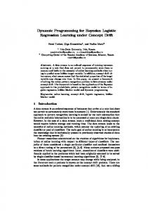
The convergence rate, the variance in trials, as vertical bars, and the completion time, as filled circles, of all algorithms are shown in Figure 4. The RRT∗ algorithm has the slowest convergence rate and the largest variance, and the RRT# 3 algorithm has the fastest convergence rate and the smallest variance in the trials. A video of the animation of the 6DOF and 12DOF cases shown in Figures 3 and 5 can be found in http://www.youtube.com/oarslan3.
Fig. 5: Initial and goal configurations of HUBO (12D) D. Motion Planning for Dual-Arm Manipulation (12 DoFs) Fig. 3: Initial and goal configurations of HUBO (6D) C. Motion Planning for Single-Arm Manipulation (6 DoFs) In this section, we test all algorithms on planning problems in high-dimensional search spaces. First, we simulate a simple workspace in which there are a table and two boxes along with a humanoid robot (HUBO), as shown in Figure 3. At the initial step, the HUBO is at rest with its right arm on one side of the two boxes, and is tasked to move its right arm to the other side of the boxes as, shown in the left-most and right-most subfigures of Figure 3, respectively. TABLE I: Results for Single-Arm Planning Problem Solution Time (s) Cost (rad) Time (s) Final Cost (rad) # of Vertices First
RRT∗ 15.38 (7.45) 6.22 (2.20) 1316.67 (338.89) 5.43 (2.20) 4360.17 (121.83)
RRT# 14.26 (7.71) 4.55 (1.49) 1187.92 (270.23) 2.60 (0.36) 4237.25 (84.36)
RRT# 1 13.88 (7.48) 4.56 (1.71) 1195.90 (283.00) 2.65 (0.43) 3394.96 (433.75)
RRT# 2 13.84 (6.97) 4.67 (1.69) 1079.40 (249.38) 2.65 (0.42) 2256.34 (235.21)
RRT# 3 13.81 (6.52) 4.63 (1.48) 675.39 (122.59) 2.62 (0.35) 1572.20 (292.14)
A Monte-Carlo study was performed in order to compare the convergence rate and variance for all algorithms. All algorithms were run for 5,000 iterations and their results were averaged over 100 trials. The averaged results of all algorithms are summarized in Table I. As seen below, the RRT# algorithm and its three variants outperformed the RRT∗ algorithm in all cases at finding the lower-cost path. Among all of them, the RRT# 3 is the fastest algorithm and computes the best solution in a much shorter amount of time.
In the final set of simulations, we tested all algorithms for a planning problem in a 12D search space. At the initial step, both arms of the HUBO lie on each side while it is standing, and then the HUBO is commanded to move its right and left arms to pre-grasp poses for the stick and steering wheel, respectively, as shown in Figure 5. TABLE II: Results for Dual-Arm Planning Problem Solution Time (s) First Cost (rad) Time (s) Final Cost (rad) # of Vertices
RRT∗ 111.47 (45.17) 10.57 (2.12) 6390.98 (714.09) 9.72 (3.71) 22470.14 (571.40)
RRT# 108.73 (48.22) 6.71 (1.70) 5455.71 (610.22) 4.96 (0.84) 21347.72 (351.74)
RRT# 1 107.42 (43.14) 6.65 (1.76) 4811.12 (305.10) 4.93 (0.78) 16147.81 (315.77)
RRT# 2 103.14 (44.37) 6.67 (1.62) 4170.12 (272.15) 4.94 (0.72) 8451.78 (307.97)
RRT# 3 100.07 (40.71) 6.59 (1.45) 2457.38 (221.71) 4.92 (0.67) 6187.18 (312.15)
A Monte-Carlo study is performed in order to compare the convergence rate and variance in the trials of all algorithms. All algorithms were run for 20,000 iterations, and their results were averaged over 25 trials. The averaged results for all algorithms are summarized in Table II. The RRT# and its variant algorithms outperform the RRT∗ algorithm at finding lower-cost paths at the final iteration on average. Among them, the RRT# 3 is the fastest algorithm, and computes the best solution in a much shorter amount of time. The convergence rate, the variance in trials, as vertical bars, and the completion time, as filled circles, of all algorithms are shown in Figure 6. Among them, the RRT∗ algorithm has the slowest convergence rate and the largest variance in the trials. The RRT# 3 algorithm has the fastest convergence rate and the smallest variance.
10
10
10
10
8
8
8
8
6
6
6
6
4
4
4
4
2
2
2
2
0
0
0
0
−2
−2
−2
−2
−4
−4
−4
−4
−6
−6
−6
−6
−8
−8
−8
−10 −10
−8
−6
−4
−2
0
2
4
6
8
10
(a)
10
−10 −10
−8
−6
−4
−2
0
2
4
6
8
10
(d)
10
−8
−10 −10
−8
−6
−4
−2
0
2
4
6
8
10
(g)
10
−10 −10
8
8
8
8
6
6
6
6
4
4
4
4
2
2
2
2
0
0
0
0
−2
−2
−2
−2
−4
−4
−4
−4
−6
−6
−6
−6
−8
−8
−8
−10 −10
−8
−6
−4
−2
0
2
4
6
8
10
(b)
10
−10 −10
−8
−6
−4
−2
0
2
4
6
8
10
(e)
10
−8
−6
−4
−2
0
2
4
6
8
10
(h)
10
−10 −10
8
8
8
6
6
6
4
4
4
4
2
2
2
2
0
0
0
0
−2
−2
−2
−2
−4
−4
−4
−4
−6
−6
−6
−6
−8
−8
−8
−6
−4
−2
0
2
4
6
8
10
−10 −10
−8
−6
−4
−2
(c)
0
2
4
(f)
6
#
8
10
−2
0
2
4
6
8
10
2
4
6
8
10
2
4
6
8
10
(j)
−8
−6
−4
−2
0
(k)
−8
−10 −10
RRT# 1 ,
−4
10
6
−8
−6
−8
−10 −10
8
−10 −10
−8
10
−8
−6
−4
RRT# 2
−2
0
(i)
2
4
6
RRT# 3
8
10
−10 −10
−8
−6
−4
−2
0
(l)
Fig. 1: The evolution of the tree computed by RRT , and algorithms is shown in (a)-(c), (d)-(f), (g)-(i) and (j)-(l), respectively. The configuration of the trees (a), (d), (g) and (j) is at 250 iterations, (b), (e), (h) and (k) is at 2500 iterations, and (c), (f), (i) and (l) is at 25000 iterations. 14 RRT* RRT#
12
RRT#1
Cost [rad]
10
RRT#2 RRT#3
8 6 4 2 0
0
1000
2000
3000
4000 Time [s]
5000
6000
7000
Fig. 6: The convergence rate of the algorithms in 12D
VI. C ONCLUSIONS AND F UTURE W ORK Three extensions of the RRT# algorithm, initially proposed in [3], are presented and their performance is compared with the RRT# algorithm both in terms of convergence rate to optimal solution and the variance in trials. The behaviors of the proposed algorithms, e.g., growth of the tree, and vertex rejection, are first shown on two 2D problems (an “easy” one and a “pathological” scenario), and then all algorithms are benchmarked using two more challenging pathplanning problems in high dimensional search spaces. Owing to the design of the RRT# algorithm, the search space is naturally decomposed into promising and non-promising vertices once an initial solution is computed. The proposed algorithm utilizes this information and uses simple rejection criteria to control the growth of the search tree and to avoid
branching off into unfavorable regions. This leads to a natural non-uniform sampling that is naturally adapted to the specific problem at hand. The simulation results demonstrate that the proposed algorithms store a fewer number of vertices in the tree, yet they compute lower cost solutions than those of the RRT∗ or the RRT# algorithm much faster. The work in this paper can be extended along several directions. Since it is crucial for the algorithm to reach the target set as early as possible in order to converge to the optimal solution faster, a bi-directional version of the proposed algorithm can be developed in order to shorten the first time-to-connect to the goal set. Also, a parallel version of the algorithms could be implemented by running the Extend and Replan procedures as separate threads. A possible implementation would be to have multiple threads implementing the Extend procedure and a single thread implementing the Replan. ACKNOWLEDGEMENTS The authors are grateful to late Prof. Mike Stilman and to the students of Humanoid Robotics Lab at Georgia Tech for providing support on how to use the GRIP + DART software platform. This work has been supported in part by ARO MURI award W911NF-11-1-0046 and ONR award N0001413-1-0563.
10
10
10
10
8
8
8
8
6
6
6
6
4
4
4
4
2
2
2
2
0
0
0
0
−2
−2
−2
−2
−4
−4
−4
−4
−6
−6
−6
−6
−8
−8
−8
−10 −10
−8
−6
−4
−2
0
2
4
6
8
10
(a)
10
−10 −10
−8
−6
−4
−2
0
2
4
6
8
10
(d)
10
−8
−10 −10
−8
−6
−4
−2
0
2
4
6
8
10
(g)
10
−10 −10
8
8
8
8
6
6
6
6
4
4
4
4
2
2
2
2
0
0
0
0
−2
−2
−2
−2
−4
−4
−4
−4
−6
−6
−6
−6
−8
−8
−8
−10 −10
−8
−6
−4
−2
0
2
4
6
8
10
(b)
10
−10 −10
−8
−6
−4
−2
0
2
4
6
8
10
(e)
10
−8
−6
−4
−2
0
2
4
6
8
10
(h)
10
−10 −10
8
8
8
6
6
6
4
4
4
4
2
2
2
2
0
0
0
0
−2
−2
−2
−2
−4
−4
−4
−4
−6
−6
−6
−6
−8
−8
−8
−6
−4
−2
0
2
4
6
8
10
−10 −10
(c)
−8
−6
−4
−2
0
(f)
2
4
6
#
8
10
−2
0
2
4
6
8
10
2
4
6
8
10
2
4
6
8
10
(j)
−8
−6
−4
−2
0
(k)
−8
−10 −10
RRT# 1 ,
−4
10
6
−8
−6
−8
−10 −10
8
−10 −10
−8
10
−8
−6
−4
RRT# 2
−2
0
(i)
2
4
6
RRT# 3
8
10
−10 −10
−8
−6
−4
−2
0
(l)
Fig. 2: The evolution of the tree computed by RRT , and algorithms is shown in (a)-(c), (d)-(f), (g)-(i) and (j)-(l), respectively. The configuration of the trees (a), (d), (g) and (j) is at 250 iterations, (b), (e), (h) and (k) is at 2500 iterations, and (c), (f), (i) and (l) is at 25000 iterations.
R EFERENCES [1] B. Akgun and M. Stilman. Sampling heuristics for optimal motion planning in high dimensions. In IEEE/RSJ International Conference on Intelligent Robots and Systems (IROS), pages 2640–2645, 2011. [2] O. Arslan, E. A. Theodorou, and P. Tsiotras. Information-theoretic stochastic optimal control via incremental sampling-based algorithms. In IEEE Symposium on Adaptive Dynamic Programming and Reinforcement Learning (ADPRL), pages 1–8, 2014. [3] O. Arslan and P. Tsiotras. Use of relaxation methods in samplingbased algorithms for optimal motion planning. In IEEE International Conference on Robotics and Automation (ICRA), pages 2413–2420, 2013. [4] D. P. Bertsekas. Dynamic Programming and Optimal Control, volume 1. Athena Scientific, Belmont, MA, 2000. [5] D. P. Bertsekas and J. Tsitsiklis. Parallel and Distributed Computation: Numerical Methods. Athena Scientific, Belmont, Massachusetts, January 1997. [6] H. Choset, K. Lynch, S. Hutchinson, G. Kantor, W. Burgard, L. Kavraki, and S. Thrun. Principles of Robot Motion: Theory, Algorithms, and Implementations. The MIT Press, 2005. [7] E. W. Dijkstra. A note on two problems in connexion with graphs. Numerische mathematik, 1(1):269–271, 1959. [8] B. Donald, P. Xavier, J. Canny, and J. Reif. Kinodynamic motion planning. Journal of the Association for Computing Machinery, 40(5):1048–1066, November 1993. [9] D. Ferguson and A. Stentz. Anytime RRTs. In IEEE/RSJ International Conference on Intelligent Robots and Systems (IROS), pages 5369– 5375, 2006. [10] J. D. Gammell, S. S. Srinivasa, and T. D. Barfoot. Informed RRT*: Optimal sampling-based path planning focused via direct sampling of an admissible ellipsoidal heuristic. In IEEE/RSJ International Conference on Intelligent Robots and Systems (IROS), pages 2997– 3004, 2014. [11] P. E. Hart, N. J. Nilsson, and B. Raphael. A formal basis for the
[12]
[13] [14] [15]
[16]
[17] [18] [19] [20] [21] [22]
heuristic determination of minimum cost paths. IEEE Transactions on Systems Science and Cybernetics, 4(2):100–107, 1968. V. A. Huynh, S. Karaman, and E. Frazzoli. An incremental samplingbased algorithm for stochastic optimal control. In IEEE International Conference on Robotics and Automation (ICRA), pages 2865–2872, 2012. S. Karaman and E. Frazzoli. Incremental sampling-based algorithms for a class of pursuit-evasion games. In Algorithmic Foundations of Robotics IX, pages 71–87. Springer, 2011. S. Karaman and E. Frazzoli. Sampling-based algorithms for optimal motion planning. International Journal of Robotics Research, 30(7):846–894, 2011. L. E. Kavraki and J.-C. Latombe. Randomized preprocessing of configuration space for fast path planning. Technical Report STANCS-93-1490, Dept. Computer Science, Stanford University, Stanford, CA, 1993. ˇ L. E. Kavraki, P. Svestka, J.-C. Latombe, and M. H. Overmars. Probabilistic roadmaps for path planning in high-dimensional configuration spaces. IEEE Transactions on Robotics and Automation, 12(4):566– 580, 1996. S. Koenig and M. Likhachev. D∗ lite. In Eighteenth National Conference on Artificial Intelligence, pages 476–483, Menlo Park, CA, 2002. American Association for Artificial Intelligence. S. Koenig and M. Likhachev. Fast replanning for navigation in unknown terrain. IEEE Transactions on Robotics, 21(3):354–363, 2005. S. Koenig, M. Likhachev, and D. Furcy. Lifelong planning A*. Artificial Intelligence Journal, 155(1-2):93–146, 2004. S. M. LaValle. Planning Algorithms. Cambridge Univ Pr, 2006. S. M. LaValle and J. J. Kuffner, Jr. Randomized kinodynamic planning. International Journal of Robotics Research, 20(5):378–400, May 2001. M. Otte and N. Correll. C-FOREST: Parallel shortest path planning with superlinear speedup. IEEE Transactions on Robotics, 29(3):798– 806, 2013.