Acta Polytechnica Hungarica
Dynamic Resource Allocation in Cloud Computing Seyedmajid Mousavi1, Amir Mosavi2,3,4, Annamria R. VarkonyiKoczy2,5, Gabor Fazekas1 1
Faculty of Informatics, University of Debrecen, Kassai Str. 26, 4028 Debrecen, Hungary, {majid.mousavi & fazekas.gabor}@inf.unideb.hu 2
Institute of Automation, Kando Kalman Faculty of Electrical Engineering, Obuda University, Becsi Str. 94-96, 1431 Budapest, Hungary,
[email protected],
[email protected] 3
Norwegian University of Science and Technology, Department of Computer Science, 7491 Trondheim, Norway 4
Institute of Structural Mechanics, Bauhaus Universität-Weimar, Marienstraße 15, 99423 Weimar, Germany 5
Department of Mathematics and Informatics, J. Selye University, Elektrarenska cesta 2, 945 01 Komarno, Slovakia
Abstract: Utilizing dynamic resource allocation for load balancing is considered as an important optimization process in cloud computing. In order to achieve maximum resource efficiency and scalability in a speedy manner this process is concerned with multiple objectives for an effective distribution of loads among virtual machines. In this realm, exploring new algorithms, as well as development of novel algorithms, is highly desired for technological advancement and continued progress in resource allocation application in cloud computing. Accordingly, this paper explores the application of two relatively new optimization algorithms and further proposes a hybrid algorithm for load balancing which can contribute well in maximizing the throughput of the cloud provider's network. The proposed algorithm is a hybrid of teaching-learning-based optimization algorithm (TLBO) and grey wolves optimization algorithm (GW). The hybrid algorithm performs more efficiently than utilizing every single one of these algorithms. Furthermore, it well balances the priorities and effectively considers load balancing based on time, cost, and avoidance of local optimum traps, which consequently leads to minimal amount of waiting time. To evaluate the effectiveness of the proposed algorithm, a comparison with the TLBO and GW algorithms is conducted and the experimental results are presented.
–1–
Mousavi et al.
1
Dynamic Resource Allocation in Cloud Computing
Introduction
A cloud is created from numerous physical machines. Each physical machine runs multiple virtual machines which are presented to the end-users, or so-called clients, as the computing resources. The architecture of virtual machines is based on physical computers with similar functionality. In cloud computing, a virtual machine is a guest program with software resources which works like a real physical computer [1]. Yet, high workload on virtual machines is one of the challenges of cloud computing in the allocation of virtual machines. The task, requested by a client, has to wait to be allocated to the work and the resources needed. This strategy is independent of the executive priority of the tasks. However, the client who owns the task may offer larger value for it to try to raise his/her priority and eventually may succeed in taking control over the resources needed. Users can consume services based on the service level agreement that defines their needs of quality of service (QoS) parameters [2]. Yet, the multipurpose nature of the scheduling in the cloud computing environment has made it extremely difficult to manage. Therefore, scheduling has to create a compromise between service quality costs to come up with a suitable service which belongs to a multi-objective optimization problems family [3]. Several methods are available for a multi-objective scheduling problem [4]. The current methods of allocation of resources, such as FIFO [1] and Round-Robin [5] which are used in the cloud, do unfair allocation regardless of priority between tasks. Resource allocation in the cloud environment is utilized to achieve customer satisfaction with minimal processing time. Reducing the fees of leasing resources in addition to ensuring quality of service and improving throughput for trust and satisfaction of the service provider is considered as another objective. In dynamic scheduling, the basic idea is the request allocation at the time of implementation of programs. In addition to the cost estimation, in the static method, dynamic scheduling consists of two other main sections of system state estimation and decision-making [6]. To recap, clients are interested in having their tasks completed in the shortest possible time and at the minimum cost which cloud servers should receive. On the other hand, the cloud providers are interested to maximize the use of their resources and also to increase their profits. Obviously these two objectives are in conflict with each other and often they are not satisfied with the traditional methods of resource allocation and scheduling mechanisms available [7]. Yet the goal is to direct the resource allocation to be performed in a way that is acceptable to both the users and the suppliers. Resource allocation is a technique that ensures the allocation to virtual machines when multiple applications need different resources of CPU and input/output memory [2]. In cloud computing there are two technical restrictions. Firstly, the capacity of the machines is physically limited; secondly, priorities for the implementation of the tasks should be in harmony with maximizing the efficiency of resources. Ultimately, the waiting time and the completion time are to be
–2–
Acta Polytechnica Hungarica
reduced, in order to decrease the cost of system implementation. Classical methods for achieving a fully optimized solution are very time-consuming and in some cases are impossible. Traditional approximate methods [5] are reported inconclusive and inaccurate for solving optimization problems and are often trapped in local optimum. Virtual machines in distributed systems have different usage conditions including; the cost of utilizing them and also different processing power. The tasks initiated by users may also have a different amount of information. In addition, to assign any task on any machine, a preparation time between tasks is also considered. This time-delay, which varies in different resources, is considered negligible in this study. The most important problem in this process is the order process and how the placement of tasks on resources is conducted. In fact by increasing the productivity of resources, the response time can be reduced and, simultaneously, can improve the total cost for resource utilization and load balancing. The loadbalancing index is calculated based on target variables. The target variables include: The time of completing the latest task among virtual machines The average cost paid by the user for use of the resources Efficiency caused by the impact of load balancing based on completion time and cost of doing them. To conduct this study in the realm of cloud computing system development, a number of assumptions are made with the following characteristics. In these assumptions, the resource and virtual machine are considered as one entity. Tasks are independent. Distributed environment is heterogeneous and dynamic. All tasks must be done. Each task is performed only by one virtual machine. Everything is done exactly once. Each virtual machine has different and specified processing speed. Each virtual machine has a special price that must be paid for the use of it in time. Traditional approximation and resource allocation methods (see, e.g. [7]) due to the multi-objective and dynamic nature of the problem and also difficulties in dealing with local optimum need advancement and major improvement. Consequently, the purpose of this paper is set to address the research gap in cloud computing. To do so a hybrid approximation algorithm for resource allocation is proposed. In this study the performance of two algorithms i.e. teaching-learningbased optimization (TLBO) [8] and grey wolves optimization (GW) [9], in comparison with the proposed algorithm, are discussed. These two algorithms are currently used as approximation algorithms for establishing load balancing, based on time and cost between resources and efficiency. The balance is established between three target assessment variables for evaluating the proposed approximation algorithm.
–3–
Mousavi et al.
2
Dynamic Resource Allocation in Cloud Computing
Related Works
For resource allocation in distributed scheduling, Xu et al. [5] present a nondominated sorting genetic algorithm-based multi-objective method (NSGA-II) [10]. They aimed at minimizing the time and cost in load balancing using resources to achieve Pareto optimal front. They used self-adaptive crowding distance (SCD) to overcome the crowding distance. In addition, in their proposed method, a mutation operator is included in the traditional algorithm of NSGA-II to avoid premature convergence. In this method, the strategy that the algorithm uses for improving the efficiency and performance of the intersections, has not been effective, as the solutions are trapped in local optimum. Salimi et al. [14] introduced a multi-objective tasks’ scheduling using fuzzy systems and standard NSGA-II algorithms for distributed computing systems in [6]. The authors aimed at minimizing implementation time and costs while increasing the productivity of resources. Their study is associated with the load balancing in the distributed system. They use the indirect method and fuzzy systems and do implementation of the third objective function to solve this problem. However dealing with three objectives has not been efficiently done in their work. In [7], Cheng provides an optimized hierarchical resource allocation algorithm for workflows using a general heuristic algorithm. In this model, the main objective is the coordination between the tasks and duties assigned to the service. The purpose is to service in accordance with the operational needs to perform properly the tasks and observe the priority between them. This model accomplishes workflow tasks scheduling aimed at load balancing by(?) dividing the tasks to different levels. Further, mapping and allocation of each level of tasks to resources is directed according to the processing power. Gomathi and Karthikey [8] introduce a method for assigning tasks in a distributed environment using Hybrid Particle Swarm Optimization algorithm (HybPSO) [11]. HybPSO is used to meet the user needs and increase the amount of load balancing with productivity. The goal is to minimize the task completion time among processors and create load balancing. This method assures that each task is assigned to exactly one processor. In this method, each solution is shown as a particle in the population; each particle is a vector with n dimension which is defined for scheduling n independent tasks. In [9], authors introduce a heuristic method based on particle swarm algorithm [12] for tasks’ scheduling on distributed environment resources. Their model considers the computational cost and the cost of data transfer. Their proposed algorithm optimizes dynamic mapping tasks to resources using classical particle swarm optimization algorithm and ultimately balances the system loads. This optimization method is composed of two components. One of them is the scheduling operations task and the other one is particle swarm algorithm (PSA) to obtain an optimal mix of the tasks to resources’ mapping.
–4–
Acta Polytechnica Hungarica
Table1 presents a summary of the related works done in the field of tasks’ scheduling. This table includes the objectives of tasks’ scheduling, the algorithms used in these methods, the simulation environment of the algorithms, and the year in which they were developed. Table1 does not include the GW and educationbased learning algorithms and/or any variations of these algorithms. Table1 Summary of the works done in the field of resources’ allocation Author
Evolutionary Environment algorithm
Xue et al [13]
multi-target genetic
Cloud
Salimi et al [14]
multi-target genetic
Grid
Cheng [15]
genetic
Cloud
Gomathi & Karthikey [8]
swarm optimization
Cloud
Pandey et al [17]
swarm optimization
Cloud
Wu et al [18]
swarm optimization
Grid
Izakian et al [19]
swarm optimization
Cloud
Banerjee et al [20]
Ant colony
Cloud
Mousavi & Fazekas [21]
Ant colony
Cloud
Ludwig & Moallem [22]
Ant colony
Grid
Bee colony
Cloud
swarm optimization
Cloud
Simulated Annealing
Cloud
Babu & Krishna [23]
Zhao [24] Abdullah & Othman [25]
Targets Reduce the longest termination time among resources Reduce the resources cost Load balancing Reduce the longest termination time among resources Reduce the resources cost Load balancing Reduce the longest termination time among resources Load balancing Reduce the longest termination time among resources Load balancing Reduce costs associated with load balancing Reduce the longest termination time among resources Reduce the workflow time Load balancing Reduce the longest termination time among resources Reduce the workflow time Load balancing Reduce the longest termination time among resources Load balancing Reduce the longest termination time among resources Reduce the workflow time Load balancing Reduce the longest termination time among resources Load balancing Reduce the longest termination time among resources Load balancing Reduce the longest termination time among resources Reduce the resources cost Reduce the longest termination time among resources Load balancing
Year
Simulation tool
2014
Matlab
2014
GridSim
2012 Java environment
2013 Java environment 2010
Amazon EC2
2012
Ad-hoc VC++ toolkit
2010
Java environment
2009
Simulated cloud
2016
CloudSim
2011
GridSim
2013
CloudSim
2015
CloudSim
2014
CloudSim
The literature review shows that traditional methods which are used for optimization, may be definitive and accurate, yet they are often trapped in local optimum. In fact, due to the dynamic nature of distributed environment and –5–
Mousavi et al.
Dynamic Resource Allocation in Cloud Computing
heterogeneous resources, in such a system, the scheduling process must be done automatically and very quickly. That is why the scheduling process is recognized as an NP-complete problem [26]. Traditional approaches are not dynamic and suitable to solve such a scheduling problem. These approaches contain a large search space; facing a large number of possible solutions and a tedious process to find the optimal solution. There is currently no efficient method available to solve these problems. In such circumstances, the traditional approach has been set to find a fully optimized solution instead of finding the semi-optimal solution, but in a shorter time. In this context, IT professionals are focused on exploratory methods. Therefore, metaheuristic algorithms which have a global overview, as they ensure convergence to solution and do not fall into the trap in local optimum, are of importance. Consequently, the GW algorithm is chosen for this purpose. In addition, the TLBO algorithm is used in a hybrid form with GW to improve local optimization and increase accuracy.
3
Proposed method
Methodology is based on bonding the algorithms of TLBO and GW. With such hybridization, it is aimed at speeding up the process while maintaining the improvement of local optimization and increasing the accuracy. In the following, the problem is described. Further TLBO and GW algorithms are introduced as the primary solutions to the described problem. The proposed methodology then emerges from bonding of two algorithms.
3.1
Description of the Problem
There is a distributed network in a cloud environment with resource systems S1,S2,S3,…,Sn. The resources are ready to serve in the distributed network for various nodes. Different jobs are sent for the source systems by nodes. The overall goal of this system is that, an agreed scheduling on the resources’ allocation is to be obtained to perform the jobs. Consequently, with the resources allocation, the load balancing will be increased [27]. Here the scheduler is responsible to allocate one or more jobs to artificial machines in a distributed system [28]. In other words, the agreement on job scheduling is done by the scheduler. The scheduler provides a scheduling for resource allocation [29]. Several jobs are allocated and processed in parallel with each other at time - t - in the distributed system. The number of variables Tk is permutation between jobs and resources, this variable is called P, and its value is calculated as follows:
P
–6–
nm
n is number of tasks and m is the number of sources
(1)
Acta Polytechnica Hungarica
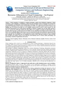
As it is described in Figure 1 each node includes several jobs. Each job requires a series of specific resources. The problem can be introduced as Job j1,j2,…,jn and Resource R1,R2, … , Rm .
Figure 1. Resource allocation in a distributed environment
If in the particular example, the resources R1,R2, … , Rm have the same capacity and processing power and j1,j2,…,jn all need 1% of the processing. The advanced model can be defined in a form describing what jobs in which resources should be used in order to achieve the maximum load balancing, average response time, and minimum cost. For the exact solution of the problem, all possible allocation modes must be calculated and the best mode chosen. Due to the large number of modes (exponential), the problem is an example of set packing problems, which is of NP-complete type. Optimization function is defined for resource i and job j. yi is the number of resources (package). The objective function and mathematical programming model that should be optimized are as follows:
Min B
a * 1 L( y j )
b *C ( y j )
c *T ( y j )
(2)
S.t. n
n
wixi j i 1
Ky j , j ,
xi j
bj , j
xi j ,yi
0,1
i, j
j 1
Where :
xj
1
job j is used
0
job j isnot used
, yj
1 resource j is used 0 resource j isnot used
xi j represents that job j is assigned to resource i. C is the maximum capacity for each resource. wi represents the amount of job i that is covered by the resource. The aim is to find the minimum number of virtual machines - Yj - that minimize the objective functions. The values of L, C, and T (load balancing, cost, and response time) are considered based on the number of virtual resources, Yj, where
–7–
Mousavi et al.
Dynamic Resource Allocation in Cloud Computing
a, b, c are variable based on cloud system. The variable of Xij demonstrates that the ith job is in jth virtual machines, and if its value is equal to 0, it means that there is not any resource in jth virtual machine and if its value is equal to 1, it means that there is enough resource to allocate the jth virtual machine. Every job has the capacity of Wi. The first limitation indicates that total capacity of jobs can be placed at the maximum - K - available resources. The second limitation shows the maximum capacity of each virtual resource. bj is the capacity of each virtual resource.
3.2
Grey wolf algorithm
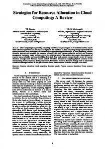
Mirjalili et al. [30] introduce GW for solving engineering problems. GW is a new optimization algorithm inspired by behavior of grey wolves’ hunting and their role hierarchies. The GW algorithm is benchmarked on 29 well-known test functions and the results on the unimodal functions show the superior exploitation of GW. Capability of exploration of new solutions in GW algorithm is confirmed by the results of multimodal function. The hierarchical structure and social behavior of wolves during the hunting process is modeled in the form of mathematical models and is used to design an optimization algorithm. The GW optimization algorithm emulates the hierarchical leadership and hunting mechanism of Grey Wolves in nature. Four types of GWs are considered as hierarchical structure in the social behavior of wolves for simulating, such as alpha, beta, delta, and omega. Furthermore, the three main steps of hunting - searching for prey, encircling prey, and attacking prey are implemented (figure 2).
Figure 2. Grey wolves’ motion in haunting [30]
–8–
Acta Polytechnica Hungarica
Figure 3. Updating wolves' position [30]
The Wolves’ leader is called alpha and is primarily responsible for the prey. The second level of wolves, which helps the leader, is called beta. The third level of wolves is called delta and is designed to support alpha and beta. The lowest level is called Omega [31]. In general, the algorithm steps can be summarized as follows: The fitness of all solution levels are computed and three top solutions are selected as Alpha, Beta, and Delta (Figure 2) until the end of the algorithm. In fact, Alpha is the best fitness of solution. After Alpha, the Beta and Delta are the best solutions respectively. In each iteration, the three top solutions e.g. Alpha, Beta, and Delta have the ability to estimate the prey position, conducting it in each iteration using the following equations [30]: (3)
D α = C 1 .X α -X , D β = C 2 .X β -X , D δ = C 3 .X δ -X
X (t
1)
X1
X2 3
X
3
where
X X X
1 2 3
X X X
A 1.( D ) A 2 .( D ) A 3 .( D )
(4)
First, the wolves put a ring around the prey, where Xp, is the hunting position vector. A and C are hunting vector coefficients. X is the wolves' positions and t stands for the stage of each iteration. D indicates the behavior of putting the ring around the hunt [30]. In each iteration, after determining the positions of Alpha, Beta, and Delta, the other solutions are updated in compliance with them. Hunting –9–
Mousavi et al.
Dynamic Resource Allocation in Cloud Computing
information is defined by Alpha, Beta, and Delta. And the rest update their x positions accordingly. In each iteration, vector and consequently vectors b and c are updated. At the end of an iteration, Alpha wolf position is considered as the optimal point. This value is A. A value of A is an option value which is between (2a, 2a). The absolute value of A is less than 1, so when the wolves are at the A distance from the prey, attack happens. At a distance of more than one, it is still(??) necessary that the wolves must converge toward each other [4]. In the GW algorithm, some main parameters like initial population size, vector coefficients, number of iterations, and the number of wolf levels are to be determined [32]. Then, the cost function of optimization which is minimized in this study is introduced. Afterward, the initial population is formed randomly and the fitness function is introduced. Then, in a loop on a regular basis, the position of the wolves' level is determined and the fitness function is calculated, and, using them, the new positions are calculated again. Iteration of this loop is specified according to the initial parameters.
3.3
Teaching-learning-based algorithm
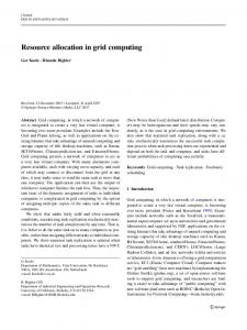
Teaching-learning-based optimization algorithm (TLBO) [33] provides a novel approach to explore a problem space to find the optimal settings and parameters to satisfy the problem’s objectives. The algorithm was introduced by Rao et al [33]. Similar to other evolutionary optimization techniques, TLBO algorithm is an algorithm derived from nature and works based on a teacher’s teaching in a classroom. A teacher in the classroom, by expressing material, plays an important role in student learning and, if the teaching is effective, students learn the material better. In addition to the teacher factor, review of lessons by students would lead to better learning. This algorithm uses a total population of solutions to achieve the overall solution. A teacher tries to increase the level of students’ knowledge by teaching and repeating the materials. Therefore the students can achieve a good score. In fact, a good teacher makes students closer to the level of his/her knowledge. The teacher is the most knowledgeable person of the class that shares his/her knowledge with the students. So the best solution (the best student of the class population) in the same iteration can act as a teacher. It should be considered that the students acquire knowledge based on the quality of teaching by the teacher and students’ status (the average of class scores). This idea is the basis of Teaching-Learning-Based Optimization algorithm for solving optimization problems. The algorithm operates in two phases. The first phase is the teacher who shares his/her knowledge with students and the second phase is the review of courses by students in the same class. At the first stage, a teacher tries to improve scores of a class. In Figure 4, the Gaussian distribution function is used and the average scores acquired by students in the classroom is shown as M. M Parameter indicates the degree of the teacher’s success in the classroom. In this figure, M1 and M2, respectively, show average scores of two separate classrooms with the same students.
– 10 –
Acta Polytechnica Hungarica
M1
M2
MA
Curve 1 Curve 2
MB
Curve A Curve B
.
TA
.
TB
Figure 4. Average scores of students who were in classroom [33]
As it is shown in figure 4, the second teacher, with average scores of M2, has acted better than the first teacher with average score of M1. TA is the first grade teacher, who, with the best-case average scores of the first grade, MA, moves to the TA. It means that the academic level of students is approaching that of their teacher or equal with him/her. This creates a new population of the classroom which has shown an average of MB and TB. In fact, the students do not reach the knowledge level of the teachers, just close to it, which also depends on the level of classroom ability. Gaussian probability function is defined as follow [34,36]: f (X )
1 2
)2
(x
e
2
2
(5)
In this formula, μ is the average score of students, which is shown as M1 and M2 in Figure 4.
3.4
Proposed algorithm
Given more convergence power in the global optimality, the GW algorithm is used as a base algorithm in the proposed algorithm. This algorithm can also perform multi-objective optimization. The steps are as follows. In the initial state, a series of random numbers as the initial population are considered with uniform distribution and a basic solution is considered for the problem. Coefficients a, b, and c are initialized. Each solution is known as a wolf. In another word, each wolf is considered as a solution to the problem. These solutions or wolves have an answer. Wolves are divided into three categories; alpha, beta, and gamma. Yet on the basis of the fitness function, one of them gives a better answer to the fitness function. Then, the solution enters the main loop where after a few iterations the best solution for the fitness function is discovered. Based on the equations of the GW algorithm, the wolves' position is updated. According to the first class of wolves, the new positions are fitted. Later on, more values for the probability of solution are considered. Correspondingly, the values of beta and gamma classes, the new positions of wolves, and their classifications can be obtained. If a suitable solution is found in the new classification, the algorithm is to be improved further. The best solution between the wolves is considered as the initial solution (initial population) for the teaching and learning algorithm. Further, the problem of the teaching and learning algorithm is solved – 11 –
Mousavi et al.
Dynamic Resource Allocation in Cloud Computing
and the solution is considered as initial population to start again. In this stage the GW algorithm is implemented. If there is no improvement in GW algorithm, according to the teaching and learning, it tries to find a better solution. If the solution is trapped in local optimum, an algorithm based on teaching and learning can introduce the new area of space based on training, which may improve solution. Since the accuracy of GW algorithm in the local behaviour is high, after each stage the position of wolves is determined. This position can be improved by learning and training algorithms, and GW algorithm is implemented again. This process increases the accuracy of GW algorithm. It should be considered that in the GW algorithm, every wolf represents a solution in the solution space. The best and the most successful solution will be chosen among them at any stage according to the position of other wolves. The best solution of the GW is defined as the initial solution for teaching and learning. After learning and training, its output is implemented as the initial solution for the next iteration in the GW algorithm. The proposed algorithm is presented in table 2: Table 2 Pseudo code of the proposed algorithm
Initialize the grey wolf population Xi=(i=1,2,…,n) Initialize a,b and c Calculate the fitness of each search agent X1=the best Search gent X2=the second best Search Agent X3=the third best Search agent While t