Dynamic Routing Schemes for Graphs with Low Local ... - CiteSeerX

Dynamic Routing Schemes for Graphs with Low Local Density

Amos Korman

∗

David Peleg

†

March 12, 2007 Abstract This paper studies approximate distributed routing schemes on dynamic communication networks. The paper focuses on dynamic weighted general graphs where the vertices of the graph are fixed but the weights of the edges may change. Our main contribution concerns bounding the cost of adapting to dynamic changes. The update efficiency of a routing scheme is measured by the time needed in order to update the routing scheme following a weight change. A naive dynamic routing scheme, which updates all vertices following a weight change, requires Ω(Diam) time in order to perform the updates after every weight change, where Diam is the diameter of the underlying graph. In contrast, this paper presents approximate dynamic routing schemes with average time complexity ˜ Θ(D), per topological change, where D is the local density parameter of the underlying graph. Following a weight change, our scheme never incurs more than Diam time, thus, our scheme is particularly efficient on graphs which have low local density and large diameter. The paper also establishes upper and lower bounds on the size of the databases required by the scheme at each site.

∗

Information Systems Group, Faculty of IE&M, The Technion, Haifa, 32000 Israel. E-mail: [email protected]. Supported in part at the Technion by an Aly Kaufman fellowship. † Department of Computer Science and Applied Mathematics, The Weizmann Institute of Science, Rehovot, 76100 Israel. E-mail: [email protected]. Supported in part by grants from the Israel Science Foundation and the Israel Ministry of Science and Art.

1

Introduction

Motivation: The basic function of a communication network, namely, message delivery, is performed by its routing scheme. Subsequently, the performance of the network as a whole may be dominated by the quality of the routing scheme. Thus, constructing an efficient routing scheme is one of the most important tasks when dealing with communication network design. We distinguish between static and dynamic routing schemes. In a static routing scheme the databases of the processors are tailored to the particular network topology. However, in most communication networks, the typical setting is highly dynamic, namely, even when the physical infrastructure is relatively stable, the network traffic load patterns undergo repeated changes. Therefore, for a routing scheme to be useful in practice, it should be capable of reflecting up-to-date load information in a dynamic setting, which may require occasional updates to the databases. The communication network is modeled by an undirected connected graph. We consider the local distributed model, in which the size of the messages is unbounded (cf. [L92, P00]). The communication is asynchronous, and it is assumed that a message transmitted over a link arrives within at most one unit of time. A simple dynamic routing scheme can be constructed, which updates all vertices following each topological change. In order to perform the updates, such a scheme requires Ω(Diam) time after every weight change, where Diam is the diameter of the underlying graph. Ideally, upon a topological change, only a few time units should pass before the updates are completed. We distinguish between the average time complexity and the maximum time complexity of a dynamic scheme π on a graph G, defined as follows. Given a scenario σ of topological changes on G, the average (respectively, maximum) time complexity of π during σ is the average (resp., maximum) number of time units required by π to update the vertices following a topological change in σ. The average (respectively, maximum) time complexity of π on the graph G is the average (resp., maximum) of this value over all scenarios of topological changes in G. As shown later, the maximum time complexity of a routing scheme is Ω(Diam) in many cases, even for graphs with constant local density. We therefore concentrate on constructing dynamic routing schemes which are efficient in terms of their average time complexity. The efficiency of a dynamic scheme is measured not only by its time complexity but also by the quality of the routes it provides and by the memory complexities associated with it. Route quality is measured by the stretch factor of the scheme, i.e., the maximum ratio, over all pairs of nodes in the network, between the length of the route provided for them by the 1

routing scheme, and the actual (weighted) distance between them in the network. We focus on β-approximate routing schemes, namely, ones that produce a route whose weighted length is perhaps not the shortest possible, but approximates it by a factor of at most β, for some constant β > 1. Another consideration is the amount of information stored at each vertex. We distinguish between the internal database Data(v) used by each node v to deduce the required information in response to online queries, and the additional external storage M emory(v) at each node v, used during (offline) updates and maintenance operations. For certain applications, the internal database Data(v) is often kept in the router itself, whereas the additional storage M emory(v) is kept on some external storage device. Subsequently, the size of Data(v) is a more critical consideration than the total amount of storage needed for the information maintenance. The current paper investigates routing schemes on dynamic settings involving changing link weights. The model studied considers a network whose underlying topology is a fixed graph, i.e., the vertices and edges of the network are fixed but the (positive integer) weights of the edges may change. At each time the weight of one of the edges can increase or decrease by a fixed quanta (which for notational convenience is set to be 1), as long as the weight remains a positive integer. (Our algorithms and bounds apply also for larger weight changes, as clearly, a weight change of ∆ > 1 can be handled, albeit naively, by simulating it as ∆ individual weight changes of 1. As our focus is on establishing the complexity bounds for the problem, no attempt was made to optimize the performance of our algorithms in case of large weight changes.) We remark that it can be shown that if edge weights are also allowed to be zero, then on almost any underlying graph, the average complexity of any approximated dynamic routing scheme is Ω(Diam). Also note that if edges are allowed to be deleted and added, it is shown in [AGR89] that the average message complexity of constant approximation routing schemes on general dynamic graphs is Ω(n). This lower bound also applies for the average time complexity even on underlying graphs with constant local density, defined next. For a graph G and integer r ≥ 1, let N (v, r) denote the set of vertices at distance at most r from the node v. Then the local density parameter of G is D = maxv,r {|N (v, r)|/2r}. This graph theoretic parameter is well-studied, especially with relation to the bandwidth B of the graph G (see [F00, FT05, CCDG82, CS89, KLMN04]). In fact, it is easy to show that D ≤ B. Previous research suggests the conjecture that B = O(D log n), and it in known that B = O(D polylog n) [F00]. In this paper we present dynamic approximate routing schemes which are particularly 2

efficient on graphs which have low local density and large diameter. Specifically, our dynamic ˜ approximate routing schemes have average time complexity Θ(D) on every underlying graph with local density D. Related work: Many routing schemes and lower bounds for the resources required for routing were presented in the past (cf. [P00]). The first studies attempting to characterize and bound the resource tradeoffs involved in routing schemes for general networks were presented in [PU89, ABLP90, AP92] and were followed by a number of improved constructions (cf. [C01, IK00, IO03, TZ01]). These studies focused on routing schemes with compact routing tables and low stretch factors. Unfortunately, most of the known algorithms in this field apply only for static networks, and only a few papers consider dynamic networks. In [SK85] a partial solution is presented for limited cases of topology changes that keep the network in a tree topology. The following dynamic routing schemes on trees assume that the designer of the routing scheme has the freedom to choose the identities of the vertices. [AGR89] presents a routing scheme for the restricted case of dynamic growing trees using identities of size O(log2 n), database size O(∆ log3 n) (where ∆ is the maximum degree in the graph) and average message complexity O(log n) per topological change, where n is an upper bound on the number of vertices in the growing tree. When an upper bound n on the number of vertices in the growing tree is known in advance, a routing scheme with average message complexity O( logloglogn n ) and polylogarithmic database size is given in [KPR04]. In the more general case where in each step, a leaf can either be added to or removed from the tree, a routing scheme with O(log2 n) average message complexity and O(log2 n) database size is presented in [KPR04] and a routing scheme with Θ(log n) database size and sublinear average message complexity is presented in [K05]. All the above mentioned dynamic routing schemes deal only with tree networks. For general graphs there are even fewer results. In the case where edges may be added to or deleted from the graph, a lower bound of Ω(n) is established in [AGR89] for the average message complexity of constant approximation routing schemes on general dynamic graphs. This bound can be translated to a lower bound of Ω(n) on the average time of constant approximation routing schemes on general dynamic graphs. Moreover, this bound holds even on graphs with constant local density. In addition, another lower bound of Ω(n) is established in [AGR89] for the average message complexity of constant approximation routing schemes on growing trees, in the case where the adversary of the routing scheme chooses the identities of the vertices. The routing scheme of [DKKP95] for dynamic graphs applies to a somewhat different 3

networking model based on virtual circuits, and the route quality is measured therein in terms of the number of “super-hops” required for a route, hence those results cannot be directly compared with ours. Also, the analysis therein does not consider the length of the routes produced by the routing scheme, and in fact the scheme may incur a linear stretch factor in some dynamic scenarios. The maximum database size of β-approximate point-to-point routing schemes (defined below) on general graphs was previously investigated for the static scenario. A lower bound 1 of Ω(n 2β+4 ) for β ≥ 2 was shown in [PU89] and a lower bound of Ω(n log n) for 1 ≤ β < 2 was shown in [FG97]. In the sequential (non-distributed) model, dynamic data structures have been studied extensively. For comprehensive surveys on dynamic graph algorithms see [EGI99, FK00]. The model: In this paper the underlying network topologies considered are general graphs. Throughout the paper, denote by n the number of vertices in the network. This paper studies two types of routing schemes. Source-directed routing schemes are routing schemes in which the message originator computes the entire route to the destination and attaches it to the message header. In contrast, point-to-point routing schemes route messages on a hop by hop basis, with each intermediate node along the the route determining the next edge to be used. Formally, we make the following definitions. A point-to-point β-approximate routing scheme is composed of an update protocol for assigning each vertex v of the graph with a local database Data(v), coupled with a router algorithm whose inputs are the header of a message M , Data(v) and the identity of a vertex u. If a vertex x wishes to send a message M to vertex y, it first prepares a header for M and attaches it to M . Then, x’s router algorithm outputs a port of x on which the message is delivered to the next vertex, until it reaches y. The requirement is that the weighted length of the resulting path connecting x and y is a β-approximation of the weighted distance between x and y at the time the route starts. A source directed β-approximate routing scheme is composed of an update protocol algorithm for assigning each vertex v of a graph with a local database Data(v), coupled with a router algorithm that using only the information in Data(v) and the identity of a vertex u, outputs a sequence of port numbers representing a path connecting v and u whose weighted length is a β-approximation of the distance between u and v. Our contribution: Our main contribution focuses on the average time complexity of dynamic routing schemes. We use the local density parameter in an attempt at capturing the graph theoretic parameter governing the message complexity of the problem. 4

In section 3 we present our β-approximate source directed scheme for the class F(n, D) of n-vertex graphs with local density at most D. In section 4 we present our β-approximate point-to-point routing scheme for F(n, D). Both schemes incur an average time complexity O(D log2 n) per weight change. In terms of the database size, we show an upper bound of O(n log n) and a lower bound of Ω(n) for the database size of β-approximate source directed routing scheme on F(n, D) (for D ≥ 1.5). Our point-to-point β-approximate routing scheme uses database size O(n log2 n). The point-to-point routing scheme uses a header size of O(log n) bits.

2

Preliminaries

2.1

The dynamic network model

We assume that the vertices and edges of the network are fixed and that the edges of the network are assigned positive integer weights. An unweighted graph is a graph whose edges have unit weight. Denote by dG (u, v) the unweighted distance between u and v in G. For q > 0, the q-neighborhood of v ∈ G, denoted Γ(v, q), is the subgraph of G induced by {u | dG (v, u) ≤ q}. The subscript G can be omitted when the graph G is clear from the context. It is assumed that the nodes of a given n-vertex graph have distinct identities in the range 1, · · · , n. The identity of a node v is denoted by id(v). In the dynamic network model considered in this paper, it is assumed that the weights of the network links may change from time to time. For example, the weights may represent the current loads on the links which may change due to queue buildups and nonuniform arrival rates. For two vertices u and v in a weighted graph G with edge weight function ω and for a time t, denote by dωG (u, v, t) the weighted distance between u and v at time t. The following dynamic events may occur from time to time. 1. Positive weight change: An edge e = (u, v) increases its weight by one. 2. Negative weight change: An edge e = (u, v) with weight w(e) ≥ 2 decreases its weight by one. Subsequent to an event on an edge e = (u, v), its endpoints u and v are informed of this event.

5

2.2

Routing schemes

Static routing schemes: Let us first describe our routing schemes in the static setting. For fixed β > 1, a static β-approximate source directed routing scheme πSD = hPSD , RSD i for a family of graphs F is composed of the following components: 1. A preprocessing algorithm PSD that given a graph G ∈ F, assigns a local database Data(v) to each vertex v ∈ G. 2. A polynomial time router algorithm RSD that given the database Data(u) and id(v) for some vertices u and v in some graph G ∈ F , outputs a sequence of port numbers representing a path P connecting u and v. A static β-approximate point-to-point routing scheme πP T P = hPP T P , RP T P i for a family of graphs F is composed of the following components: 1. A preprocessing algorithm PP T P that given a graph G ∈ F , assigns a local database Data(v) to each vertex v ∈ G. 2. A polynomial time router algorithm RP T P that given the database Data(u) and id(v) for some vertices u and v in some graph G ∈ F and a header H of a message M , outputs a port number of u and a new header for M . Routing a message using a point-to-point routing scheme πP T P is done as follows. If a vertex x wants to send a message M to the vertex y in G, it first prepares a header H for M and attaches it to M . Then the message is delivered via the port RP T P (Data(x), id(y), h) to x0 , a neighbor of x. The vertex x0 repeats the process, using its own data base Data(x0 ). The message M is thus delivered on the port RP T P (Data(x0 ), id(y), h) of x0 to the next vertex and so forth. In contrast, when using a source-directed routing scheme πSD , if a vertex x wants to send a message M to the vertex y in G, x computes a path P connecting x and y and attaches it to the message header. Each vertex on the route delivers M to the next vertex on the path P until M reaches its destination y. For the routing scheme (either source-directed or point-to-point) to be a β-approximate routing scheme, the requirement is that the weighted length of resulting path connecting x and y is a β-approximation of dωG (x, y). Note that if the number of bits in the header is not bounded, then any source directed scheme can be transformed into a point-to-point routing scheme, simply by writing the output path into the header. Typically, it is assumed that on n-node graphs, the number of bits in the header is bounded by O(log n). 6

Dynamic routing schemes: In the asynchronous dynamic network model the preprocessing algorithm P changes into an update protocol U (denoted USD for source directed routing and UP T P for point-to-point routing) that initially assigns a local database Data(v) to each vertex v ∈ G. After the initial setup, U is activated after every change in the network topology in order to maintain the databases of all vertices in the underlying graph so that the corresponding router algorithms work correctly. Observe that in the context of distributed networks, the update algorithms must be implemented as distributed update protocols. In particular, the messages sent by U in order to maintain the databases are sent over the edges of the underlying graph. It is easier to analyze our protocols assuming that the topological changes occur sequentially and are sufficiently spaced so that the update protocol has enough time to complete its operation in response to a given topological change before the occurrence of the next change. However, our schemes can operate also under weaker assumptions. Specifically, it is allowed for topological changes to occur in rapid succession or even concurrently. Our statements concerning the correctness of our source directed routing scheme (a scheme is correct if every message sent will eventually reach its destination) still hold. Our point-to-point scheme is also correct provided that the topological changes quiet down at some later time for a sufficiently long time period. The quality of our schemes, however, is affected by such behavior of the system as follows. We say that a time t is quiet if all updates (of the relevant update protocol) concerning the previous topological changes have occurred by time t. At a quiet time t, the system is said to be quiet. Our demand from a dynamic β-approximate routing scheme (either source directed or point-to-point) is that if a route from u to v starts at some quiet time t and the system remains quiet throughout the rest of the route then the weighted length of resulting route is a β-approximation to dω (u, y, t). The above demand is reasonable, as it can easily be shown that for any routing scheme, if a route from u to v starts at a time t where t is not a quiet time then we cannot expect the resulting route to be a β-approximation to dω (u, v, t) for any β > 1. Let π(β) = hU(β), Ri be a dynamic β-approximate routing scheme on the family F. Given a scenario σ of topological changes on some graph G ∈ F, the average (respectively, maximum) time complexity of π(β) during σ, denoted Avg Time(π(β), σ) (resp., Max Time(π(β), σ)), is the average (resp., maximum) number of time units required by π(β) to update the vertices following a topological change in σ. We are interested in the following complexity measures. • Maximum Database Size, Data(π(β)): the maximum number of bits in Data(v) taken over all vertices v and all scenarios on all n-vertex graphs G ∈ F . • Average Time Complexity, Avg Time(π(β)): the maximum value of Avg Time(π(β), σ) 7

over all scenarios σ on all n-node graphs G ∈ F. • Maximum Time Complexity, Max Time(π(β)): the maximum value of Max Time(π(β), σ) over all scenarios σ on all n-node graphs G ∈ F. For the point-to-point routing scheme we are also interested in the following complexity measure. • Header Size, HD(πP T P ): the maximum number of bits attached to the message header by the router protocol πP T P at any step along the route.

2.3

General intuition

Our schemes are based on the following ideas. After every change in a weight of an edge e, one of e’s end nodes creates a ‘report’ of this event encoded on a token that is sent to some vertices in the graph. A simple routing scheme would require the update protocol to send each such token to all the vertices. For such a scheme, on the one hand, all nodes have an up-to-date view of the graph and the routings can be made over the shortest weighted paths, but on the other hand, the time complexity of the update protocol is high, namely, Ω(Diam) time units are required after every topological event. In order to reduce the time complexity, both our schemes are based on the principle that updates are made in a gradual manner: the tokens are disseminated only to a limited distance and are then stored in intermediate bins of various sizes. Nodes outside this range are thus unaware of the changes represented by these tokens. Whenever sufficiently many tokens accumulate at a bin, they are disseminated further, to a distance proportionate to their number. The analysis of the approximation is based on bounding the possible overall error made in the path selected by the router protocol. This bound is based on the maximal distortion in the way the relevant vertices view the weights of the edges in some subgraph in comparison to the reality. This distortion corresponds to the number of delayed tokens ‘stuck’ in the various bins of this subgraph. Algorithms based on the idea of gradual token passing appeared in [AAPS89, KP03, KPR04]. However, a direct application of the method presented in the above papers would not yield a routing scheme with the desired properties. Informally, the reason is that the algorithms used in the above papers were designed for trees. Moreover, using techniques similar to those in the above papers, one can only guarantee that each node x knows an approximation of the weighted length of any path in some fixed spanning tree containing x, while for our 8

purposes we are interested in approximations of all paths in the graph that pass through x. In order to achieve this, we extend the techniques of the above papers by separating the updates, which are made on the graph, from the token passing, which is carried out on the spanning tree. The token passing implicitly monitors the updates. Each time a bin b becomes full, it is emptied and its contents are used to update vertices on the graph at distance d(b) proportionate to the size of b. In addition, the contents of b are transferred to b0 , a bin on the spanning tree, at distance d0 (b) which is also proportionate to the size of b. We note that simply letting d(b) = d0 (b) would not work, as the path approximations turn out to be insufficient. Our performance bounds, therefore, rely on letting d(b) = c · d0 (b) for some constant c > 1. When routing a message from x to y in our source directed routing scheme x outputs RSD (Data(x), y), the shortest path from x to y (according to x’s knowledge). It will follow from our analysis that RSD (Data(x), y) is a good approximation to dω (x, y). However, things turn out to be more difficult in the point-to-point routing scheme. A natural approach for constructing the point-to-point scheme would be to use the same data structure as in the source directed scheme, except that whenever v receives a message addressed to y, v delivers the message to the next node (i.e., its neighbor) on the path RSD (Data(v), y). Unfortunately, this may cause the routing process to end up with a message caught in an infinite loop. For example, since Data(v) and Data(w) are not identical, v may think that w is the next node on the shortest path from v to y, and w may think that v is the next node on the shortest path from w to y. The main technical contribution of this paper is based on the following idea which is used by our point-to-point routing scheme in order to prevent the above undesirable phenomenon from happening. When routing a message from x to y, x first estimates dω (x, y) as in the source directed scheme and uses this estimate to define some value q = Θ(dω (x, y)) that will be attached to the message header. When getting a message destinated at y, the intermediate ˜ v (y, q) of estimates for the weights of all the edges node v along the route creates a collection Γ ˜ v (y, q) have two in the q-neighborhood of y, Γ(y, q). As established later, the estimations Γ important properties. The first property of these estimates is that they are the same for all vertices v on the route. This property allows each intermediate node v along the route to mimic the shortest path computation carried by x in order to decide to which node it should pass the message, yielding consistency between the decisions of the nodes on the route. The second property is that although these estimates are potentially weaker than the corresponding estimates obtained by the source directed routing scheme, they are still good enough to ensure that the route is a β-approximation to dω (x, y).

9

3

The source directed routing scheme πSD (β)

In this section we introduce our β-approximate source directed routing scheme πSD (β) for the family F(n, D). Ideas and tools developed in this section are used again in the next section for our more significant (and somewhat more sophisticated) point-to-point routing scheme πP T P (β).

3.1

General structure

Let T (G) be a spanning tree of some graph G ∈ F (n, D), rooted at some vertex r. Let T 0 (G) be the tree obtained from T (G) by extending it with an imaginary n-node path Pr attached to r. Let r0 be the end node of Pr not attached to T (G). We view r0 as the root of T 0 (G). In the current section the vertices of G are considered as vertices of T 0 (G) and not of G. The token passing mechanism (which we use in order to monitor the message delivery mechanism of the update protocol) is a slight modification of the algorithms in [AAPS89] and [KPR04]. Still, some different parameters are used by our algorithm, and the delicacy of this token passing mechanism helps to understand the delivery mechanism of the update protocol. We therefore now give a full description of our update protocol. Each node v maintains two bins, a “local” bin bl and a “global” bin bg , storing a varying number of tokens throughout the execution. In the token passing mechanism, whenever a weight change occurs at an edge (v, u), one of these nodes, say u, adds a token to its local bin indicating this event. When a bin gets filled with tokens, the tokens are disseminated up the tree only to a limited distance and are then stored in an intermediate global bin of larger size. In our update protocol, whenever a bin b gets filled with token, in addition to sending the tokens up the tree, the tokens are also sent to vertices of G, at a limited distance from b. Upon receiving these tokens, the vertices update their view of the graph accordingly, however, these vertices do not store these tokens. Each token contains information about some weight change in one of the edges. Specifically, a token is of the form φ = hid(e), ω(e), ci, indicating that the c’th weight change on the edge e sets its weight to ω(e). In the following discussion, unless it might cause confusion, we do not distinguish between a bin and the node holding that bin. Let H(v) denote v’s unweighted (hop) distance from r0 . For every node v of T 0 (G), apart from r0 , the bins bl and bg are assigned a level, defined as follows: Level(bg ) = max{i | 2i divides H(v)} and Level(bl ) = −1. 10

Note that the level of the bin determines whether it is of type bl or bg . Therefore, in the following discussion, we omit the subscripts g and l unless it might cause confusion. For each bin b at node v, the closest ancestor bin in T 0 (G) (including possibly in v itself), b0 , satisfying Level(b0 ) = Level(b) + 1 is set to be the supervisor of b. If there is no such bin, then the global bin of r0 is set to be the supervisor of b. Let sup(b) denote the supervisor bin of b. Note that the supervisor bin of a local bin is either the global bin of the same node, or the global bin of its parent in T 0 (G). The supervisor relation defines a bin hierarchy. The following observation is given in [AAPS89] and [KPR04]. Observation 3.1

1. The highest level of the bin hierarchy is at most log n + 2.

2. If Level(b) = l then the path from b to sup(b) have at most 3 · 2l nodes. For β > 1, let α =

1+

√

2β − 1 , 2

(q

δ = min

)

α−1 β − 1, . βα

The number of tokens stored at each bin b at a given time is denoted τ (b). The capacity of each bin depends on its level. Specifically, a bin b on Level(b) = l may store 0 ≤ τ (b) ≤ Cap(l) δ·2l

tokens, where Cap(l) = max{2blog 6D·(log n+2) c , 1}.

3.2

The update protocol, USD (β)

The memory structure M emory(v) of each vertex v contains the adjacency matrix A(v) of the entire initial graph. For each edge e, the counter c(e) counts the number of changes in e’s weight and is initially set to be 0. Each entry e in A(v) contains two fields, denoted by ω(e, v) and c(e, v). If the latest change in e’s weight that v heard about was the c0 ’th change, which has led to the values c(e) = c0 and ω(e) = ω0 , then e’s entry in A(v) is set to hω(e, v), c(e, v)i = hω0 , c0 i. For each edge e, one of its endpoints (say, the one with the smaller id) is said to be responsible for e. A token φ = hid(e), ω(e), ci is said to be fresh w.r.t. the matrix A(v) if c is larger than c(e, v). Intuitively, such a token can be used to update the entry corresponding to e in A(v). Let bg (v) denote the global bin of a vertex v ∈ T 0 (G). Let T ∗ (G) be the same as T (G), with the same bin hierarchy, except that r has a number of additional global bins. Specifically, the set of added global bins of r is {bg (w) | w ∈ Pr }. We next describe the imaginary Protocol Bin on T 0 (G). In practice we run Protocol Bin∗ on T ∗ (G), which is the same as Protocol Bin except that r uses its multiple global bins to simulate the behavior of the imaginary path Pr 11

in Protocol Bin. For a level l bin b, let Q(b) denote the set of all nodes at unweighted distance at most 25 · 2l from b (in G). Note that by the second item in Observation 3.1, sup(b) ∈ Q(b). The update protocol USD uses Protocol Bin described below to maintain the databases of the vertices. Protocol Bin 1. Initially all bins are empty. 2. For an edge e under u’s responsibility, each time u learns that the weight ω(e) has increased or decreased by one, it adds +1 to c(e, u) and adds a token to u’s local bin, making it full. This token is a triplet hid(e), ω(e), c(e)i where the first field contains the identity of the edge e, the second field contains ω(e), the new weight of the edge e, and the third field contains the value of the counter c(e) = c(e, u). 3. Whenever a bin b on level l gets filled with tokens, the following happens. (a) The bin b is emptied and its content is broadcast to all nodes in Q(b). (b) If the sup(b) 6= r0 then sup(b) adds the content of b to itself. (Note that if sup(b) = r0 then it does not keep these tokens.) (c) Each node z ∈ Q(b) updates its database as follows. Let φ = hid(e), ω(e), ci be a token in b. If φ is fresh w.r.t. the adjacency matrix A(z) then z updates e’s entry in A(z) to be (ω(e), c).

3.3

The data structure Data(v) and the router protocol RSD (β)

Let A0 (v) be the graph obtained by A(v) where the weight of an edge in A0 (v) is ω(e, v), the first field in the e’s entry of A(v). Using an algorithm similar to the Dijkstra or the Bellmanford algorithms on the graph A0 (u), let Data(v) be the BFS tree of A0 (v) rooted at v. We therefore obtain the following lemma. Lemma 3.2 Data(πSD (β)) = O(n log n). Given Data(u) and id(v), RSD (β) outputs the simple path P connecting u and v in the tree Data(u).

12

3.4 3.4.1

Analysis Correctness and approximation

Since the output of RSD (β)(Data(u), id(v)) is a simple path connecting u and v, a route along this path starting at u will eventually reach v. It remains to bound the approximation ratio of the scheme. We say that the token φ = hid(e), ω(e), ci corresponds to the c’th weight change event of e, which created the token φ in step 2 of Protocol Bin. Claim 3.3 A bin b holding a token φ corresponding to an event occurring at distance at least 2l from b on T (G) must be of level at least l − 3. Proof: Let v be such that the event corresponding to the token φ occurred in an edge under v’s responsibility. The token was then created and stored at b−1 , v’s local bin of level −1. Let b−1 , b0 , b1 , b2 , · · · , bk be a sequence of bins such that bk = b, for 0 ≤ i ≤ k, bi is the supervisor bin of bi−1 and at some time ti−1 < ti , bi−1 contained φ and became full. By the definition of supervisors, bi must be of level i, therefore we want to show that k ≥ l − 3. By the second item in Observation 3.1, the distance between bi and bi+1 in T (G) is at most 3 · 2i and by the assumption of the claim the distance between b−1 and bk is at least 2l . Therefore P 3 ki=−1 2i ≥ 2l yielding k ≥ l − 3. Fix a quiet time t. Let ² be an event of a weight change in some edge, and let φ be the token corresponding to the event ². We say that a node u knows ² at time t if φ was used to update A(u) in step 3.(c) of Protocol Bin at some time t0 ≤ t. We say that a bin b affects bin b0 if by filling b sufficiently many times, b0 becomes full at least once, i.e., if there exists a sequence b−1 , b0 , b1 , b2 , · · · , bk such that b−1 = b, bk = b0 , and for 0 ≤ i ≤ k, bi is the supervisor bin of bi−1 . Let P = (u1 , u2 , · · · , uk ) be a simple path connecting u and v where u1 = u and uk = v. Let l = dlog ke (i.e., 2l−1 < k ≤ 2l ). We regard the nodes on P as nodes of T 0 (G). For every node ui ∈ P , let Ri be the path from ui to r0 and let Ii be the subpath of Ri of length 2l S containing ui . Let I(P ) = i Ii . A P -relevant event is a weight change event occurring in an edge of P at some time before time t. A P -relevant token is a token that corresponds to a P -relevant event. Lemma 3.4 Let P be a simple path connecting u and v in G and let P˜ be the weight of P in the graph Data(u). Let ² be a P -relevant event and let φ be the token corresponding to ². Let ui ∈ P be the node that created the token φ ,i.e., the node responsible for the edge where ² occurred. At time t the following hold: 13

1. Either u knows ² or φ lies in a nonempty bin in Ii . 2. The total number of P -relevant tokens that are stuck in I(P ) is at most

|I(P )|δ . 3D

√ 3. P˜ is a β-approximation to ω(P ). 4. P˜ is an α-approximation to ω(P ). Proof: If the token φ is not stuck in any bin in Ii , then by Claim 3.3, φ was in bi , a bin of Ii of level at least l − 4 that became full while φ was in it. Therefore, by step 3.(c) of Protocol Bin, all vertices of (unweighted) distance 2l+1 from bi in G must know of the event ², and in particular u must know the event ². The first part of the lemma follows. As for the second part of the lemma, fix a level j. Note that if b1 6= b2 are two level j bins that are affected by two level j − 1 bins a1 and a2 , respectively, then the path from a1 to b1 is disjoint from the path from a2 to b2 . Each such path is of length at least 2j−1 , therefore the number of j-level bins in I(P ) affected by the local bins in the ui ’s, is at most |I(P )|/2j−1 . Even if all these bins are full, the total number of tokens stuck in these bins is at most |I(P )| 2j δ |I(P )|δ · = . j−1 2 6D(log n + 2) 3D(log n + 2) Noting that there are at most log n + 2 levels, the total number of P -relevant tokens that are )|δ stuck in I(P ) is at most |I(P and the second part of the lemma follows. 3D Since each token accounts for a weight change of 1, |P˜ − ω(P )| is bounded from above by the number of P -relevant tokens that u doesn’t know of. Therefore, by the first two parts of )|δ this lemma we get |P˜ − ω(P )| ≤ |I(P . Since G has local density at most D and all vertices 3D of I(P ) are at (unweighted) distance of at most 3k from u in G, we get |I(P )| ≤ D · 3k. Therefore, |P˜ − ω(P )| ≤ k · δ. The third and fourth parts of the lemma follow since both P˜ √ and ω(P ) are always at least k and since δ ≤ min{α − 1, β − 1}. Lemma 3.5 At a quiet time t, the path P = RSD (β)(Data(u), id(v)) satisfies dω (u, v, t) ≤ ω(P ) ≤ β · dω (u, v, t). Proof: Let P 0 be a simple shortest path connecting u and v such that at time t, ω(P 0 ) = √ √ dω (u, v, t). By the third part of Lemma 3.4, ω(P ) ≤ β · P˜ and P˜0 ≤ β · ω(P 0 ). Since P = RSD (β)(Data(u), id(v)) we have P˜ ≤ P˜0 and since ω(P 0 ) = dω (u, v, t), we have ω(P 0 ) ≤ ω(P ). √ √ Therefore, dω (u, v, t) = ω(P 0 ) ≤ ω(P ) ≤ β · P˜ ≤ β · P˜0 ≤ β · ω(P 0 ) = β · dω (u, v, t). The lemma follows.

14

3.4.2

Time complexity

Lemma 3.6 Avg Time(πSD (β)) = O(D log2 n). Proof: Fix a level l. Let b1 , b2 , · · · be the level l bins of T 0 (G). For a level l bin bi , let Li be the nodes holding the local bins that affect bi . Note that Li ∩ Lj = ∅ for i 6= j. Let ELi = {e ∈ E | u is responsible for e and u ∈ Li }. Let mLi be the number of topological changes occurring P in edges of ELi during the execution and let m = i mLi be the total number of changes. The number of times bi becomes full is at most mLi /Cap(l). Each time a level l bin becomes full, all messages reach their destination in O(2l ) time units. Therefore, the total time units P mLi m · O(2l ) = Cap(l) · O(2l ) = O(m · D · log n). caused by all the level l bins is bounded by i Cap(l) Since there are O(log n) levels, we obtain that the average time complexity per topological change is O(D log2 n). Combining the above lemmas together with Lemma 3.2 we obtain the following theorem. Theorem 3.7 πSD = hUSD , RSD i is a β-approximate source directed routing scheme for the family F(n, D) with the following complexities. 1. Avg Time(πSD (β)) = O(D log2 n), 2. Data(πSD (β)) = O(n · log n).

3.5

Lower bounds

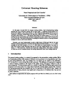
In this subsection we give some simple lower bounds for the database size and maximum time complexity of β-approximate source directed routing schemes. We first establish a lower bound for the maximum database size of β-approximate source directed routing schemes. Note that any graph with maximum degree greater than 2 has local density greater than 1.5, therefore the following lemma apply for all families F(n, D) except for F(n, 1). Lemma 3.8 Any β-approximate source directed routing scheme πSD = (USD , RSD ) for the family F(n, D) for any D ≥ 1.5 has Data(πSD ) = Ω(n). Proof: Consider the graph G shown in Figure 1. Note that G has local density 1.5 and hence G belongs to the family F(n, D) for any D ≥ 1.5. Assume without loss of generality that the identity of the bottom rightmost vertex, w, in G is 1. Given a weight assignment to the edges, a good path is a (not necessary simple) path connecting v1 and w whose weighted

15

x1

y1

x2

y2

x3

y3

x4

y4 11 00 00 00 0011 11 0011 11 00 11

v1

u1

v2

u2

v3

u3

v4

u4

w

Figure 1: The graph G length is a β-approximation to dw G (v1 , w). Upon receiving id(w) = 1, RSD (v1 ) outputs a good path. It is easy to show that for every n/2-bit binary string B there exists a weight assignment ωB to the edges of G such that (vi , ui ) is included in every good path iff the i’th bit in B is 1. Therefore RSD (v1 ) must distinguish between 2n/2 possibilities and hence Data(πSD ) = Ω(n). We now show that even on underlying graphs with constant local density, the maximum time complexity on any β-approximate source directed routing scheme is Ω(Diam). Let us note that a similar proof establishes the same result also for β-approximate point-to-point routing schemes. Lemma 3.9 Any β-approximate source directed routing scheme πSD = (USD , RSD ) for the family F(n, D) for any D ≥ 1 has Max Time(πSD ) = Ω(Diam). Proof: Let C be an n-node circle. Initially, assume all edges have weight 1. Let u and v be two vertices of distance Θ(n) on the circle. Let P be the path chosen by the router from u to v. Now, repeatedly raise the weight of the middle edge in P . At some point, P is no longer a good route from u to v, i.e., |P | ≥ β · dC (u, v). Therefore, after some topological event, a message must reach u in order to let the router choose a different path from u to v. To complete this update, Ω(Diam) time units are required.

4

The point-to-point routing scheme πP T P (β)

In this section we introduce our β-approximate point-to-point routing scheme πP T P (β) for the family F(n, D).

4.1

The update protocol UP T P (β)

The memory structure M emory(v) of each vertex v is hA(v), Aint , L(v)i. A(v) is the memory structure given to v by the source directed update protocol USD . Aint is the initial matrix 16

A(v) representing the initial graph. The component L(v) of M emory(v) is a table containing elements of the form hφ, bi, where b is a bin and φ is a token. The update protocol UP T P uses Protocol Bin0 instead of Protocol Bin. Protocol Bin0 is the same as Protocol Bin except that in step 3 we add one more substep 3.(d), described below. Substep 3.(d) of Bin0 : Each node z ∈ Q(b) adds (φ, b) to L(z).

4.2

The router protocol RP T P (β) and the data structure Data(u)

Let M be a message originated at x and destined to y. The sender x initially calculates h = dωA0 (x) (x, y), the weighted distance between x and y in A0 (x). Let q = min{βαh, n} and let l = dlog qe (i.e., 2l−1 < q ≤ 2l ). The sender then attaches the header H = (id(y), l) to the message M . Since H can be encoded with at most 2 log n bits, we obtain that the header size HD(πP T P ) is O(log n). Denote the subgraph of G induced by all vertices whose unweighted distance to y is at most 2l by Ball(H) = Γ(y, 2l ). Consider the vertices of Ball(H) as vertices of T (G) and for every node ui ∈ Ball(H), let Ri be the path from ui to r0 and let Ii be the subpath of Ri of S length 2l containing ui . Let I(Ball(H)) = i Ii . A bin b is I(Ball(H))-universal if sup(b) is outside of I(Ball(H)). In an intermediate node u along the route (including the sender x), algorithm RP T P (β) operates as follows. Upon receiving H and M emory(u) as input, RP T P (β) creates the following edge-weight matrix C(u, H) for Ball(H). Initially C(u, H) is Aint restricted to Ball(H). Now u updates C(u, H) by inspecting its table L(u). Let φ = hid(e), ω(e), ci be a token in some element (φ, b) ∈ L(u). If b is an I(Ball(H))-universal bin, φ corresponds to an event happening in Ball(H) and φ is fresh w.r.t C(u, H), then C(u, H) updates e’s entry to be (ω(e), c). After calculating C(u, H), using an algorithm similar to the Dijkstra or the Bellman-ford algorithms on the graph C(u, H), the router RP T P (β) efficiently calculates and outputs a port number connecting u to the next vertex on a simple path P (contained in Ball(H)) connecting u and y which satisfies P˜ = dωC(u,H) (u, y). The database size can be reduced further. For an intermediate node u along the route

17

from x to y, the port on which the message is to be delivered depends only on M emory(u), l and the destination y. We let Data(u) contain a table Dl for each integer l ≤ log n. Each such table contains n entries corresponding to the vertices of G. The y’s entry in Dl contains RP T P (M emory(u), id(y), 2l ). Given Data(u) and H = (id(y), l), the router RP T P outputs the port in the y’s entry in Dl . We therefore get the following lemma. Lemma 4.1 Data(πP T P (β)) = O(n log2 n).

4.3 4.3.1

Analysis Approximation and correctness

For simplicity of presentation, we first assume that the route starts at some quiet time t and that the system remains quiet during the route. We then show correctness also in the case where the route starts at a non quiet time. Fix a quiet time t. A Ball(H)-relevant event is a weight change event occurring in an edge e of Ball(H) at some time before t. A token is Ball(H)-relevant if it corresponds to a Ball(H)-relevant event. Lemma 4.2 Let b be an I(Ball(H))-universal bin. If some Ball(H)-relevant token φ was in b and b became full at time t0 ≤ t, then at time t, for any vertex u ∈ Ball(H), hφ, bi ∈ L(u). Proof: Let k be the level of b and let u ∈ Ball(H). Let ² be the event corresponding to φ and let e ∈ Ball(H) be the edge where ² occurred. Let u0 ∈ Ball(H) be the node responsible for e. Since sup(b) is outside of I(Ball(H)), we get that dT (sup(b), u0 ) ≥ 2l . Hence, by Claim 3.3, k ≥ l − 4. On the other hand dG (u0 , b) ≤ 3 · 2k+1 ≤ 6 · 2k . Therefore, dG (u, b) ≤ dG (u, u0 ) + dG (u0 , b) ≤ 2l + 6 · 2k ≤ 24 · 2k + 6 · 2k ≤ 25+k , yielding u ∈ Q(b). The lemma follows by Step 3.(d) of Protocol Bin0 and by the fact that u ∈ Q(b). Claim 4.3 For any two vertices w, z ∈ Ball(H) on the route P (x, y), at any time during the routing, C(w, H) = C(z, H). Proof: Let φ be a token that was used to update C(z, H) during the route. Since the system remains quiet during the route, by Lemma 4.2, φ was used to update C(w, H) as well. The claim follows. Lemma 4.4 The weighted length of the resulting route P (x, y) is a β-approximation of dωG (x, y, t). Proof: For a path P in Ball(H), let ωC (P ) be the weighted length of P in C(x, H). Let P 0 be a path minimizing the distance between x and y in G, i.e., at time t, ω(P 0 ) = dωG (x, y, t). Note 18

that by Lemma 3.4, P 0 is contained in Ball(H). Let P ∗ be a path from x to y contained in Ball(H) and satisfying ωC (P ∗ ) = dωC(x,H) (x, y). Consider some Ball(H)-relevant token φ. By Lemma 4.2 we get that at time t, the only Ball(H)-relevant tokens that were not used while updating C(x, h) are Ball(H)-relevant tokens that are stuck in bins of I(Ball(H)). Since each token accounts for a weight change of at most 1, by the second part of Lemma 3.4, we get that for every path P ∈ Ball(H), |ωC (P ) − ω(P )| ≤

|I(P )|δ |I(Ball(H))|δ |I(Ball(H))|(α − 1) ≤ ≤ . 3D 3D 3Dαβ

Note that all vertices of I(Ball(H)) are of unweighted distance (in G) of at most 3αβh. As G has local density at most D, |I(Ball(H))| ≤ 3βαDh. Therefore, |ωC (P ) − ω(P )| ≤ h(α − 1). By the fourth part of Lemma 3.4, h is an α-approximation to dωG (u, v, t) = ω(P 0 ), hence for all P ∈ Ball(H), |ωC (P ) − ω(P )| ≤ (α2 − α)ω(P 0 ). In particular, |ωC (P 0 ) − ω(P 0 )| ≤ · ω(P 0 ). For the same reasoning (α2 − α)ω(P 0 ). Therefore ωC (P 0 ) ≤ (α2 − α + 1)ω(P 0 ) = β+1 2 we get |ω(P ∗ ) − ωC (P ∗ )| ≤ (α2 − α)ω(P 0 ). Therefore ω(P ∗ ) ≤ (α2 −α)ω(P 0 )+ωC (P ∗ ) ≤ (α2 −α)ω(P 0 )+ωC (P 0 ) ≤ (α2 −α+

β+1 )·ω(P 0 ) ≤ βω(P 0 ). 2

If follows that ω(P 0 ) ≤ ω(P ∗ ) ≤ βω(P 0 ). By Claim 4.3, for any vertex z ∈ Ball(H), C(z, H) = C(x, H). Therefore, the resulting path Proute must satisfy ωC (Proute ) = dωC(x,H) (x, y), hence ω(P 0 ) ≤ ω(Proute ) ≤ βω(P 0 ) and the lemma follows. Let us now prove correctness also in the case where the route from x to y does not necessarily start at a quiet time. Note that also in this case, all the vertices participating in the route are in Ball(H). If at some quiet time t the message is at u and the system remains quiet during the remaining route, then by Lemmas 4.2 and 4.3, for every two vertices w and z in the remaining route from u to y, C(w, H) = C(z, H). Therefore, the path resulted from this remaining route is a path (contained in Ball(H)) connecting u and y, in particular, the message reaches y. Since we assume the system is eventually quiet for sufficiently long time period, the correctness of the scheme follows. 4.3.2

Complexities

Lemma 4.5 Avg Time(πP T P (β)) = O(D log2 n). Proof: The lemma follows from Lemma 3.6 and from the fact that the messages sent by Protocol Bin0 are the same as the messages sent by Protocol Bin. By combining Lemmas 4.1, 4.4 and 4.5, we obtain the following theorem. 19

Theorem 4.6 πP T P (β) = hUP T P , RP T P i is a β-approximate point-to-point routing scheme for the family F(n, D) with the following complexities. 1. Avg Time(πP T P (β)) = O(D log2 n). 2. Data(πP T P (β)) = O(n · log2 n). 3. HD(πP T P ) = O(log n).

References [AAPS89] Y. Afek, B. Awerbuch, S.A. Plotkin and M. Saks. Local management of a global resource in a communication network. J. ACM 43, (1996), 1–19. [AGR89]

Y. Afek, E. Gafni and M. Ricklin. Upper and lower bounds for routing schemes in dynamic networks. In Proc. 30th Symp. on Foundations of Computer Science, 1989, 370–375.

[ABLP90] B. Awerbuch, A. Bar-Noy, N. Linial and D. Peleg. Improved routing strategies with succinct tables. J. Algorithms 11, (1990), 307–341. [AP92]

B. Awerbuch and D. Peleg. Routing with polynomial communication-space trade-off. SIAM J. Discrete Math 5, (1992), 307–341.

[CCDG82] P. Chinn, J. Chavat´alov´a, A. Dewdney, and N. Gibbs. The bandwidth problem for graphs and matrices - survey. J. of Graph Theory 6, (1982), 223–254. [C01]

L. Cowen. Compact routing with minimum stretch. J. Algorithms. 38, (2001), 170–183.

[CS89]

R. F. Chung and P. D. Seymour. Graphs with small bandwidth and cutwidth. Discrete Mathematics 75, (1989), 113–119.

[DKKP95] S. Dolev, E. Kranakis, D. Krizanc and D. Peleg. Bubbles: Adaptive routing scheme for high-speed dynamic networks. SIAM J. on Comput. 29, (1999), 804–833. [EGI99]

D. Eppstein, Z. Galil and G. F. Italiano. Dynamic Graph Algorithms. In Algorithms and Theoretical Computing Handbook, M.J. Atallah, ed., CRC Press, 1999, Chapter 8.

[FG97]

P. Fraigniaud and C. Gavoille. Universal routing schemes. Distributed Computing 10, (1997), 65–78.

20

[F00]

U. Feige. Approximating the bandwidth via volume respecting embeddings. In J. of Comput. Syst. Sci., 60, (2000), 510–539.

[FT05]

U. Feige and K. Talwar. Approximating the bandwidth of caterpillars. In Proc. APPROX, LNCS 3624 Springer, 62–73, 2005.

[FK00]

J. Feigenbaum and S. Kannan. Dynamic Graph Algorithms. In Handbook of Discrete and Combinatorial Mathematics, CRC Press, 2000.

[IK00]

K. Iwama and A. Kawachi. Compact routing with stretch factor less than three. In Proc. 19th ACM Symp. on Principles of Distributed Computing, 2000, 337.

[IO03]

K. Iwama and M. Okita. Compact Routing for Flat Networks. In Proc. 17th Int. Symp. on Distributed Computing, Oct. 2003.

[KLMN04] R. Krauthgamer, J. Lee, M. Mendel, and A. Naor. Measured descent: A new embedding method for finite metrices. In Proc. 45th IEEE Symp. on Foundations of Computer Science, Oct. 2004. [K05]

A. Korman. General Compact Labeling Schemes for Dynamic Trees. In Proc. 19th Int. Symp. on Distributed Computing, Sep. 2005.

[KPR04]

A. Korman, D. Peleg and Y. Rodeh. Labeling schemes for dynamic tree networks. Theory of Computing Systems 37, (2004), 49–75.

[KP03]

A. Korman and D. Peleg. Labeling schemes for weighted dynamic trees. In Proc. 30th Int. Colloq. on Automata, Languages and Prog., July 2003, 369–383.

[L92]

N. Linial. Locality in distributed graph algorithms. SIAM J. on Computing 21, (1992), 193–201.

[P00]

D. Peleg. Distributed computing: A Locality-Sensitive Approach. SIAM, 2000.

[PU89]

D. Peleg and E. Upfal. A tradeoff between size and efficiency for routing tables. J. ACM 36, (1989), 510–530.

[SK85]

N. Santoro and R. Khatib. Labeling and implicit routing in networks. The Computer Journal 28, (1985), 5–8.

[TZ01]

M. Thorup and U. Zwick. Compact routing schemes. In Proc. 13th ACM Symp. on Parallel Algorithms and Architectures, July 2001, 1–10.

21