Dynamic Speech Emotion Recognition with State-Space Models

23rd European Signal Processing Conference (EUSIPCO)

DYNAMIC SPEECH EMOTION RECOGNITION WITH STATE-SPACE MODELS Konstantin Markov∗ , Tomoko Matsui† , Francois Septier‡ , Gareth Peters§ ∗

The University of Aizu, Japan

†

Institute of Statistical Mathematics, Japan

ABSTRACT Automatic emotion recognition from speech has been focused mainly on identifying categorical or static affect states, but the spectrum of human emotion is continuous and time-varying. In this paper, we present a recognition system for dynamic speech emotion based on state-space models (SSMs). The prediction of the unknown emotion trajectory in the affect space spanned by Arousal, Valence, and Dominance (A-V-D) descriptors is cast as a time series filtering task. The statespace models we investigated include a standard linear model (Kalman filter) as well as novel non-linear, non-parametric Gaussian Processes (GP) based SSM. We use the AVEC 2014 database for evaluation, which provides ground truth A-V-D labels which allows state and measurement functions to be learned separately simplifying the model training. For the filtering with GP SSM, we used two approximation methods: a recently proposed analytic method and Particle filter. All models were evaluated in terms of average Pearson correlation R and root mean square error (RMSE). The results show that using the same feature vectors, the GP SSMs achieve twice higher correlation and twice smaller RMSE than a Kalman filter. Index Terms— Emotion recognition, Affect recognition, Kalman filter, Gaussian Process state-space model 1. INTRODUCTION Automatic recognition of human emotions expressed by speech or body language is an important task since it can not only facilitate development of new human centric applications, but also help diagnose and prevent mental health disorders such as depression which exhibit specific emotional patterns. Most of the research on speech emotion recognition in recent years has been focused on categorical emotion classification. Categories such as happiness anger, and fear are commonly used to label speech utterances and build classifiers. Another way of representing emotions is by the affect space. This space usually has two or three dimensions named Arousal, Valence, and Dominance. A point in this space represents a particular emotion. Emotions varying in time form a trajectory in it. The task of dynamic emotion recognition is to infer this trajectory from the speech signal.

978-0-9928626-3-3/15/$31.00 ©2015 IEEE

2122

‡

Telecom Lille, CRIStAL, France

§

University College London, UK

There are just a few studies on this task one of which is the study of Wollmer et al. [1]. It uses long-short term RNN to capture the time dependencies in emotion trajectories. Recently, a series of annual Audio-Visual Emotion Challenge (AVEC) and workshops has been under way, which has advanced the research in this area by providing common benchmark test sets. Some of the techniques presented at these workshops include multi-stage approach based on hidden Markov models [2], multi-scale dynamic cues [3], and Partial Least Square Regression [4]. Our approach is to consider emotion trajectories as time series and apply methods from time series analysis. One widely used method is Bayesian filtering based on statespace models (SSMs). A classical example is the Kalman filter [5]. It has been successfully used for temporal music emotion recognition [6]. However, the Kalman filter is a linear system and has its limitations. There exist non-linear SSMs such as the Extended Kalman filter (EKF) and Unscented Kalman filter (UKF), but they put certain constraints on the SSM state and measurement functions. A better solution is to use Gaussian Processes (GPs) which are non-linear, non-parametric models [7]. They have been successfully applied in various tasks including speech and music processing [8–10]. Previously, we have also used GPs for static music emotion recognition [11]. A number of GP based state-space models (GP-SSM) have been proposed recently. GP-BayesFilters [12] use GPs as non-linear functions and derive GP-Particle filter, GP-EKF, and GP-UKF algorithms using Monte Carlo sampling. In [13, 14], an analytic filtering approximation algorithm is presented, but lacks an analytic approach to GP-SSM parameter learning. An attempt to derive such an algorithm is done in [15], which, however, has some stability problems. A Particle Markov Chain Monte Carlo (PMCMC) training method is described in [16], but the MC based learning is notoriously slow. In this study, we use the AVEC 2014 database [17] which provides ground truth labels for the A-V-D affect vectors and this makes possible to train the state and measurement GP functions of the state-space model independently. For the filtering with GP-SSMs we adopted the analytic algorithm from [14] as well as a GP Particle filter algorithm similar to the one in [12].


2. STATE-SPACE MODELS

3. KALMAN FILTER

We consider state-space models defined by xt yt

= =

f (xt−1 ) + ut , g(xt ) + vt

d

(1)

e

(2)

xt ∈ R , yt ∈ R ,

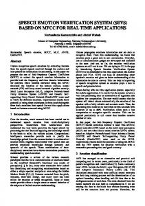
where f () and g() are unknown functions governing temporal state dynamics and state-to-measurement mapping respectively. System and observation noises, ut ∼ N (0, Σu ) and vt ∼ N (0, Σv ), are both Gaussian with uncorrelated dimensions. Figure 1 shows the SSM as a graphical model with probabilistic dependencies between variables. The initial state x0 is assumed to have known Gaussian distribution p(x0 ) = N (µx0 , Σx0 ). For a sequence of T measurements, the tasks of filtering and smoothing are to find approximations to the posterior distributions p(xt |y1:t ) and p(xt |y1:T ), t = 1, . . . , T . When these approximations are given by Gaussian distributions the corresponding models are referred to as Gaussian filters or smoothers. In this case, as shown in [18], the filtering distribution can be approximated as N (xt |µxt , Σxt ),

p(xt |y1:t ) ≈ µxt Σxt x

(3)

x

=

y −1 (yt − µyt ), (4) µt pred + Σx,y t (Σt )

=

y −1 T (Σx,y Σt pred − Σx,y t (Σt ) t ) .

x

(5)

x

where µt pred and Σt pred are the parameters of the Gaussian approximation to the predictive distribution p(xt |y1:t−1 ) ≈ x x N (xt |µt pred , Σt pred ). Generally, the means and covariance matrices required in Eqs. (4) and (5) cannot be computed analytically except when f () and g() are linear as in the Kalman filter case.

Fig. 1. Graphical representation of a state-space model. States xt are continuous latent variables and measurements yt are observable vectors. Arrows show the probabilistic relationship between variables.

When we apply a SSM for continuous speech emotion recognition, states xt would represent the unknown affect vector, i.e., Arousal-Valence-Dominance values, and yt would correspond to feature vectors extracted from the speech signal. When observations of the state variable are available during training, f () and g() can be learned independently which makes the SSM parameter estimation simpler.

2123

As mentioned above, when state dynamics and measurement functions are linear, such as f (x) = F x and g(x) = Gx with matrix parameters F and G, an analytic solution can be easily obtained. The means and covariances from Eqs.(4) and (5) are computed as x

µt pred x Σt pred µyt Σyt Σx,y t

= F µxt−1 , = = = =

F Σxt−1 F T + Σu , x Gµt pred , x GΣt pred GT + Σv , x Σt pred GT .

(6) (7) (8) (9) (10)

In general, when there are no ground truth observations of the latent state variables, estimation of F and G as well as the noise variances Σu and Σv can be done using likelihood maximization via expectation-maximization algorithm [5]. However, when they are available, simple multivariate linear regression can be used to obtain the necessary estimates. 4. GAUSSIAN PROCESSES SSM Having non-linear functions f () and g() would greatly increase the expressiveness of the state-space model, but introduces two problems - what kind of non-linearity is suitable for the task at hand and how to estimate the parameters. Gaussian Processes allow eliminating the first problem and, when state observations are available, provide solution to the second. In GP inference, the non-linear function is marginalized out and there is no need to define it. The GP kernel function parameters can be learned using approximations and gradient descent methods [7]. However, filtering with SSM when f () and g() are described by GPs is not straightforward. There are just a few studies on this problem and no common and efficient algorithm exists yet. In our experiments, we adopted the solution recently proposed in [14]. It is based on analytic moment matching to derive Gaussian approximation to the filtering distribution. In addition, we implemented a Particle filter based approximation similar to the one proposed in [12]. 4.1. Gaussian Process Regression Given input training data vectors X = {xi }, i = i, . . . , n and their corresponding target values z = {zi }, a general regression model relates them as: zi = f (xi ) + i , where t ∼ N (0, σ 2 ) and f () is an unknown non-linear function. In GP, it is assumed that this function is normally distributed, i.e. the vector f = [f (x1 ), . . . , f (xn )] has Gaussian distribution f ∼ N (m, K), where K = {kij = k(xi , xj )} is a kernel covariance matrix and the mean m is often set to zero. This assumption allows expressing in closed form the predictive


distribution of a test target z∗ only in terms of training data and the input vector x∗ : = N (z∗ |m∗ , σ∗2 ),

p(z∗ |x∗ , z, X)

(11)

m∗

= k∗T (K + σn2 I)−1 z,

σ∗2

= k(x∗ , x∗ ) − k∗T (K + σ 2 I)−1 k∗

where k∗ = k(x∗ , xi ), i = i, . . . , n. The computational complexity of this operation is O(n2 ). Covariance kernel parameters are learned by maximizing R the marginal likelihood p(z|X, θ) = p(z|f )p(f |X, θ)dθ w.r.t. θ which is known as maximum likelihood type II approximation. 4.2. GP-SSM analytic filter States xt and observations yt of the GP-SSM are multidimensional vectors, but the GP regression targets, as described in Section 4.1, are scalars. A simple way to overcome this discrepancy is to assume that the target dimensions are independent given a test input and train a separate GP for each dimension. Analytic approximations to the means and variances from Eqs.(4) and (5) have been proposed in [13] and [14]. For example, the mean of the predictive distribution for target dimension k is calculated as1 x

(µt pred )k x qk,i

=

(βkx )T qkx ,

=

αf2k |Σxt−1 Λ−1 k

(12) − 12

approach is the selection of the so-called proposal distribution which should approximate the importance distribution π(xt |xt−1 , y1:t ). Often, the proposal distribution is set to p(xt |xt−1 ) which can be evaluated using the GP state model. Algorithm 1 provides the steps of the GP Particle filter. The number of particles is set to N . It is assumed that GP parameters θx and θy for each target dimension are already obtained. Algorithm 1 GP Particle filter ˆ 1:T Input: N, T, y1:T , θx , θy , µx0 , Σx0 , Output: x 1. for i = 1, . . . , N 2. xi0 ∼ N (µx0 , Σx0 ) ⇒ initialize particle i 3. w0i = 1/N ⇒ initialize weight i 4. end 5. for t = 1, . . . , T 6. Resample particles xit according to weights wti 7. for i = 1, . . . , N 8. fti , Σix,t = GP (xit−1 |θx ) 9. xit ∼ N (fti , Σix,t + Σu ) ⇒ propagate particle i 10. gti , Σiy,t = GP (xit |θy ) 11. wti = N (yt |gti , Σiy,t + Σv ) ⇒ update weight i 12. end P 13. wti = P wti / i wti ⇒ normalize weights ˆ t = i wti xit ⇒ estimated mean of p(xt |y1:t ) 14. x 15. end ˆ 1:T 16. return x

+ I|

1 exp(− (xi − µxt−1 )T 2 (Σxt−1 + Λk )−1 ((xi − µxt−1 )),

5. EXPERIMENTS

i = 1, . . . , n, where Λ = diag[l12 , . . . , ld2 ] is a diagonal matrix with the length-scales of the squared exponential kernel function 1 kSE (xi , xj ) = α2 exp(− (xi −xj )T Λ−1 (xi −xj )), (13) 2 which represents the “distance” between a pair of vectors xi and xj . The other kernel parameter, α2 , is called the function variance. 4.3. GP Particle filter In contrast to the analytic method from the previous section, particle filtering approximates the distribution of interest using the sequential importance re-sampling (SIR) Monte Carlo method [19]. This method is often used in SSM when distributions p(xt |xt−1 ) and p(yt |xt ) are unknown, but probabilities can be evaluated. Central to particle filtering 1 In order to save space, we do not provide all the expressions for Eqs.(4) and (5).

2124

For our experiments we developed speech emotion recognition systems based on three SSM: Kalman filter, GP-SSM filter and GP Particle filter. In addition, we implemented the corresponding smoothing algorithms: RTS smoother, GPSSM smoother and GP Particle smoother. The main algorithmic difference between filtering and smoothing is an additional backward sweep over the filter output. Each system is evaluated in terms of average Pearson correlation coefficient R between each of the reference A, V, or D sequences and its corresponding prediction averaged over all test utterances. We have to note that for many test samples, the correlation coefficient showed negative values resulting in reduced total average 2 . In addition to R, the root mean square error (RMSE) is also used as an evaluation measure. In all cases, for GP parameter training and inference we used the GPML toolbox [20]. 2 Averaged results in the next sections are not directly comparable with the official AVEC 2014 results because the AVEC scoring technique uses the absolute R value. This increases the average to the 0.5-0.6 range. We, however, believe that this approach masks system errors which are the reason for negative R values.


5.1. Database and feature extraction The database we used in our experiments has been released as part of The Audio/Visual Emotion Challenge and Workshop (AVEC 2014) [17]. It consists of recordings from 84 subjects. There are 100 recordings for training and as many for testing. Duration ranges from 6 to 248 seconds. Each recording is annotated using three affective dimensions: Arousal, Valence, and Dominance (A-V-D) which form a basis for emotion analysis in psychology. The AVEC 2014 database includes speech features extracted using the openSMILE toolkit [21]. The feature set consists of 32 energy and spectral related low level descriptors (LLD) and 6 voicing related LLDs. These features are aggregated in windows of 3 seconds with 1 second overlap and various statistics such as mean, standard deviation, flatness, skewness, kurtosis, and functionals such as regression coefficients, local minima/maxima, etc., are calculated for each window resulting in a 2268 dimensional feature vector. Since the feature dimension is too high for the GP based SSMs, we used several feature subsets. The first one, called means1, includes only the LLD means. In the second one, means2, we included means of LLD delta coefficients (∆LLDs) as well. Next, we added the standard deviation of LLDs and ∆LLDs and call this set stat1. Finally, we selected all statistical functionals for LLDs and ∆LLDs into a set named stat2. 5.2. Kalman filter results

Feature set # dims

means1 means2 stat1 stat2 all

38 76 152 456 2268

Feature set

Filter

Name

# dims

means1 means2 stat1

38 76 152

Filter

R

RMSE

R

RMSE

0.0850 0.0896 0.1096

0.0661 0.1758 0.1779

0.0880 0.0919 0.1108

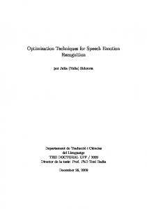
Table 2. GP-SSM filter and GP-SSM smoother results.

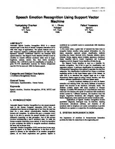
5.4. GP Particle filter results With the GP Particle filter and smoother based systems, in addition to the squared exponential kernel, Eq.(13), we used linear kernel kl (xi , xj ) = (xTi xj + 1)/l as well. Here l is a length parameter. Table 3 summarizes the results for the means1 and means2 feature sets. Unfortunately, for other feature sets evaluation time was unreasonably long. In all cases, we used 5000 particles for filtering and 500 for smoothing. As these results show, GP Particle filter and smoother perform similarly to the GP-SSM, especially when squared exponential kernel is used. The linear kernel is little bit worse in terms of R, but still better than the Kalman filter. In terms of RMSE, however, their performances are comparable.

RMSE

R

RMSE

0.0350 0.0881 0.0987 0.1430 0.1725

0.1598 0.1691 0.1802 0.2057 0.2249

0.0405 0.0960 0.1112 0.1575 0.1591

0.1668 0.1763 0.1862 0.2059 0.1970

Name

Filter

# dims

R

Smoother

RMSE

R

RMSE

0.1406 0.1598

0.1403 0.1525

Linear covariance function means1 means2

38 76

0.1219 0.1631

0.1303 0.1430

Squared Exponential covariance function means1 means2

Smoother

R

Smoother

0.1445 0.1895 0.1769

Feature set

The Kalman filter based speech emotion recognition system was evaluated using all feature sets and Table 1 summarizes its performance together with the one using a linear RauchTung-Striebel (RTS) smoother. Results clearly show that an increased feature vectors dimension improves the correlation coefficient R, but also worsens the root mean square error.

Name

vectors, the GP-SSM systems achieved results better than the best of the linear SSMs in Table 1. For the same feature sets, correlation R is two or more times higher and the RMSE is about two times smaller.

38 76

0.1417 0.1642

0.0850 0.0890

0.1257 0.1603

0.0742 0.0897

Table 3. GP Particle filter and GP Particle smoother results.

6. CONCLUSION

Table 1. Kalman filter and linear RTS smoother results.

5.3. GP-SSM filter results Table 2 shows the performance of the GP-SSM filter and GP-SSM smoother based systems. Results are shown only for means1, means2, and stat1 feature sets, because the other two sets’ dimensionality imposed prohibitive memory requirements. Nevertheless, even with much smaller feature

2125

We have developed and investigated a dynamic speech emotion recognition system using two different state-space models such as linear Kalman filter and a novel non-linear, nonparametric Gaussian Processes-based SSM. Kalman filters are widely used and well known SSM. On the other hand, the GP based models are new and there are few studies focusing on learning and inference algorithms for them. We were able to simplify the GP-SSM learning by utilizing the AVEC 2014 database which provides ground truth labels for the latent affect states. For the filtering and smoothing, however, there is no common and efficient algorithm. We compared the performance of a recently proposed analytic approximation


based algorithm and a GP based Particle filter in terms of Pearson correlation coefficient and root mean square error with respect to the conventional Kalman filter. Both GP filtering algorithms showed about two times better results when the same feature vectors are used. A disadvantage of the GP-SSMs, however, is their memory and computational complexity which is much higher. REFERENCES [1] M. Wollmer, F. Eyben, S. Reiter, B. Schuller, C. Cox, E. Douglas-Cowie, and R. Cowie, “Abandoning emotion classes - towards continuous emotion recognition with modelling of long-range dependencies,” in Proc. INTERSPEECH, 2008, vol. 2008, pp. 597–600. [2] Hongying Meng and Nadia Bianchi-Berthouze, “Naturalistic affective expression classification by a multistage approach based on hidden markov models,” in Affective computing and intelligent interaction, pp. 378– 387. Springer, 2011. [3] Jérémie Nicolle, Vincent Rapp, Kévin Bailly, Lionel Prevost, and Mohamed Chetouani, “Robust continuous prediction of human emotions using multiscale dynamic cues,” in Proceedings of the 14th ACM international conference on Multimodal interaction. ACM, 2012, pp. 501–508. [4] Hongying Meng, Di Huang, Heng Wang, Hongyu Yang, Mohammed AI-Shuraifi, and Yunhong Wang, “Depression recognition based on dynamic facial and vocal expression features using partial least square regression,” in Proceedings of the 3rd ACM International Workshop on Audio/Visual Emotion Challenge, New York, NY, USA, 2013, AVEC ’13, pp. 21–30, ACM. [5] Simon Haykin, Ed., Kalman filtering and neural networks, John Wiley & Sons, 2001. [6] E.M. Schmidt and Y.E. Kim, “Prediction of timevarying musical mood distributions using kalman filtering,” in Machine Learning and Applications (ICMLA), 2010 Ninth International Conference on, Dec 2010, pp. 655–660. [7] C. Rasmussen and C. Williams, Gaussian Processes for Machine Learning, Adaptive Computation and Machine Learning. The MIT Press, Cambridge, Massachusetts, 2006. [8] G. Henter, M. Frean, and W. Kleijn, “Gaussian process dynamical models for nonparametric speech representation and synthesis,” in Proc. IEEE International Conference on Acoustics, Speech and Signal Processing (ICASSP), 2012, pp. 4505–4508. [9] H. Park, S. Yun, S. Park, J. Kim, and C. Yoo, “Phoneme classification using constrained variational Gaussian process dynamical system,” in Advances in Neural

2126

Information Processing Systems 25, 2012, pp. 2015– 2023. [10] J. Wang, D. Fleet, and A. Hertzmann, “Gaussian process dynamical models for human motion,” IEEE Transactions on Pattern Analysis and Machine Intelligence, vol. 30, no. 2, pp. 283–298, 2008. [11] K. Markov and T. Matsui, “Music genre and emotion recognition using Gaussian processes,” IEEE Access, vol. 2, pp. 688–697, 2014. [12] J. Ko and D. Fox, “GP-BayesFilters: Bayesian filtering using Gaussian process prediction and observation models,” Autonomous Robots, vol. 27, no. 1, pp. 75–90, 2009. [13] M. Deisenroth, M. Huber, and U. Hanebeck, “Analytic moment-based Gaussian process filtering,” in Proc. 26th Annual International Conference on Machine Learning, 2009, ICML ’09, pp. 225–232. [14] M. Deisenroth, R. Turner, M. Huber, U. Hanebeck, and C. Rasmussen, “Robust filtering and smoothing with Gaussian processes,” IEEE Transactions on Automatic Control, vol. 57, no. 7, pp. 1865–1871, 2012. [15] R. Turner, M. Deisenroth, and C. Rasmussen, “Statespace inference and learning with Gaussian processes,” in Proc. 13th Internatioanl Conference on Artificial Intelligence and Statistics (AISTATS), 2010, pp. 868–875. [16] R. Frigola, F. Lindsten, T. Schon, and C. Rasmussen, “Bayesian inference and learning in Gaussian process state-space models with particle MCMC,” in Advances in Neural Information Processing Systems, 2013, pp. 3156–3164. [17] M. Valstar, B. Schuller, K. Smith, T. Almaev, F. Eyben, J. Krajewski, R. Cowie, and M. Pantic, “AVEC 2014 – 3D dimensional affect and depression recognition challenge,” in Proc. 4th ACM international workshop on Audio/visual emotion challenge, 2014. [18] M. Deisenroth and H. Ohlsson, “A general perspective on Gaussian filtering and smoothing: Explaining current and deriving new algorithms,” in IEEE American Control Conference (ACC), 2011, 2011, pp. 1807– 1812. [19] A. Doucet, N. De Freitas, and N. Gordon, Sequential Monte Carlo methods in practice, Springer, 2001. [20] C. Rasmussen and H. Nickisch, “Gaussian processes for machine learning (GPML) toolbox,” Journal of Machine Learning Research, vol. 11, pp. 3011–3015, 2010. [21] F. Eyben, M. Wöllmer, and B. Schuller, “Opensmile: the munich versatile and fast open-source audio feature extractor,” in Proceedings of the international conference on Multimedia. ACM, 2010, pp. 1459–1462.