Abstract— We present the real-world test of the SPECIALIST algorithm in which dynamic speed limits were used to resolve shock waves on freeways.
2010 13th International IEEE Annual Conference on Intelligent Transportation Systems Madeira Island, Portugal, September 19-22, 2010
MB8.6
Dynamic speed limit control to resolve shock waves on freeways – Field test results of the SPECIALIST algorithm A. Hegyi, S.P. Hoogendoorn Abstract— We present the real-world test of the SPECIALIST algorithm in which dynamic speed limits were used to resolve shock waves on freeways. The real-world test was performed in the period September 2009–February 2010 on a 14 km long stretch on the Dutch A12 freeway. For the evaluation of the algorithm various performance measures were determined for each activation of the speed limits. The results show that the SPECIALIST algorithm can resolve shock waves in nearly 80% of the cases when the algorithm activated for shock waves. However, in approximately 50% of the activations the algorithm activated for jam types other than shock waves, in which case the effectivity was 40– 50%. Due to the tuning the stability of the traffic flow could be significantly improved, and the number of average activations per day was increased from 1.5 to 2.9 activations per day. The SPECIALIST algorithm was not only evaluated for traffic performance, but also for the correctness of the algorithm for real traffic in terms of expected qualitative behavior. Although the general operation of the algorithm is according to the theoretical expectations, some points for further improvements are identified during the test.
I. INTRODUCTION In earlier publications we presented an approach to dynamic speed limit control to eliminate shock waves on freeways that is based on shock wave theory, the so-called SPECIALIST algorithm (SPEed ControllIng ALgorIthm using Shock wave Theory) [1], [2]. It was shown by simulation that the algorithm is capable of resolving shock waves, and that the improvement of the total time was that the vehicles spend on the freeway is comparable with approaches using other control techniques [3], [4]. On freeways basically two types of traffic jams can occur: jams with the head fixed at a bottleneck location and jams that have an upstream moving head and tail. Here we focus on the second type, which are often called shock waves [3] or wide moving jams [5]. We will use the term shock wave for these jams. These jams are typically short jams (say, 1-2 km) that propagate upstream, due to the incoming vehicles at their tail and the leaving vehicles at their head. They can remain existent for a long time and distance [5]. Consequently, every vehicle that enters the freeway upstream of the jammed area will have to pass through the jammed area, which increases travel times, creates potentially unsafe situations, and increases noise and air pollution by braking and accelerating vehicles. Shock waves typically have a significantly lower outflow than the capacity of the freeway, which motivates the idea that traffic flow can be improved by A. Hegyi and S.P. Hoogendoorn are with the Department of Transport & Planning, Fac. CiTG, TU Delft, P.O. Box 5048, 2600 GA Delft, The Netherlands. {a.hegyi, s.p.hoogendoorn}@tudelft.nl.
978-1-4244-7658-9/10/$26.00 ©2010 IEEE
resolving shock waves. The difference between the free flow capacity and the queue discharge rate is around 30% [5]. In the literature two main approaches can be found to dynamic speed limit control aiming at flow improvement. The first emphasizes the homogenization effect [6]–[9], whereas the second is focused on preventing traffic breakdown or resolving existing jams by reducing the flow by means of speed limits [3], [4], [10], [11].The basic assumption of homogenization is that speed limits can reduce the speed (and/or density) differences, by which a more stable (and safer) flow can be achieved. The flow reduction approach focuses more on preventing or resolving too high densities (including jams) by limiting the inflow to them. By resolving the jams (the bottlenecks), higher flows can be achieved in contrast to the homogenization approach as demonstrated in [3], [4], [10]. SPECIALIST is of the flow limitation type, is based on a simple principle, has a very low computational demand, and has tuning parameters that have a physical interpretation which makes the tuning parameters straightforward. In the remainder of the paper the theory of the algorithm will be discussed in Section II. The algorithm that was developed and tested based on this theory is presented in Section III. Section IV discusses the tuning variables and the approach to the tuning procedure. The approach for the evaluation of the performance of the algorithm is discussed in Section V, followed by the description of the implementation set-up in Section VI. In Section VII the results are discussed, and the conclusions are presented in Section VIII. II. THEORY OF SPECIALIST The theory of resolving shock waves by dynamic speed limits is based on the shock wave theory as also applied by Lighthill and Whitham in their famous paper [12]. Before explaining the approach for shock wave resolution we explain one of the fundamental relationships in shock wave theory. Although shock wave theory goes further than what is presented here, we only present one fundamental aspect, which is necessary to understand the remainder of the paper. A. Shock wave theory One of the basic relationships in shock wave theory is the relationship between the time-space graph of the traffic states (as shown on the left in Fig. 1) and the densityflow graph (as shown on the right in Fig. 1). The timespace graph shows the traffic states on a road stretch (along the vertical axis) and their propagation over time (in the horizontal direction). In the figure a short traffic jam is shown 519
12
3500
8 2
6 4
1
10 B
2500 2000 1500
2
500 0.2
0.4 time (h)
0.6
0 0
3000
4 C D
5
3
6 6
E
4
100 150 density (veh/km)
0 0
200
Fig. 1. According to the shock wave theory the propagation of the front between two traffic states in the left figure has the same slope as the line connecting the two states in the density-flow diagram in the right figure. The arrow indicates the travel direction.
that propagates upstream (area 2) and which is surrounded by traffic in free-flow (areas 1). The density-flow diagram shows the corresponding density and flow values for these states. Shock wave theory states that the front (boundary) between two states in the left figure has the same slope as the slope of the line that connects the two states in the right figure. Note that the slopes in both figures have the unit of km/h, and that states in the right figure correspond to areas in the left figure. The orange lines (light gray in black and white) indicate the fundamental diagram (as a reference). The importance of this relationship is that if the different traffic states on a freeway stretch are known, then their future evolution can be predicted by describing the fronts between them. This basic relationship will be used in the theory for resolving shock waves. B. Control approach The approach to resolve shock waves consists of four phases and starts with a shock wave similar to the example above. Phase I. Assume a shock wave (as shown in Fig. 2) is detected on the freeway. (How the shock wave is detected will be explained in Section III.) We assume that the traffic state upstream (state 6) and downstream (state 1) of the shock wave is in free flow which is generally the case in real traffic. In Fig. 2 the phases are indicated at the top of the left subfigure. For the sake of readability of the figures we assume that state 1 and state 6 are equal, but the theory also holds for the case when they are unequal. Phase II. As soon as the shock wave is detected the speed limits upstream of the shock wave are switched on. This leads to a state change in the speed-controlled area from state 6 to state 3 (in Fig. 2 approximately from 4-8 km), and to the boundary between areas 6 and 3. State 3 has the same density as state 6, as the density does not change when the speed limits are lowered on a longer stretch: no vehicles can suddenly appear or disappear. However, the flow of state 3 is lower than that of state 6 due to the combination of the same density with a lower speed. As shown by the density-flow graph, the front between states 2 and 3 will propagate backwards with a lower speed than the front between states 1 and 2, and consequently the
0.2
0.4 time (h)
2500 2000 1500
3
1000
6
2
2
500
F
50
1,6
2
8
4
1000
2 0 0
1 location (km)
flow (veh/h)
location (km)
3000
1
5
3500
1
A
10
4000
Phase II Phase IV Phase I Phase III
flow (veh/h)
4000 12
0.6
0 0
50
100 150 density (veh/km)
200
Fig. 2. The four phases of the SPECIALIST algorithm. Phase I: The shock wave is detected. Phase II: Speed limits are turned on in areas 2, 3, and 4. The shock wave dissolves. Phase III: The speed-limited area (area 4) resolves and flows out efficiently. Phase IV: The remaining area 5 is a forward propagating high-speed high-flow wave.
two will intersect and the shock wave will be resolved after some time. At the upstream end of the speed-limited area traffic will flow into this area, with the speed equaling the speed limit and with a density that is in accordance with the speed, typically significantly higher than the density of state 3 (which was the density corresponding to free-flow). This state is called state 4. The front between states 6 and 4 will propagate upstream or downstream depending on the flow of state 4. (The density and consequently the flow is a tuning variable, which will be explained in Section IV.) We choose the initial length of the speed-limited stretch such that the creation of state 3 exactly resolves the shock wave. This length can be determined by using point D (the intersection of the fronts 1-2 and 2-3) and the known slope of front 3-4. The length of the stretch CE depends on the density and flow associated with states 1, 2 and 6, the speed corresponding to state 3 (and consequently, the resulting flow reduction), and the physical length of the detected jam. Phase III. When the shock wave (area 2) is resolved, there remains an area with the speed limits active (state 4) with a moderate density (higher than in free-flow, but lower than in a shock wave) and a moderate speed. A basic assumption in this theory is that the traffic from such an area can flow out more efficiently than a queue discharging from full congestion as in the shock wave. So, the traffic leaving area 4 will have a higher flow and a higher speed than state 4, represented by state 5. This leads to a backward propagating front between states 4 and 5, which resolves state 4. Phase IV. What remains is state 5, and state 6 upstream and state 1 downstream of it. The fronts between states 1 and 5, and between states 6 and 5 propagate downstream, which means that eventually the backward propagating shock wave is converted into a forward propagating wave leading to a higher outflow of the link as shown in Fig. 2. Obviously, not all traffic situations are suitable to construct the above control scheme. The exact requirements for such a scheme will be discussed in Section III-C when the resolvability assessment is discussed.
520
III. ALGORITHM DEVELOPMENT Based on the theory in Section II an algorithm is developed that is suited for real-world implementation. The algorithm consists of four steps: shock wave detection, control scheme generation, resolvability assessment, and control scheme application, which will be detailed in the following sections. A. Shock wave detection In the shock wave detection step the shock wave is detected by using thresholds vmax (km/h) for the speed and qmax (veh/h) for the flow measurements, by assuming that in segment i, a shock wave is present if qi ≤ qmax and vi ≤ vmax . When there are no other types of jams on the considered stretch, this identifies the location of the shock wave. To compensate for the dependency of the head and tail location on the threshold values, and to cope with the fact that the shock wave can only be detected at discrete locations and discrete times additional offsets xhead-offset (km) and xtail-offset (km) are defined for the estimation of the location of the head and tail. The location of the shock wave head and the tail that the algorithm uses to determine the control scheme is the sum of the detector locations corresponding to the jam and the offsets. In this way even when the jam is detected by only one detector, the jam length will larger than zero. B. Control scheme generation In this step all the traffic states in the control scheme are determined. The traffic states are denoted v[j] , q[j] , ρ[j] , j ∈ {1, . . . , 6} for the six states. Since q[j] = ρ[j] v[j] , it is sufficient to determine two of the three variables for each state. The areas directly upstream and downstream of the shock wave that are not falling below the thresholds qmax and vmax are classified as free-flow, and the measurements from these areas are determined to calculate the average states upstream and downstream of the shock wave. The average flow q[6] and q[1] (veh/h/lane) and average density ρ[6] and ρ[1] (veh/km/lane) respectivelyPupstream and downstream are determined by q[6] = (1/N ) i∈I[6] qi , P and ρ[6] = (1/N ) i∈I[6] (qi /vi ), (and similarly for state 1) where qi (veh/h/lane) and vi (km/h) are respectively the flow and speed measurements of segment i, and I[6] and I[1] is the set segment indexes of the segments in free flow respectively upstream and downstream from the jam, and N the number of segments considered. This determines states 1 and 6. The density of state 2 is determined in a different way since typically a very low speed is associated with state 2 and induction loop detectors are known to be inaccurate for low speeds. The density of state 2 is determined by using the density and flow of state 1, the flow of state 2, and solving v[1,2] = (q[1] −q[2] )/(ρ[1] −ρ[2] ), for ρ[2] , where v[1,2] denotes the propagation speed of the head of the shock wave. The propagation speed of the head of the shock wave can be taken from off-line data, since it is well-known to be fairly constant (around -18 km/h). State 3 directly follows from the density of state 6 and the used speed reduction. The speed of state 4 equals the value of the speed limits. However, the
density of state 4, and the density and flow of state 5 do not follow from the shock wave theory and can be considered as a design variables for which heuristic tuning rules can be given. For now, it is sufficient to assume that they have a fixed value. Tuning will be discussed in Section IV. When all six states are determined, the control scheme can be constructed. This involves the determination of the various fronts and their intersection points by solving straightforward linear equations based on the traffic states and shock wave theory. Due to space limitations we do not present the equations here. C. Resolvability assessment After the construction of the control scheme the resolvability is assessed. A shock wave is as resolvable if: 1) The control scheme can be constructed given the measured and calculated traffic states 1–6. This means that the head and tail of area 2 should converge, otherwise the shock wave will not be resolved. The same applies for area 4. 2) State 5 should has higher flow and a higher density than state 1, otherwise there is no forward propagating front between these two states. Furthermore, the speed of state 5 should be less than or equal to the speed of state 1 in order to preserve the general shape of the fundamental diagram in free flow. 3) The speed in area 6 is higher than the speed limit, otherwise the speed limits do not have any effect. 4) The necessary length of the speed-limited stretch is smaller than the available upstream free-flow area. If these conditions are satisfied, the shock wave is classified as resolvable and the control scheme is applied. Otherwise, the algorithm waits for new data. D. Control scheme application If the control scheme is determined and the shock wave is resolvable then the speed limit can be activated. For each gantry location it is determined at what time it falls in the area’s 2, 3, or 4 (where the speed limit should be active). IV. TUNING In the algorithm there are nine parameters that can be selected by the designer of the control system. For these variables heuristic tuning rules can be given, partially based on offline traffic date and partially based on the on-line (closed-loop) behavior of the algorithm. Below we discuss the tuning approach for these variables. The actual changes that were made to tune the parameters will be discussed in Section VII together with the results. Due to spacial limitation we only discuss the parameters here that were changed during the test. One of the most important tuning parameters is the density associated with state 4. The speed of state 4 is determined by the speed limits, however the choice of the density is a design variable that influences the shape of the control scheme. If the density is chosen higher, the slope between states 4 and 6 will be less steep, which means that the tail of
521
speed limits (km/h)
the speed limits will propagate less quickly backwards. This relationship also can be understood the other way around: by letting the tail of the speed limits (the front between states 4 and 6) propagate faster backwards, the density in area 4 can be kept low. The relevance of the density is that traffic traveling at a given speed is stable at sufficiently low densities and becomes more and more unstable with increasing densities. By selecting 4 properly (low enough), the stability of the traffic under the speed limits can be ensured. Other tuning parameters are the speed v[5] , and flow q[5] of state 5. These parameters determine the slopes 1–5, 4– 5 and 5–6. Slope 4–5 determines how the speed limits are release at the head of the speed-limited area. By changing the speed of the slope the flow of state 5 can be influenced. Obviously, the resulting flow cannot take any value, due to the autonomous behavior of vehicles leaving area 4 (acceleration, lane-changing, etc.). Nevertheless, within the bounds of “physical” possibilities, the choice of q[5] will influence the outflow resulting from the control scheme. This outflow should be not too high to prevent triggering new jams at downstream bottlenecks. Furthermore, q[5] should be higher than q[4] and ρ[5] should be lower than ρ[4] in order to have a backward propagating front.
flow (veh/h/lane) 120
2500 48
46
A
44
BC
100 D
80
F
42 40 38
60
E
location (km)
location (km)
48
46
A
44
B C
40
12.2 12.3 time (h)
12.4
40
12.1
speed (km/h)
44
B C
100 D
80 F
42
60
40
40
38
E
20
36 12.1
Fig. 3.
•
•
12.2 12.3 time (h)
12.4
500
70
12.4
0
48 location (km)
location (km)
46
A
12.2 12.3 time (h)
density (veh/km/lane) 120
48
V. EVALUATION APPROACH
1000
E
36 12.1
Both traffic performance and the operation of the algorithm in real traffic is evaluated. We discuss the evaluation questions and the approach for answering these questions. In the approach the visual assessment of the traffic scenario in the space-time plots of the speed, flow and density plays an important role. Although this method is not rigorous, the information in these plots was invaluable for the tuning and evaluation of the algorithm. Currently there are no systematic methods available that can reliably distinguish between several types of jams, such as shock waves (moving jams), jams at on-ramps, jams caused by accidents, etc.
1500
F
42 38
36
2000 D
60
46
A
44
B C
50
D
40 F
42
30
40
20
38
E
10
36 12.1
12.2 12.3 time (h)
12.4
0
An example of a properly resolved shock wave (2010-02-26)
downstream of the line AD for the duration of the control scheme (from A to F). The distance of 2 km was chosen such that the vehicles leaving the jam are not accelerating anymore (during acceleration the full flow is not reached) but not too far downstream to prevent measuring flows corresponding to other jams. From the difference in flows of the assumed uncontrolled scenario and the measured flows the gain in vehicle-hours was determined. New jams triggered. Each intervention was judged whether new jams were created in or upstream of area 4 (which may be due wrong tuning of the density 4) and downstream (which may be due to the tuning of state 5). An example where three upstream jams were created is given in Fig 5. Compliance. The compliance of the traffic with the shown 60 km/h is determined by investigating the average and the standard deviation of the speed in areas 3 and 4 for each intervention.
A. Traffic performance evaluation
B. Evaluation of the algorithm
For the evaluation of the traffic performance the following performance indexes were considered: • The number of resolved jams. For each speed limit intervention the targeted jam was evaluated whether is was resolved by the speed limits. Resolution can be identified by disappearance of the high density and very low flow that is associated with shock waves. An example of a successful resolution is given in Fig. 3 and of an unsuccessful resolution in Fig. 4. • The gain in veh-hours. The gain in time that the vehicles spend in the considered section is calculated for each intervention in the following way. First, the basis of comparison is the assumption that in case of no intervention the jam would have lasted for an hour, and would have had an outflow of 1500 veh/h/lane. These assumptions were taken from other studies that were performed previously on this freeway stretch. Next, the flow for each intervention is measured at 2 km
The algorithm has been evaluated whether the general operation is as expected, and whether the scheme has the expected shape. Furthermore, by visual inspection of the space-time plots the type of jam was determined for which the speed limits became active. These types were classified as (1) shock wave, or (2) other type, where the other types of jams include jams at on-ramps (recognizable in the spacetime plots by the fixed head at an on-ramp location), fixed jams at a bottlenecks (fixed head, but no on-ramp), jams due to accidents (non-structural location combined with very low flow), a few cases of jams caused by snowplows (forward moving bottleneck combined low flow), and jams of unclear type. VI. EXPERIMENT SET-UP The freeway stretch for the test is a part of the Dutch A12 freeway and has three lanes and a length of approximately 14 km. The stretch is located between the connection with
522
speed limits (km/h)
flow (veh/h/lane) 120
2500 46
100
44 42
80
A C
40
D
F
B
60
E
38 13.4
13.45 13.5 time (h)
13.55
location (km)
location (km)
46
2000
44 42
C
13.4
13.55
500
70
A
60
F
B
40
E
38
location (km)
location (km)
80
13.45 13.5 time (h)
13.55
46
60
44
50
42
40
A C
40
D
30
F
B
20
E
38
20 13.4
13.45 13.5 time (h)
density (veh/km/lane)
44
40
1000
E
40
100
D
F
38
120
C
D
B
speed (km/h) 46
42
1500
A
40
0
Fig. 6. The considered freeway stretch: a part of the Dutch A12 from Bodegraven to Harmelen.
10 13.4
13.45 13.5 time (h)
13.55
0
Fig. 4. An example of a jam that was not resolved (2010-02-17). The black areas indicate missing data. speed limits (km/h)
flow (veh/h/lane) 120
2500 48
A BC D
46
100
44 42
80
F
40
E
60
38 36 6.8
7
7.2 time (h)
7.4
7.6
location (km)
location (km)
48
A BC D
46
E
6.8
100 80
44
60
F
40
E
38 36 6.8
7
7.2 time (h)
7.2 time (h)
7.4
7.6
500
70
7.4
7.6
48 location (km)
location (km)
A BC D
40
7
density (veh/km/lane) 120
42
1000
36
speed (km/h) 48 46
1500
F
40 38
40
A. Traffic performance and tuning
2000
44 42
60
A BC D
46
50
44
40
42
F
40
20
38
0
36
30 20
E
10 6.8
7
7.2 time (h)
7.4
7.6
results they will be discussed together in Section VII-A. In Section VII-B we discuss the findings regarding the operation of the algorithm.
0
Fig. 5. An example of new breakdowns due to a too high ρ[4] (2009-10-05)
the N11 at Bodegraven up to Harmelen as shown in Fig. 6. The stretch includes a three on-ramps: at Bodegraven, at Nieuwerbrug, and at Woerden. From offline data analysis it was known that the shock waves are often created around km 48 (in the figure behind the green E25 sign). The stretch is equipped variable message signs that displays the speed limit. The spacing of the gantries is 500 to 600m. Under each gantry there are double loop detectors (one pair for each lane), measuring the speed and flow. The speeds and flows were averaged over a period of one minute, but with a sampling time of 10s. At some locations there were additional loop detectors which were also used for the traffic measurements. The displayed speed limit for this algorithm was 60 km/h, and for the lead-in 80 and 100 km/h were used.
The initial tuning parameters were selected based on experience with the offline data and the simulation studies, and are shown in Table I. Table II shows the performance indexes discussed in Section V. Since the algorithm also activated for other types of jams than shock waves only, the table distinguishes the results according to jam type. From Table II it is clear that in the period of the third parameter setting the performance was significantly lower than in the other periods. This is probably due to the extremely bad weather in this period, where there was a lot of snowfall. In this period often one or two lanes were closed and snowplows were used on a regular basis. The algorithm activated in roughly the half of the cases for shock waves, and the other half for other jam types. For the shock waves the average gain in total travel time was 35 veh-h, while for the other jams it was close to 0 veh-h. During the test the density ρ[4] was lowered gradually, in order to stabilize traffic and reduce the number of new jams appearing upstream of the speed-limited area. This led to a reduction from 0.33 to 0.07 new upstream jams. The compliance during the whole test was roughly constant and was somewhat better (lower) in area 4 than in area 3. This might be due to the higher density in area 4, which may motivate drivers better to drive slower. B. Algorithmic results •
VII. RESULTS In this section we discuss the performance of the SPECIALIST algorithm and the tuning steps taken during the test. Since the tuning steps depended on the performance 523
•
The algorithm activated frequently for other jams than shock waves. This is mainly due to the simple way that shock waves are detected and the desire to detect shock waves as early as possible. Early detection of shock waves entails that there is not time to track the head of the jam and see if it is backwards propagating (which is the distinguishing feature of shock waves). In a relatively large number of cases the shock waves were classified as not resolvable due to the resolvability condition 2 in Section III-C. The reason was that (the
TABLE I T HE PARAMETER SETTINGS FOR THE PREVIOUSLY PERFORMED DATA ANALYSIS , MICRO AND MACRO SIMULATIONS , AND THE FOUR SETTINGS
VIII. CONCLUSIONS The real-world test results of the SPECIALIST algorithm are discussed in this paper. The major finding is that it is demonstrated in practice that it is possible to limit the inflow of a traffic jam by dynamic speed limits while keeping the traffic flow stable. Regarding the quantitative results, about 80 % of the shock waves that were theoretically resolvable, were resolved in practice by the algorithm, and the average gain of total travel time per resolved shock wave was 35 vehhours. In the majority of the cases the algorithm generated control schemes according to the (qualitative) expectation. For the few cases when the behavior of the algorithm other than expected, solutions have been suggested.
IN THE REAL - WORLD TEST.
T HE VALUES THAT WERE CHANGED DURING THE TEST ARE PRINTED IN BOLD .
start date (dd-mm-yy) end date (ddmm-yy) vmax (km/h) qmax (veh/h/lane) vfront (km/h) veff (km/h) ρ[4] (veh/km/lane) v[5] (km/h) q[5] (veh/h/lane) xhead-offset (km) xtail-offset (km)
Par. 1 08-09-09
Par. 2 29-10-09
Par. 3 15-12-09
Par. 4 03-02-10
29-10-09
15-12-09
03-02-10
28-02-10
50 1500
50 1500
50 1500
50 1500
-18.1 70 28
-18.1 70 27
-18.1 70 26
-18.1 70 26
93 2060
93 2060
93 2060
81 1945
0
0
0
0
-1,25
-1,25
-1,25
-1,25
ACKNOWLEDGMENTS Supported by the DYNAMAX project of the Dutch Ministry of Transport, Public Works and Water Management. R EFERENCES
TABLE II S TATISTICS OF THE SPECIALIST ACTIVATIONS . parameter setting 1 2 3 4 # days 49 42 35 23 # activ. total 84 60 31 67 av. activ. per day 1,7 1,4 0,9 2,9 resolved % 68% 60% 32% 58% av. new jams up0,33 0,08 0,13 0,07 str. per activ. av. new jams 0,01 0,03 0 0,15 downstr. per activ. av. gain veh-h per 16 16 7 26 activ. # activ. 48 24 11 32 shock resolved 83% 83% 55% 72% waves av. gain veh30 41 33 39 h per activ. # activ. 36 36 20 35 other resolved 47% 44% 20% 46% jams av. gain veh-2 -1 -8 14 h per activ. compliance area 82[15] 83[20] 79[21] 84[13] 3 [std] (km/h) compliance area 74[15] 74[18] 75[19] 76[12] 4 [std] (km/h)
total 149 242 1,6 59% 0,17 0,05
18 115 77% 35 127 41% 2 83[16] 75[15]
measured) v[1] was lower than v[5] or that the ρ[1] was higher than ρ[5] . These cases were due to the random fluctuations in the downstream state. Since for a given state 4, there are several solutions for state 5 that result in the same slope 4-5 (all the solutions are on the same line), another setting was chosen for state 5, which had a lower speed and a higher density (but with the same slope 4-5) in order to minimize the number of shock waves that are assessed as not resolvable. The effect of this change on the number of activations per day can be seen in Table II.
[1] A. Hegyi, S. Hoogendoorn, M. Schreuder, H. Stoelhorst, and F. Viti, “Specialist: A dynamic speed limit control algorithm based on shock wave theory,” in Proceedings of the 11th International IEEE Conference on Intelligent Transportation Systems, Beijing, China, Oct. 12–15 2008, pp. 827 – 832. [2] A. Hegyi, S. Hoogendoorn, M. Schreuder, and H. Stoelhorst, “The expected effectivity of the dynamic speed limit algorithm specialist a eld data evaluation method,” in Proceedings of the European Control Conference 2009, Budapest, Hungary, Aug. 2009, pp. 1770 – 1775. [3] A. Hegyi, B. De Schutter, and J. Hellendoorn, “Optimal coordination of variable speed limits to suppress shock waves,” IEEE Transactions on Intelligent Transportation Systems, vol. 6, no. 1, pp. 102–112, Mar. 2005. [4] A. Popov, A. Hegyi, R. Babuˇska, and H. Werner, “Distributed controller design approach to dynamic speed limit control against shockwaves on freeways,” Transportation Research Record, vol. 2086, pp. 93–99, 2008. [5] B. S. Kerner and H. Rehborn, “Experimental features and characteristics of traffic jams,” Physical Review E, vol. 53, no. 2, pp. R1297– R1300, February 1996. [6] S. Smulders, “Control of freeway traffic flow by variable speed signs,” Transportation Research Part B, vol. 24B, no. 2, pp. 111–132, 1990. [7] E. van den Hoogen and S. Smulders, “Control by variable speed signs: results of the Dutch experiment,” in Proceedings of the 7th International Conference on Road Traffic Monitoring and Control, ser. IEE Conference Publication No. 391, London, England, Apr. 26-28, 1994, pp. 145–149. [8] E. J. Hardman, “Motorway speed control strategies using SISTM,” in Road Traffic Monitoring and Control, ser. Conference Publication, no. 422. IEE, Apr.23–25, 1996, pp. 169–172. [9] R. D. K¨uhne, “Freeway control using a dynamic traffic flow model and vehicle reidentification techniques,” Transportation Research Record, vol. 1320, pp. 251–259, 1991. [10] J. Zhang, A. Boitor, and P. Ioannou, “Design and evaluation of a roadway controller for freeway traffic,” in Proceedings of the IEEE Conference on Intelligent Transportation Systems, Vienna, Austria, Sept.13–16 2005, pp. 543 – 548. [11] R. C. Carlson, I. Papamichail, M. Papageorgiou, and A. Messmer, “Optimal mainstream traffic flow control of motorway networks,” in 12th IFAC Symposium on Control in Transportation Systems (CTS09), Redondo Beach, California, USA, 2009. [12] M. J. Lighthill and G. B. Whitham, “On kinematic waves, II. A theory of traffic flow on long crowded roads,” Proceedings of the Royal Society, vol. 229A, no. 1178, pp. 317–345, May 1955.
524