Mar 15, 2006 - Finally, truth values of propositional variables do not change in executing ...... Liar or a Truth Teller; or, even when the truth is being told: with a ...
Dynamic Update with Probabilities Johan van Benthem, Jelle Gerbrandy & Barteld Kooi March 15, 2006
1
Introduction
Conditional probabilities Pi (ϕ | A) describe how agent i’s probability distributions for propositions ϕ change as new information A comes in. The standard probabilistic calculus describing such changes revolves around Bayes’ Law in case the new information A is factual, concerning some actual situation under investigation. But there are also proposed mechanisms in the literature that deal with non-factual new information A, such as the Jeffrey Update Rule for probabilistic information of the form “Pi (A) = x”. Current dynamic-epistemic logics manipulate formulas [!A]Ki ϕ describing what agents know or believe after a proposition A has been communicated. Here A may be either about the real world or about information that other agents have. And the most sophisticated modern update systems can even deal with a much greater variety of informative events, such as partial observation, whispers, or lies. Thus, it seems of interest to combine the two perspectives – for reasons of mutual benefit. As always, there are two aspects to the task at hand, which can be called ‘modelling’ and ‘reasoning’. Logical models are designed to capture the informational essence of some informally presented situation. Especially in the area of probability where ‘choosing the right model’ is a task of recognized difficulty, formal guidance can be helpful. Using logical models, we can then describe information update and other processes of interest. Often intertwined with this, agents also invoke general inferences, involving validity in some larger class of situations than just the current one. We will also look at logical validities of the latter sort, high-lighting some general principles of probabilistic reasoning. The paper is organized as follows. The first two sections cover our point of departure: in Section 2 we present static epistemic-probabilistic logic, and in Section 3 we present dynamic epistemic logics. Combinations of probabilistic and dynamic epistemic logics have been proposed before. The systems by Kooi and van Benthem are presented in Section 4. In Section 5 we present the way we would like to model probabilistic updates with varying degrees of generality. In Section 6 we turn to reasoning about probability.
1
2
Static epistemic-probabilistic logic
Epistemic and probabilistic languages describing what agents know and believe plus the probabilities they assign were introduced by Halpern and Tuttle (1993) and further developed by Fagin and Halpern (1993). We just take some such system as our base in this paper, as our main emphasis is on the dynamic update phenomena. Epistemic probability models are structures M = (S, ∼i , Pi , V ), where S is a set of states, for each agent i, ∼i is an equivalence relation on S, and Pi is a probability measure on each equivalence class of ∼i . Here, the above probabilities Pi (ϕ) over propositions ϕ are generated by summing those over the states in M where ϕ holds. There are standard ways to generalize this definition to phenomena having to do with infinity. Since these concerns are not central to the problems in this paper, we keep things simple and consider finite models only. The basic epistemic-probabilistic language that is interpreted on the preceding models allows formulas such as Ki Pj (ϕ) = k, or Pi (Kj ϕ) = k. In this way, we can talk about agents’ knowledge of each other’s probabilities, or about the probabilities they assign to the fact that someone knows some proposition. The knowledge operators of this language are interpreted as usual in epistemic logic, while the probability statements (whether absolute or conditional) are interpreted as follows: M, s |= Kj ϕ
iff
M, s |= Pi (ϕ) = k
iff
for all t: if s ∼i t, then M, t |= ϕ X Pi (s)(t) = k t∼i s with M,t|=ϕ
M, s |= Pi (ϕ | A) = k
iff
P
t∼i s with M,t|=A&ϕ
P
Pi (s)(t)
= k.
t∼i s with M,t|=A
This system was studied by Halpern and others. Its logic is complete, and decidable modulo some numerical theory of the probability values. In addition to these operators, one can add further ones. Of particular use are linear inequalities of the following form, involving rational coefficients: k1 × Pi (ϕ1 ) + ... + kn × Pi (ϕn ) ≤ k × Pi (ψ) These statements allow for a bit of additive numerical calculation of standard probabilities inside the formal language. There are several reasonable further restrictions one could put on the above models. For example, in many natural applications epistemically indistinguishable worlds get the same probability distribution. Thus, agents will know the 2
probabilities they assign to propositions, and hence we have a valid principle Pi (ϕ) = k → Ki Pi (ϕ) = k : that is, ‘Epistemic Introspection’ holds for subjective probability. This will be assumed in what follows. Another possible assumption is that knowledge Ki ϕ amounts to Pi (ϕ) = 1. The way our models are set up, however, knowledge implies probability 1 for the known proposition, but the other direction need not hold. An agent may consider a world possible even though she assigns probability 0 to it. Thus, our framework allows for different options. Even so, what we will have to say about the dynamics of probabilistic update does not hinge on detailed decisions about the static base models and their description language, and our conclusions will hold in great generality. Remark: Simplified Notation Multi-agent interaction is at the heart of the dynamic-epistemic logics which are the inspiration for this paper. Still, for many technical purposes it suffices to use notations P (ϕ) without any index i, as the relevant agent will be clear from context when it matters. Going one step further, we can also drop the reference to equivalence classes of worlds in the relation ∼i for different agents, pretending we are just discussing one universe. We will often use simplified notation, but occasionally, we display the richer notation, to remind the reader of the full system that we have in mind.
3
Dynamic-epistemic logics for non-probabilistic information update
Dynamic-epistemic logics describe information flow engendered by observed events. The simplest informative event, and a pilot case for much of the theory, is a public announcement !A of some true proposition A in a group of agents. The dynamic effects of this is to change the current model M = (S, ∼i , V ) to an updated model M |A defined by restricting the worlds of M to just those where A holds. The effects of public announcements can be described in terms of epistemic statements true before them, or after them. In particular, truth values of epistemic statements can change because of an announcement. E.g., I did not know that A before, but now I do. These truth value changes can be quite subtle, witness the existence of self-refuting true statements, such as “You don’t know that p, but p is true”, which become false upon public announcement. To keep track of all this, a dynamic epistemic language is needed, whose logic helps us keep careful track of things. First, one adds a ‘dynamic’ modal operator [!A] to the epistemic language. A formula [!A]ϕ is read as ‘ϕ holds after the announcement that A’. This language is interpreted in standard models for epistemic logic, being structures M = (S, ∼i , V ), with the following key clause, referring to the submodel M | A of M consisting of all worlds where the formula A is true: M, s |= [!A]ϕ
iff
M, s |= A implies M | A, s |= ϕ 3
This completes the description of our models, and the main update procedure over them. Now for the second logical task, that of describing valid reasoning. A complete dynamic-epistemic logic P AL for public announcement was first found in Plaza (1989), and independently in Gerbrandy (1998). It exemplifies a typical set-up for dynamic-epistemic analysis. There is a complete set of axioms for the static base language over epistemic models, and on top of that, a bunch of reduction axioms analyzing effects of informational actions compositionally. In particular, the following axioms describe how public announcement operators interact with other logical operators when added to multi-agent S5: [!A]p ↔ (A → p) [!A]¬ϕ ↔ (A → ¬[!A]ϕ) [!A](ϕ ∧ ψ) ↔ ([!A]ϕ ∧ [!A]ψ) [!A]Ki ϕ ↔ (A → Ki [!A]ϕ) Back to modeling relevant phenomena, updates for more complex communicative actions can be described in terms of ‘action models’, which stand for complex events that carry information for agents. Baltag, Moss, and Solecki (1998) define action models as structures A = (E, ∼i , Pre) consisting of a set of events, an indistinguishability relation for each agent, and a ‘precondition function’, which determines in which worlds the events can actually occur. These models are quite similar to epistemic models, but now rather than a situation involving information, events involving information flow are modeled. The execution of an event represented by A in an epistemic model M is modeled by means of a product construction M × A . The possible worlds in M × A are all pairs (w, e) of worlds in M and events in E such that the event can occur in the world. {(s, e) ∈ S × E | (M, s) |= Pree } The uncertainty relation in M × A is determined by the uncertainty relations in M and A. An agent cannot distinguish a pair (s, e) from (s′ , e′ ) if the agent cannot distinguish s from s′ in M and e from e′ in A: (s, e) ∼i (s′ , e′ ) iff s ∼i s′ and s ∼i e′ . Finally, truth values of propositional variables do not change in executing an epistemic action. So the propositional variables true in (s, e) are the same as those true in s. We refer to the growing literature for examples of how this mechanism models a wide variety of informational scenarios. In particular, iterated products keep track systematically of agents’ successive representations of their information. Again, there is a simple dynamic-epistemic language reflecting this, with action models as modal operators. A formula of the form [A, e]ϕ is interpreted as follows: M, s |= [A, e]ϕ
iff
M, s |= Pree implies M × A, (s, e) |= ϕ 4
Next, there is the issue of valid reasoning again. As before, we get a simple superstructure on top of whatever valid principles we had for the static base language – often a multi-agent S5. The axiomatization is a straightforward generalization of the earlier one for P AL: [A, e]p ↔ (Pree → p) [A, e]¬ϕ ↔ (Pree → ¬[A, e]ϕ) [A, e](ϕ ∧ ψ) ↔ ([A, e]ϕ V ∧ [A, e]ψ) [A, e]Ki ϕ ↔ (Pree → e′ ∼i e Ki [A, e′ ]ϕ) When the epistemic language has operators of ‘common knowledge’ in groups of agents, this axiom system must be complicated, involving an extension of the static base language: cf. van Benthem, van Eijck, and Kooi (2005).
4 4.1
Some earlier combinations of epistemic and probabilistic update Kooi’s probabilistic PAL
Kooi (2003) presents a complete probabilistic dynamic-epistemic logic of truthful public announcements !A. As we saw, these updated a current model M to a submodel M |A by eliminating all worlds from M where ¬A holds. Kooi’s static base language involves both absolute probability assignments, and the numerical inequalities mentioned earlier. The ‘model-crossing’ truth condition for the dynamic modalities is as stated before. Kooi’s system can model many update scenarios. He also develops some epistemic-probabilistic model theory, using a notion of probabilistic bisimulation. The system allows for subtle comparison between different assertions involving conditional probabilities, update modalities, and knowledge. As for reasoning in this setting, we have this result: Theorem 1 PAL-prob is complete and decidable. The earlier methodology still works in this extended setting: completeness and decidability are obtained via reduction axioms. The key axiom for absolute probability statements is the following: [!A]Pi (ϕ) = k ↔ (A → Pi ([!A]ϕ | A) = k)
(1)
Note the similarity with the earlier reduction axiom for the knowledge modality: [!A]Ki ϕ ↔ (A → Ki [!A]ϕ) Kooi’s reduction involves a conditional probability. Hence, he also has a reduction axiom for conditional probability statements resulting from announcements: [!A]Pi (ϕ | ψ) = k ↔ (A → Pi ([!A]ϕ | A&([!A]ψ)) = k 5
(2)
Alternatively, one could work with a language without conditional probabilities, using assertions of the form Pi (ϕ) = k ∗ Pi (ψ). Finally, there are also valid axioms for the earlier-mentioned linear inequalities of propositional probabilities. How does this calculus relate to standard reasoning with probabilities? Discussion: Bayes’ Law To standard users of probability, axioms (1), (2) look more complex than Bayes’ Law. But they also clarify it. The usual informal reading of a conditional probability P (ϕ | A) is as the probability that you assign to ϕ once you have learned that A. This seems close to Kooi’s assertions [!A]P (ϕ) = k. But there is a subtle difference. Dynamic-epistemic logic shows that assertions !A, even when true, can become false by their very announcement. Thus, the usual reading for conditional probability is ambiguous between what was true before hearing that A and what is true afterwards. The role of the modal operators [!A] in our logical language is precisely to keep track of this. Of course, for simple factual assertions !A and ϕ, without epistemic or probabilistic operators, there will be no such difference: an announcement does not change their truth value. In that case, the above reduction axioms for P AL turn Kooi’s axiom (1) into [!A]Pi (ϕ) = k ↔ (A → Pi (ϕ | A) = k)
4.2
(1′ )
Van Benthem’s probabilistic DEL
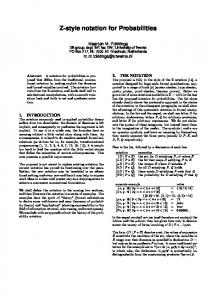
Kooi’s system describes the effects of announcements !A of propositions that are true now, as happens in straightforward conversations where we accept what the source is telling us. Thus, one updates prior probabilities with nonprobabilistic new information. But what if the source is unreliable, and hence the new information itself is probabilistic? Suppose we meet a Liar, a kid whom gives us information about A (“I stole a cookie”). If A is the case, and the Liar speaks at all, she says “A” with probability 0.3, but “¬A” with probability 0.7; if ¬A is the case (that is, if she did not steal the cookie), she has no reason to lie, and she will speak the truth. In this case, we must distinguish two sorts of probability that factor into the update: (a) prior probabilities of worlds, recording our informative experience so far, but also what may be called ‘process descriptions’ for the event being observed, which require (b) occurrence probabilities for new events in worlds. Example: Monty Hall Both kinds of probability play in the well-known paradox of the Quizmaster. Once you have chosen Door 1, the Quizmaster opens Door 2 with probability 1/2 if the car is behind Door 1, with probability 6
Nature acts 1 3
car behind 1
1 3
car behind 2
1
car behind 3
1
I choose 1 1 2
1 3
I choose 1
1 2
1 I choose 1
1
Q opens 2 Q opens 3
Q opens 3
1 Q opens 2
Figure 1: A tree for the Monty Hall Puzzle 1 if the car is behind Door 3, and with probability 0 if the car is behind Door 2. Van Benthem (2003) takes this scenario as a point of departure, depicted in the tree of possible events sequences in Figure 1. This tree is precisely the sort of semantic model that is produced by repeated dynamic-epistemic product update. Accordingly, van Benthem introduces action models of publicly observed events, standing for the ‘scenario’ driving the puzzle. These actions come with occurrence probabilities in worlds, which are encoded using ‘generalized preconditions’ Pre(a, w) which assign occurrence probabilities for events a in worlds w in arbitrary models. These may also be indexed to Pre(i, a, w), allowing for varying estimates by different agents. In any particular model M , the Pre(i, a, w) then yield local occurrence probabilities Pi,s (a) for individual events a at worlds s, according to agents i. This tree format with generalized preconditions provides more generality (and less explicit information) than may be desirable. In practice, worlddependence of events is often achieved in a more uniform manner by a linguistic ‘process description’ that can be part of the formal language. In Section 6 below, we will consider several such specializations. Van Benthem’s update rule now runs as follows. Product models M × A are defined just as for DEL in Section 3. The only new feature to be defined are the new probabilities in the product model: Pi , (s, a)((t, b)) for ‘accessible’ worlds (t, b) in M × A, where we have that t ∼i s in M and b ∼i a in A, while M, t |= Preb : Definition 1 (Probability Product Update Rule) Pi,s (t) × Pi,t (b) (u,c)∈Di,(s,a) Pi,s (u) × Pi,u (c)
Pi,(s,a) ((t, b)) = P
7
(3)
This rule looks forbidding, but the idea is very simple, and it comes out clearly for one agent with uniform probabilities. In that case, subscripts of P operators for agent and state are superfluous, and the update rule becomes: P (t) × Pt (b) (u,c)∈D P (u) × Pu (c)
P ((t, b)) = P
(3)
The new probabilities are computed in the numerator, taking a product of the prior probability for the initial world s and the occurrence probability for the event a. This is indeed how standard textbooks compute probabilities of event sequences in our Quizmaster tree. The denominator just normalizes the probabilities assigned by taking the sum of all numerator values in all relevant cases. As for probabilistic reasoning in this setting, e.g., that involved in solving Monty Hall-style puzzles, van Benthem does not provide a complete logic. But he points out that the crucial reduction axiom can be designed by redescribing the Probability Product Update Rule in terms of the model M before the update. The index in the numerator ranges over all tuples (u, c) in Di,(s,a) . This looks at all u in Di,s satisfying the precondition Prec . Thus, the above quotient is equivalent to P {Pi,s (u) × Pi,u (c) | u ∈ Di,s &u |= Prec &u |= [A, c]ϕ} P (3′ ) {Pi,s (u) × Pi,u (c) | u ∈ Di,s &u |= Prec } This is a sort of generalized conditional probability for effects of actions. Kooi’s system for public announcement is a special case of this mechanism, and his reduction axioms drop out of (3) and (3′ ) under suitable simplifications. But also, the above Quizmaster protocol for opening doors comes out with the right intuitive outcomes – and so do effects of Liars with known reliabilities. Thus, the system agrees with standard probability theory in its valid principles. But a novel and potentially useful feature is the systematic construction of successive probability spaces. The standard picture in Bayesian conditioning is that of a current space which gets smaller and smaller as new information comes in. Product update, however, can modify the current model in more complex ways, ‘branching’ currently single worlds into different continuations. This seems helpful in practice, as the main difficulty which people have with probabilistic reasoning does not seem to be the mathematical calculus per se, but the selection of the right probability model to put this calculus to work.
5
Modelling probabilistic information change
The main point of this paper is that the preceding systems still leave out further essential aspects of probability update and its logic. In this section, we first identify a third crucial probabilistic aspect, and then go on to provide a generalized update rule. We will do this with various versions of the action model scenario, allowing more focus on the processes being modeled. At the 8
end, we also show to which extent the three different sources of probability can mimic each other.
5.1
Three sources of probability
The model of Section 4.2 performs only a partial ‘probabilization’ of DEL-style product update. But there is also a third type of uncertainty that we have not modeled yet: concerning the event that is being observed. I see you read the letter from the Agency, and I know it is either a rejection of your grant proposal or an acceptance. You know which event (“reading YES”, “reading NO”) is taking place, while I do not. Epistemic product update in its nonprobabilistic version computes the resulting differential uncertainties for you and me, which may be quite intricate. But the latter, too, can be analyzed in a more fine-grained quantitative manner in the present setting. To do that, we must distinguish, not two, but three sorts of probability: (a) prior probabilities of worlds, (b) occurrence probabilities for new events in worlds. as well as (c) observation probabilities for the current event. Perhaps I saw a glimpse of your letter, or you looked smug: and thus, I might assign probability 0.7 to your reading an acceptance rather than an rejection. A simple scenario where all three kinds of probability come together is this: Example: The Mumbling Liar You do not know whether p – Mary, your three year old daughter, took a cookie – is true or not. You assign probability 0.5 to either case. You ask Mary whether she took the cookie: you know that if she did, she will speak the truth with probability .3 (if she did not, she will, of course, not lie about that). Mary mumbles something – you did not quite get whether her answer was ‘yes’ or ‘no.’ You think that you observed a “Say-yes”-event with probability 0.8, but there is a 0.2 chance that it was “Say-no”. What should be the new probability when all this is taken into account? There are four possible worlds in the product update model: ((¬)p, “Say (¬)p”), and it seems reasonable to compute their probabilities by multiplying all three relevant probabilities: (a) the prior for the world with p or ¬p, (b) the occurrence probability for Mary’s assertion, and (c) the observation probability that the event in the pair is in fact what we observed. An interesting further feature of this three-source analysis is that the probabilities may be very different in kind. The prior may be subjective, the occurrence probability might be an objective frequency, whereas the observation probability might be subjective again. 9
This setting invites a richer style of epistemic-probabilistic update. The intended role of our three probabilities may be summarized in the following simplified notations for probabilities P (t, b) of new worlds (t, b) produced by some informational event b in a current world t. For perspicuity, we suppress denominators normalizing probability values. Kooi’s update rule basically kept the prior world probabilities in the initial model: P (t, b) = P (t) and then normalized them within the smaller set of worlds satisfying the announced formula. Van Benthem’s update rule then multiplied this also with the occurrence probability of the event at the world: P (t, b) = P (t) × Pt (b) But now, we need a format with three factors, multiplying also with an observation probability for the event that does not depend on the world: P (t, b) = P (t) × Pt (b) × P (b) We are now in a position to define this update rule explicitly over our general models so far. But this format with arbitrary probabilities Pt (b) for events b depending on worlds t in any current model M seems too general in practice. Instead, we will first define more wieldy probabilistic event models where occurrence probabilities arise in a more uniform manner.
5.2
Event models and general product update
For a start, our static epistemic-probabilistic models M are still the same as before, and so is our epistemic-probabilistic language. Indeed, we can also use the earlier DEL notation [A, e]ϕ for the effects of executing an epistemic event (A, e). But we will now redefine what we mean by such models, representing uniformly defined epistemic-probabilistic ‘events’: Definition 2 (Probabilistic event models) Probabilistic event models are structures A = (E, Φ, Pre, P ) where Φ is a set of mutually inconsistent and jointly exhaustive sentences called preconditions, Pre assigns to each ϕ ∈ Φ a probability distribution over E (we write Pre(ϕ, a) for the probability that a occurs given that ϕ is true). Finally, P is a probability function over E. This should be understood as follows. Part of the models consists in the specification of an observed process which makes events occur with certain probabilities, depending on a set of conditions Φ which cover all eventualities in a unique manner. Liars or Quizmasters are such processes, with instructions of the form ”if P holds, then do a with probability q”. But one can also think of Markov Processes or other standard probabilistic devices. The language for these conditions Φ is left open here, but in an eventual clean set-up, it would be the formal language of our dynamic-epistemic-probabilistic 10
system, used with the right set of simultaneous recursions. One can think of these processes as observer-independent, though the more ‘lush’ notational version of our approach would allow for agent-dependent occurrence probabilities, encoding their perhaps mutually distinct estimates of the occurrence probabilities. (E.g., parents’ probabilities for the veracity of their children tend to differ from those of everyone else.) The second component of the models is the probability function P , which stands for probabilities assigned by the observer as to which event actually took place. The latter feature encodes a property of the observation process. Remark: Subsuming Standard Event Models Non-probabilistic event models can be viewed as a special case of probabilistic event models, and that even in at least two ways. We could think of them as having probability measures into the two-element space 0, 1, being just the characteristic functions for the usual preconditions. If we want a partition here, we can do this for the maximally consistent sets of the relevant preconditions and their negations. The other option would be to assume an equiprobability measure for occurrence of all events whose standard epistemic preconditions are satisfied. Remark: Occurrence Probabilities We have chosen here to let the function Pre assign a probability distribution over the whole event set E. The intuition is that one and only one event will occur, as happens in epistemic product update with pairs (s, e): no ‘concurrent events’ are allowed. This means that each possible event gets a probability (if only value 0), and these probabilities must sum to 1. This stipulation does not quite fit standard product update. The latter allows for ‘dead-end worlds’ where no event can take place, as in the case of public announcement eliminating current worlds. But we can always redescribe the latter scenario by means of discarded worlds supporting some new ‘blocking action’. Alternatively, we could let the issue open how occurrence probabilities behave. In this paper, we will leave such design details open. Another related detail is that we have not put explicit old-style preconditions for events, since these can be subsumed under the occurrence probabilities. With these models, computing an update involving all three sources of probability is a straightforward generalization of earlier rules. We give a version in simplified notation, with a hint of a lush agent-indexed version: Definition 3 (Full Product Update Rule) For any static epistemic-probabilistic model M and probabilistic event model A, the product update model M × A is defined exactly as for DEL on the epistemic part, but now with a probability measure P over the set S × A of pairs of states from M and events from A. Let Φ(t) be the unique element of Φ that is true in t. We set: P ((t, b)) = P
P (s) × Pre(Φ(t), b) × P (b) u∈S,c∈E P (u) × Pre(Φ(u), c) × P (c)
(4)
Agent-indexed versions of this, indicating also the relevant models where probabilities are taken, have a numerator in the following format: 11
M ×A M Pi,(s,a) ((t, b)) = Pi,s (t) × PreA (Φ(t), b) × Pi,a (A, b),
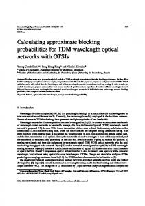
while the denominator would only sum over pairs (world, event) that are epistemically accessible in M × A from the vantage point (s, a). Here is how this update mechanism works out in practice. Example: The Mumbling Liar Again In our example of Mary taking a cookie, our initial hypothesis about the proposition p of taking the cookie is captured by a prior probability distribution 1 2
1 2
A
¬A
We then observe Mary mumbling her answer, assigning our probabilities regarding her character (if she has a reason, she lies with probability .7) and our powers of observation (we think she said p with probability .8) as above, resulting in the following probabilistic event model: A
Say A(.8)
0.3 0.7
¬A
Say ¬A(.2)
1.0
The product of our initial state with this model is as follows: 12 29
7 29
10 29
p, Say-p
p, Say ¬p
¬p, Say ¬p
This diagram is our new probabilistic information state after the whole episode. Note how it also illustrates another typical feature of product update. We do not just eliminate existing worlds or change prior probabilities, but may also construct new types of possibility. Initially, we only considered options for one single aspect of reality (Mary took the cookie, or not), after the update, we consider more complex epistemic possibilities, including information about whether she lied about it or not. In this way, the number of options may increase (from 2 to 3 in our case), even though we have in fact obtained information. The new possibilities may be viewed as possible runs of the total process represented by our probabilistic event model. Also worth high-lighting is the following feature of our update rule. Essentially, it only changes probabilities of members of the partition Φ in a probabilistic event model A. For, any given partition member ϕ of Φ defines a set 12
of worlds in the given model M where all events f have the same occurrence probabilities. Moreover, A assigns uniform observation probabilities to events f . It follows that the ratio between the new product probabilities P (s, e) and P (t, f ) in M × A for worlds s, t in the same partition cell is the same as the ratio between the old probabilities P (s) and P (t) in M . This point will return later, in our discussion of ‘weighted’ update rules. Finally, we observe that our construction can be iterated. Processes of successive observation will just compose into sequences of static epistemicprobabilistic models M , M × A, (M × A) × B, and so on. Alternatively, one can achieve the same effect as one product M × (A ◦ B), where A ◦ B is the obvious notion of composition for probabilistic event models.
5.3
Specialized protocol models and observation models
We now have a most general update format based on three kinds of probability, together with policies expressed in weights. There is an obvious further issue here. We can either phrase it philosophically, or mathematically. The question is whether these three kinds of probability are really so different as we have made them, or whether the distinctions are somewhat blurred. More technically, can one kind of probability can do the job of the other? This subsection is a digression which can be skipped without loss of continuity. It will be expanded in the complete version of this paper. 5.3.1
Protocol models
We first look at a natural specialization of probabilistic event models. The following notion describes pure probabilistic processes, such as Markov chains or agents following some fixed protocol, without encoding any information about observation probabilities of the events that form their manifestations: Definition 4 (Protocol Models) A protocol model is a probabilistic device (E, Φ, Pre), with E a set of events, Φ a finite set of disjoint propositions, and Pre a map assigning conditional probabilities Pre(ϕ, a) to events a, given any proposition ϕ from Φ. Note that we do not require the event probabilities to sum to 1 here. From a formal point of view, the effect of any probabilistic event model can be simulated by a protocol model. The following reduction ‘absorbs’ observation probabilities into modified occurrence probabilities: Theorem 2 For any probabilistic event model A = (E, Φ, Pre, P ), there is a protocol model P rot(A) = (E, Φ, Pre′ ) with the same update effect, i.e. for the following identity holds for all models M : M × A = M × P rot(A)
13
The model P rot(A) redefines its occurrence probabilities as follows: Pre′ (ϕ, a) = Pre(ϕ, a) × P (a). Clearly, the two models assign the same probabilities to worlds in the same product model. Is this just a trick, or a natural ‘remodeling’ of the initial scenario? Suppose that we have one unambiguous signal possible in each world, but observation probabilities differ. The new events have become publicly observable, but with changed occurrence probabilities – and hence they must be interpreted differently. Say the event ‘signal a occurs’ now comes to mean ‘the a-world yields an identifiable signal for me’. Whether this is intuitively attractive must be left to the modeler. Also, the new occurrence values need not yield a probability distribution over events at the worlds in the initial model M . Indeed, one can show that this is inevitable. 5.3.2
Observation models
Moving in another direction, we can also drop the occurrence probabilities from probabilistic event models, and just record observation probabilities. The result is the following notion, where we drop the ‘partition’ requirement for preconditions, as this no longer seems imperative. We do retain the old non-probabilistic preconditions of ‘classical’ action models. This represents a scenario where an agent knows that events occur or not, in a non-probabilistic manner. But she is uncertain as to which event she is actually observing. Definition 5 (Observation Model) An observation model P is a tuple (E, Pre, P ) in which Pre is a precondition map that assigns a sentence to each event in E, and P is a probability distribution over E. The relevant notion of product update is again the obvious specialization of our earlier general product rule: P (s) × P (a) P ((s, a)) = P {P (t) × P (b) | t ∈ S and u |= Pre(b)}
(5)
The function P is again a probability distribution. Again we can ask whether this, apparently much more drastic, specialization of probabilistic event models restricts expressive power. This time, the answer is not in terms of identity, but of bisimulation: Theorem 3 For any probabilistic event model A there is an observation model Obs(A) such that for any M : M × A is bisimilar to M × Obs(A).
14
A complete proof may be found in the extended version of this paper. The main idea is to create new events for Obs(A) as pairs (ϕ, e) with ϕ in Φ, and define new probabilities according to the rule P (ϕ, e) = Pre(ϕ, e) × P (e) suitably normalized by a nominator summing all relevant products of this kind. Again, to make sense of this as a re-modeling tactic, we need to interpret the new events in some plausible manner. E.g., in the Quizmaster Puzzle, this would amount to splitting the old event of ‘opening door 2’ into two different ones: opening door 2 when the car is behind door 1, and opening door 2 when the car is behind door 3. We do not commit to the advisability of this in practice. Thus, distinctions between our three kind of probabilities can be blurred. Whether these reductions have intuitive uses, however, remains to be seen. Finally, one might think that a given probabilistic event model A should be retrievable as some sort of operation on its two ‘projections’ P rot(A) and Obs(A). But this would count some probabilities twice, as we have shifted all the information form A into both projections. Nevertheless, it is easy to see that A will indeed have the same effect as the event model composition of its pure protocol part with the original occurrence probabilities and its observation part with the original observation probabilities. The fit between the two occurrences of events e in the two models is ensured by a precondition that ‘observation e’ can only happen when ‘occurrence e’ takes place. These different ways of setting up the relevant event models are also different ways of modeling our guiding scenarios, such as the Mumbling Liar. In particular, separating ‘protocol’ and ‘observation’ parts may have its uses in terms of modularity. We want to be able to identify the same process when encountered under different observational circumstances.
6
Dynamic logics of probabilistic update
In order to reason about probabilistic information change in a dynamic-epistemic format, we must extend existing axiom systems like Kooi’s with appropriate reduction axioms. In this section, we show how this can be done for our general mechanism of update with all three probability factors. Consider the probabilistic event models of Section-5, which had a partition Φ of worlds into zones with occurrence probabilities for events, and which also had observation probabilities over all events. The crucial information about our Product Update Rule will be reflected in our reduction axioms, which state when propositions get certain probabilities after an epistemic event took place. Moreover, we know already that reduction axioms express a certain harmony between the dynamic and static parts of an epistemic language. E.g., absolute probabilities after public announcement called for a language with conditional probabilities. Some experimentation with putative axioms after products with 15
event models will reveal the need for something even stronger, viz. additive probability statements of the form α1 × P (ϕ1 ) + · · · + αk × P (ϕk ) = x or even the earlier-mentioned linear inequalities of probability statements, replacing the equality by a ‘less than’ sign. More precisely, our dynamic-epistemic-probabilistic language can be defined in the following inductive format: p | ¬ϕ | ϕ ∧ ψ | ϕ ∨ ψ | Ki ϕ | [(A, e)]ϕ | α1 × P (ϕ1 ) + · · · + αk × P (ϕk ) ≤ β × P (ψ) where (A, e) is a probabilistic event model, and αi , β are rational numbers. There is a joint recursion hidden in this set-up, somewhat like that for purely epistemic product update with event models. The formulas that define the partition in our probabilistic event models come from the same language that we are defining here, but through the clause for the dynamic modalities, such models themselves enter the language again. The key reduction axiom for reasoning about product update must relate formulas of the form [(A, e)]ψ with ψ involving probabilities to assertions in terms of probabilities in the original model (M, s). For a start, we analyze the probability value P (ψ) of a formula ψ in a product model (M, s) × (A, e). The worlds in the product model where ψ holds can be divided into a finite partition consisting of sets of worlds t such that (t, f ) |= ψ in the product model, where f runs over all events in A. Fix such an event f . We must have (t, f ) epistemically indistinguishable from (s, e). Moreover, in such a pair, we clearly have that [A, f ]ψ holds in M at t. Finally, the given partition Φ in A assigns a unique proposition ϕ(t) to the world t for which A provides an occurrence probability of f in t. By our Product Update Rule, the probability of (t, f ) is then the product of three probability terms: prior-prob(t) × occurrence-prob(ϕ(t), f ) × observation-prob(f ) or, more precisely: P(M,s)×(A,e) (t, f ) := PM (t) × PreA (ϕ(t), f ) × PA (f ) Summing all this in an obvious way, we have that: P(M,s)×(A,e) (ψ) = Σf ∈A,ϕ∈Φ (PM (ϕ ∧ [A, f ]ψ) × PreA (ϕ, f ) × P (f )) Using this observation, we automatically get a reduction axiom in standard DEL style for dynamic-probabilistic assertions of the form: [A, e](P (ψ) = k)
16
in which ‘P ’ refers to the probabilities after the update, as a sum of terms referring to probabilities in the initial model M of the form: α0 × P (ϕ0 ∧ [(A, f0 )]ψ) + . . . + αn × P (ϕn ∧ [(A, fn )]ψ) = k Now the language is not yet in expressive harmony here, since we need sum terms in the static language to deal with single probability assignments after the update. However, it is easy to see that this can be solved once we provide the static language with either linear equalities or linear inequalities of probability statements. Theorem 4 The dynamic epistemic probabilistic logic of update by probabilistic event models is completely axiomatizable, modulo some given axiomatization of the logic of the chosen class of static models. The proof of this result is easy. When analyzing a statement [(A, e)](α1 × P (ϕ1 ) + · · · + αk × P (ϕk ) ≤ β × P (ψ)) we can replace the separate terms P (ϕi ), P (ψ) after the modal update operator by their equivalents as computed just before. The result is a linear inequality where the terms of the main sum may themselves contain sums. Rearranging terms, this can be brought into the form of one big sum with probabilities for formulas in M with suitable coefficients. In particular, no essential multiplication is introduced for the probability terms. Our methodology via reduction axioms yields a relative, rather than an absolute axiomatization of the full dynamic language. In particular, we cannot say without further information whether the total system will be decidable. One can take any base system of reasoning about probabilities for the chosen static models, and the reduction axioms will then also allow for reasoning about effects of dynamic actions on top of that. Here, the complexity increase is small: a straightforward reduction procedure removing dynamical modalities [!A] takes exponential time in the length of the input formula, while even a polynomial SAT -reduction is known for the dynamic logic of public announcements to basic epistemic logic. Thus, if one starts with a base calculus of low complexity, such as linear equations between terms with rational coefficients, complexity of the full dynamic logic stays low. The same would be true for the arithmetic of the real numbers with addition and multiplication, which is decidable by Tarski’s Theorem. Of course, if one starts from an undecidable base calculus, say, the arithmetic of addition and multiplication on natural numbers, the dynamic logic will be undecidable, too – but at least, it will be no worse. This concludes our discussion of logics for probability update. Evidently, there is more to be said, especially when we look at the topic of the next Section: agent-dependent ‘weighted versions’ of product update. But for now, we have at least shown that the general logic design of DEL also seems to work in a broader probabilistic setting. 17
7 7.1
Parameterizing the Update Rule Policies and weights
Our analysis so far identified three component probabilities that drive information update. But this still leaves out one more major issue. In the earliest publications on Inductive Logic in the 1950s, Carnap pointed out that update requires another component, viz. a policy on the part of agents. We have a current probability distribution, encoded in the model M . We observe a new event, encoded in an event model A. The resulting model will now depend on how much weight agents assign to the two factors: ‘past experience’ versus ‘the latest news’. The result was Carnap’s famous ‘continuum of inductive methods’. Diversity of update policies is also a key feature in modern Learning Theory (Kelly 1996), and belief revision theory (G¨ardenfors and Rott 1995). See also (Liu 2004) on diversity of update policies for different agents even inside dynamic-epistemic logic. By contrast, our updates in Section 5 essentially assigned equal weight to all factors. For instance, if one thought that ¬p was true with probability 0.9, and now observes an event a which says with probability 0.9 that p occurred, then the product rule will give both options (p, a) and (¬p, a) equal weights 0.81 in the product model M × A. But surely, other policies are possible. A conservative person will give much greater weight to the prior probabilities, a post-modern updater sheds the past whenever something new occurs, and follow the observation probabilities in the event model. Carnap modeled compromises between such extremes by assigning weights to the probabilities that go into the Update Rule. These weights seem an independent dimension of updating agents, viz. how they use given probabilistic event models. Of course, one can always absorb weights into probabilities, adjusting the given probabilities in the current models M , A to achieve the same effect with ‘equal weight’ to all three – but explicit representation of agents’ policies seems more natural.
7.2
General weighing: the ABC formula
Suppose that we want to allow agents to give different weights to the three probability factors in our update scenario. This can be done in various mathematical ways, but one convenient one would work with three numbers α, β, γ from the interval [0, 1]. These numbers represent the respective strength of the three kinds of probabilities in the light of new evidence, with 0 meaning “does not count at all” and 1 representing the judgment that this evidence is at least as good as any other. The resulting formula for the new probability values will have the following numerator: P (s, e) = P (s)α × ϕ(s)(e)β × P (e)γ and it is easy to normalize this into an over-all probability distribution again by summing over all cases in the denominator. This is our First Weighted Product Rule. 18
It is instructive to look at some special cases. Choices (1, 1, 1) for the three exponent values is just what our product update rule did. A choice (1, 1, 0) means that we ignore the observation probabilities, and so on. Thus, we can model extremely ‘conservative’ or extremely ‘progressive’ behavior, as described above. Note in particular, that a value 0 for the factor α gives each world in M equal weight, and the effect of this under our normalization procedure is the same as assuming an equiprobability distribution instead of the original prior. Still, this way of weighing raises some questions. First, it is not clear whether our particular formula is the best. We have chosen to weigh factors in product update, and then normalize everything at the end to one probability distribution. This mixes the influence of the factors α, β, γ in the denominator. An alternative would have been to consider the three separate factors as changed probability distributions by themselves. In that case, it is not the Product Update Rule itself which changes, but only its input. More precisely, define a new probability distribution P γ (e) =
(P (e))γ Σe∈E (P (e))γ
and likewise, a weighed Preβ as Preβ (ϕ, e) =
Pre(ϕ, e)β Σϕ∈Φ,e∈E (Pre(ϕ, e)β
A weighted P α (s) can be defined in the same style, as: P α (s) =
(P (s))α Σs∈s (P (s))α
Now, we can define a Second Weighted Product Rule as follows: P (s, e) = P α (s) × Preγ (Φ(s), e) × P γ (e) We will not compare the First and Second Rules in any detail here. Note that, like the former, the latter weighs all prior probabilities. In particular, this means that if α is very small, i.e. if the prior information is considered to be of little or no weight with respect to the new information, we suppress all prior information we have about relative probabilities. In the limit, with α = 0, P assigns equal probabilities to all elements of S. Next, even though it makes sense to weigh prior probabilities P (t) and also observation probabilities P (e), this seems less clear with occurrence probabilities, which seem really hard knowledge about the sort of process we are encountering? A deeper issue here is one of learning. Should not observations that we make lead to revision of hypotheses about the process? This issue arises for instance in discussion of ‘reliability’ of agents on the basis of the truth value of their assertions. These issues are discussed briefly in Section 8. Finally, it should be noted that in any single application of Product Update, weighing can always be replaced by manipulating the plain occurrence 19
and observation probabilities. But having it as a separate phenomenon allows us greater flexibility and expressiveness in describing types of agent.
7.3
Jeffrey update
Our system can deal with quite probabilistic updates on the basis of quite complex incoming information. But it meets with a challenge, so-called Jeffrey Update. Consider the following example, adapted from (Halpern 2003): Example 1 (The Dark Room) An object in a room has one of 5 possible colors, 3 of them light (red, yellow, green), 2 dark (brown, black). We have an initial probability distribution over these five cases, say, the equiprobability measure. Now we make an observation of the object, and we see that, with probability 3/4, the object must be dark. What are the new probabilities? Jeffrey Update takes this scenario as an instruction of the following form. The new probability of the object being dark must become 3/4, and that of its being light 1/4. But within those zones, the relative probabilities of the five initial cases should remain the same. Thus, Jeffrey tells us to do two things: • Change the probability values of propositions in some partition according to some stipulated values, • Stick to the old probability proportions for worlds that live within the cells of that partition. It is interesting to compare this with our Product Update scenario so far. We take an event model with ‘signal events’ for the relevant propositions (only one such event can happen in each world), and then assign them observation probabilities equal to the desired Jeffrey values. For instance, in the case of the object in the Dark Room, we could have two signals ‘Light’, ‘Dark’, with obvious occurrence probabilities 1 and 0 only, and observation probabilities 1/4, 3/4. Now, first, straight Product Update will not get the same effect here, and it is easy to see why. Its value for the probability that the object is dark will weigh two factors: the prior probability that the object was dark, and the observation probability. This will interpolate somewhere between 2/5 and 3/4. And indeed, there may be something to this. The way the Dark Room is described in (Halpern 2003), it is not so clear intuitively that one would really want to discard the prior here, in Jeffrey’s manner. Even so, Jeffrey Update is a widely accepted, and interesting rule. It also has natural counterparts in belief revision, where ‘lexicographic reordering’ of worlds according to plausibility on the basis of a new fact P makes all P -worlds better than all ¬P -worlds, but inside these two zones, the old comparison order is retained. So, our failure in subsuming such a natural scenario seems a problem. And it persists, even with our weighing method so far. Suppose that we set α to zero, and γ to 1, we get the right probabilities for the propositions ‘Light’, ‘Dark’ after the update, but the wrong probabilities for the individual worlds inside the 20
partition induced by them. The reason is that we need the old probabilities after all to compute the relative probabilities s for these worlds. More technically, the denominator for normalizing the product values in the numerator is uniform over all cases, whereas it needs to have different cases for P , ¬P in the Jeffrey Rule. We will take this observation as our cue for another style of weighing, to be discussed below. For the moment, we conclude with a few further observations. Remark 1 (One More Reduction) Another option for bringing Jeffrey Update into our fold replaces one Jeffrey step by two steps in our format. First, update with the event model corresponding to the above signals and their given observation probabilities, using weight 0 for the prior on M (i.e, one temporarily assumes an equiprobability distribution on the old worlds). Then update once more with new signal events for individual worlds whose observation probabilities are the old proportional probabilities. The best that can probably be said for this approach is that it is a trick. Remark 2 (Looking Backward versus Forward) Another major difference between our DEL style update and Jeffrey Update seems a matter of ‘temporal’ perspective. DEL describes update by preconditions for events that happen. In other words, what we learn from observing an event is what was true in order for it to happen. The reduction axioms express this backward-looking feature, analyzing preconditions for assertions. Thus, in general, we have no control over what we learn from a given event. Even a true public assertion that A is the case may by its very announcement invalidate A – though it is true that the fact that A was true at the previous stage does become common knowledge. By contrast, Jeffrey Update is more like belief revision, where a forward-looking instruction is given, in the style of ‘See to it that A’, ‘Come to believe that A’, ‘Make A have probability k’. The latter type of assertion runs into grave intuitive difficulties when A is a complex assertion containing epistemic and probabilistic operators, since it may not make sense for complex facts. But for simple factual assertions A, the ones considered in belief revision or Jeffrey Update, whose truth value does not change by an epistemic action like announcing or observing, the difference between backward-looking and forward-looking approaches seems slight.
7.4
Final weighed update rule
Our discussion of Jeffrey Update suggests another look at our earlier Weighted Product Rules. First, recall that our unweighed product update rule essentially only modifies the probabilities of the propositions from the partition Φ of the relevant probabilistic event model A. For pairs (s, t), (t, e) within one partition cell in M , it retained the prior probability ratio between s and t in the original model. Thinking along the same lines, we now modify our weighted product update rule by separating two factors in the world probabilities: (a) the probability of
21
the partition cell they are in, and (b) their own conditional probability given that cell. Weighing may be said to apply only to the first aspect here, as it concerns the main point of our update. The resulting Third Weighted Rule of Product Update reads as follows: P ((s, e)) = P (s | ϕ) × (P (ϕ))α × (Pre(ϕ, e))β × (P (e))γ We conclude by pointing out a number of special cases of interest here. • Setting all three weighing factors to 1 gives our original product update. • Setting α, β, γ = (1, 0, 0) ignores all new evidence, and produces an epistemic product model M × A where summed probability of worlds (s, e) in the product model is the same as the probability of s in M . This conservatively copies the prior onto the new model. • Likewise, setting α, β, γ = (0, 0, 1) is the opposite, extremely radical, policy where observation probabilities for e determine the probabilities for worlds (s, e). • Also of interest is α, β, γ = (0, 0, 0). Here we ignore all evidence pertaining to Φ – not just the new evidence, but also the prior evidence pertain to the elements of Φ (“Now that I have heard this, I don’t know what to think anymore”). In the resulting product model, all propositions in Φ have become equally probable. As to general features, the new weighted product rule still has the earlier feature that conditional probabilities for worlds inside partition cells do not change. If α = 1, the prior conditional probabilities of worlds with respect to elements of Φ remain unchanged. Here is a quick check. Define the probability that s was the actual state to be simply the sum of the probabilities of (s, e) in the new state: P new (s) = Σe∈E (P new ((s, e))). It now holds for any (1, β, γ) update that P new (s | ϕ) = P old (s | ϕ). But perhaps the most interesting option is this: α, β, γ = (0, 1, 1) This mimics Jeffrey update for preconditions that do not contain probability statements or epistemic operators. First we sharpen up the relevant definition. Given a pair (Φ, P ) of a set of sentences partitioning the logical space and a probability distribution P over Φ, the Jeffrey update of a probability measure P old with this new information is defined as: P new (s) = P old (s | ϕ) × P (ϕ) Now, the kind of information represented by (Φ, P ) is easily captured in an event model A = (Φ, !Φ, Pre, P ) as before with ‘signal events’ for partition members. Here we set Pre(ϕ, !ψ) = 1 iff ϕ = ψ. In Jeffrey update, the observation of 22
the new signal completely overrules any prior information about the sentences in Φ. This clearly corresponds to a weighted product update in our third version, with α, β, γ = (0, 1, 1). Thus, we have shown how our third and final weighted probabilistic update rule can describe both DEL style updates and further styles of update from the probabilistic literature. As for the update logic of our various weighted update rules, we think it can be axiomatized along the lines of Section-7 for the pure case. But perhaps the more interesting logical issue would be to have a language which can define various types of updating agent explicitly, and then state and prove features of their interaction, such as learning about other agents’ types, and choosing optimal strategies for dealing with them.
8
Some further issues: model construction, time, and reasoning
We have proposed a formal system here for update and reasoning. But its fit with reality depends crucially on how one represents given phenomena in it. The ‘art of modeling’ is not formalizable, and requires good taste as well as logic – but we will make some observations about the range of our framework.
8.1
Knowing Protocols
The modeling power of our system resides mainly in the probabilistic event models, and hence their structure deserves further attention. As we have seen before, these models really combine two different ideas: (a) an observed process, and (b) the process of observation. In Section-5, we pulled these two roles apart into ‘protocol models’ and ‘observation models’. Here, the protocol model determines what external processes can be represented: events in nature, meetings with some other epistemic agent, and so on. These agents can be quite diverse. The Quizmaster had a rule where she opens a door at random when she has a choice, but she might also have other preferences, leading to other occurrence probabilities. A Liar may lie with the same frequency all the time, or with varying frequencies about different propositions – and so on. Thus, agents can follow quite complex dynamic-epistemic-probabilistic ‘programs’, which can be represented in our protocols. The flexibility of this model also shows in the following scenario, which prima facie seems beyond it. Protocols themselves can be objects of uncertainty. An observer need not know which protocol is being run when communication takes place with another agent. Someone tells me something. Am I meeting with Liar or a Truth Teller; or, even when the truth is being told: with a cooperative Gricean, or a ‘literal’ speaker? I read of the value of some detecting device. Am
23
I dealing with a really reliable or an unreliable device?) We show how to deal with this in the non-probabilistic case: adding further probabilities is easy. Example 2 (Liar, or Truth-Teller?) Consider an encounter with an unknown agent of which we know she is either a Truth-Teller T T , or a Liar L about proposition q when it is false. Both options could be defined as a ‘program’, if more precision is needed. Now the agent tells us that “q”. How should we represent the resulting update? Think of each protocol as an event model in some obvious way. Now define a new event model whose events are ordered pairs (protocol P , possible event e in that protocol) where the precondition for this new event is that the original precondition for e holds. Moreover, we put epistemic indistinguishability relations between pairs when we cannot distinguish either the protocols or the events. Suppose that we start from a two-world model for uncertainty about q, the resulting product update will give us a new model with three indistinguishable worlds {(T T , ”says q”), (T T , ”says ¬q”), (L, ”says q)}. What this example shows is that structured event models can deal with more complex informational settings than might appear at first sight. In particular, there is no need for some new level of ‘sets of event models’, and the like.
8.2
Useful model constructions
The preceding example high-lights the importance of algebraic constructions on event models. Some are well-known from the literature, such as sequential composition A ◦ B describing the effects of first applying one event model A, and then another B, in one fell swoop. Other operations that have been mentioned are disjoint sums, representing a choice, and Kleene iteration. In fact, our treatment of uncertainty about the protocol encountered is very much like composition, between an event model having all relevant protocols as ‘events’, and one collecting their observable events. But there is also a difference, in that, intuitively, the languages for the two components need not be the same. We do not have a good view at this stage of all natural constructions on event models; but their identification, and then also the study of their valid algebraic laws, seems a definite desideratum for dynamic-epistemic logic generally. Indeed, existing systems, do some of this job, witness the key validity defining standard composition: [AoB, (e, f )]ϕ ↔ [A, e][B, f ]ϕ We have some further material on model constructions, which we keep for an extended version of this paper.
24
8.3
Temporal perspective
Our discussion of agents and protocols has a temporal dimension which goes beyond the one-step updates described in DEL-style calculi. E.g., a Liar is really someone who will keep lying at every appropriate occasion. Stating this would require a more expressive temporal language about all possible future stages of some process over time. Likewise, the whole past can play a role. A probability is often a record of past experience, and hence, even when assigned locally in some static model M , it refers naturally to the epistemic and real past that brought us there. The broader perspective here is that of epistemictemporal logics for linear or branching time, of the sort developed by Fagin, Halpern, Moses & Vardi, Parikh & Ramanujam, and others. These extended logics can describe long-term behavior of update processes over time, while also allowing for preconditions of events that crucially involve time, such as “telling the truth only on Sunday”, or “lying more often than your neighbor”. In particular, current epistemic-temporal logics model processes through the notion of a protocol’, viewed as a restriction on the set of all possible runs of the system over time. Our DEL-style protocols were simple versions of this, where possible behavior depends only on preconditions satisfied by the current state. This is quite powerful– at least, more so than leading proponents of epistemictemporal logics tend to acknowledge. But more complex behavior, like Liars lying with varying frequencies, at different times, about different propositions, would really require a richer temporal language and its associated models of potentially infinite system evolution over time. A temporal setting also raises several issues of independence between successive events, and of learning about the total system that go beyond our current framework. We will mention a few of these in Section-10.
8.4
Practical reasoning with probability
In addition to ease of modeling, there is the issue of the fit between our logics and natural reasoning with probabilities. We have described updates on current models, and indeed, this controlled view of successive probability spaces can help keep track of the information flow in many known puzzles with probabilistic reasoning. But in addition to this, in practice, one also applies algebraic rules of inference such as Bayes’ Law to get from one probabilistic assertion to another, without reference to any specific model. Our logical languages and axioms look far removed from this, since their notation seems much more baroque. Part of this comes from keeping track of many agents, which standard probabilistic calculations ignore. Part may also just be the unfamiliarity of our propositional notations like P (ϕ) = k. One could remedy some of this by adding function symbols P (ϕ) to our language, and even more dynamically, P[A!] (ϕ) describing ϕ’s probability value after truthful public announcement of A. Dynamic-epistemic key axioms in our sense then turn into more familiar-looking algebraic principles, such as the following equation:
25
P[A!] (ϕ) = P ([A!]ϕ|A) Another aspect of the comparison between logical systems and practice is computational complexity – which was discussed briefly in Section-6. The upshot was this: one can view our DEL-style systems as an addition to, rather than an alternative for, existing mathematical tools.
9
Related work
Combinations of epistemic logics and probabilistic reasoning have been studied since the 1990s (cf. van der Hoek (1992)). Fagin and Halpern (1993) and Halpern and Tuttle (1993) were our point of departure for the static case. We have also reviewed two earlier DEL-style attempts by Kooi, and van Benthem. In addition, Halpern should be mentioned as a general study of probabilistic reasoning in an epistemic-temporal setting, and in particular, the work by Gr¨ unwald and Halpern (2003) as a study of probabilistic update, including Jeffrey update. We also mention the paper by Aucher (2005) which was developed independently. Some of his conclusions seems similar to ours, whereas other features diverge (e.g., he also treats drastic forms of belief revision) – but we must leave detailed comparisons to other times, places, and agents. Finally, we mention the tradition of foundations of Bayesian reasoning and its critics (Jeffrey, Glymour, Fitelson) whose concerns and results seem very congenial to ours. Romeijn (2005) provides a first attempt by a person from the latter tradition at a fruitful confrontation with dynamic-epistemic approaches.
10
Conclusions
We have presented an analysis of three major probabilistic aspects of observing an event in the framework of dynamic-epistemic logic. The resulting distinction of prior probabilities, occurrence probabilities, and observation probabilities seems to make general sense, and it allows for a richer modular view of probabilistic update and the concomitant construction of successive new probability spaces. The resulting update system has a model theory much like that of existing ones for purely epistemic or doxastic settings. In addition, we have shown how the approach can be parametrized for different types of agent assigning different weights to these factors, thus allowing for the sort of diversity widely encountered in studies of probabilistic agents. We have also shown how one can find complete logics with reduction axioms, provided the epistemic-probabilistic base language is made rich enough. Naturally, many further questions remain, especially in a controversial area like probability. We have seen already that our approach borders naturally on a broader epistemic-temporal-probabilistic setting. And such a perspective also raises further issues, that return to the earlier sequential composition of processes. Our treatment assumed that successive events are independent. But 26
there may be various dependencies between them, either for physical reasons, as in drawing balls without replacement, or in changing ideas about the reliability of agents. The next time we encounter the agent, we may have changed our views about her reliability on the basis of what she said last time. More generally, our approach has ignored methods for learning as studied in formal learning theories, not just about local facts and agents’ information about them, but about more general features of the total system and its evolution over time. From this perspective, our system may even have the disadvantage of being too ‘smooth’: it can accommodate virtually every sort of event by adapting probabilities, provided its occurrence does not have zero probability. In the latter case, however, we experience an epistemic ‘jolt’, of the sort that occurs in belief revision when encountering a contradiction. Connections between probabilistic update and drastic forms of belief revision are beyond the ambit of this paper.
11
Acknowledgments
This work goes back to various discussions between the authors over the past few years. In particular, we thank the audiences at the Edinburgh ESSLLI Workshop on Belief Revision (August 2005), the ILLC Probability and Update Workshop ‘Meet the Bayesians’ (September 2005), the ILLC-Stanford Update Day (September 2005), and the ILLC Graduate Update Seminar (October-November 2005) for their responses to ‘talk versions’ of this paper.
References Aucher, G. (2005). How our beliefs contribute to interpret actions. Accepted as a full paper at the 4th International Workshop of Central and Eastern Europe on Multi-Agent Systems (CEEMAS05). To appear in the Lecture Notes in Artificial Intelligence published by Springer-Verlag. Baltag, A., L. S. Moss, and S. Solecki (1998). The logic of common knowledge, public announcements, and private suspicions. In I. Gilboa (Ed.), Proceedings of the 7th conference on theoretical aspects of rationality and knowledge (TARK 98), pp. 43–56. Fagin, R. and J. Y. Halpern (1993). Reasoning about knowledge and probability. Journal of the ACM 41 (2), 340–367. G¨ ardenfors, P. and H. Rott (1995). Belief revision. In Handbook of logic in artificial intelligence and logic programming (Vol. 4): epistemic and temporal reasoning, pp. 35–132. Oxford, UK: Oxford University Press. Gerbrandy, J. D. (1998). Bisimulations on Planet Kripke. Ph. D. thesis, University of Amsterdam. ILLC Dissertation Series DS-1999-01. Gr¨ unwald, P. and J. Y. Halpern (2003). Updating probabilities. Journal of AI Research 19, 243–278. Halpern, J. Y. (2003). Reasoning about Uncertainty. The MIT Press. 27
Halpern, J. Y. and M. R. Tuttle (1993). Knowledge, probability, and adversaries. Journal of the ACM 40 (4), 917–962. Kelly, K. (1996). The Logic of Reliable Inquiry. Oxford: Oxford University Press. Kooi, B. (2003). Probabilistic dynamic epistemic logic. Journal of Logic, Language and Information 12 (4), 381–408. Liu, F. (2004). Dynamic variations: Update and revision for diverse agents. Mol Thesis, ILLC publication. Plaza, J. A. (1989). Logics of public communications. In M. L. Emrich, M. S. Pfeifer, M. Hadzikadic, and Z. W. Ras (Eds.), Proceedings of the 4th International Symposium on Methodologies for Intelligent Systems, pp. 201– 216. Romeijn, J. W. (2005). Dutch books and epistemic events. talk presented at the Interfacing Probabilistic and Epistemic Update workshop in Amsterdam. van Benthem, J. (2003). Conditional probability meets update logic. Journal of Logic, Language and Information 12 (4), 409–421. van Benthem, J., J. van Eijck, and B. P. Kooi (2005). Logics of communication and change. Submitted. van der Hoek, W. (1992). Modalities for Reasoning about Knowledge and Quantities. Ph. D. thesis, Vrije Universiteit Amsterdam.
28