Jan 13, 2015 - AbstractâBit-flipping decoding of LDPC codes is of low complexity but gives inferior performance in general. We propose new checksum ...
IEEE TRANSACTIONS ON COMMUNICATIONS
1
Dynamic Weighted Bit-Flipping Decoding Algorithms for LDPC Codes
arXiv:1501.02428v2 [cs.IT] 13 Jan 2015
Tofar C.-Y. Chang, Student Member, IEEE and Yu T. Su, Senior Member, IEEE emails: {tofar.cm96g, ytsu}@nctu.edu.tw.
Abstract—Bit-flipping decoding of LDPC codes is of low complexity but gives inferior performance in general. We propose new checksum weight generation and flipped-bit selection (FBS) rules to enhance their performance. From belief propagation’s viewpoint, the checksum and its weights determine the beliefs a check node (CN) passes to its connected variable nodes (VNs) which then update their beliefs about the associated bit decisions by computing the corresponding flipping functions (FFs). Our FF includes a weighted sum of checksums but unlike existing FFs, we adjust the weights associated with each checksum in every decoding iteration with some beliefs inhibited if necessary. Our new FBS rule takes more information into account in determining the bits to be flipped. These two modifications represent our efforts to track more closely the evolutions of both CNs and VNs’ reliabilities. To reduce the decoder complexity, we further suggest two selective weight-updating schedules. Different combinations of the new FBS rule and known or new FFs offer various degrees of performance improvements. Numerical results indicate that the decoders using the new FF and FBS rule yield performance close to that achieved by the sum-product algorithm and the reducedcomplexity selective weight-updating schedules incur only minor performance loss. Index Terms—LDPC codes, belief propagation, bit-flipping decoding, flipped bit selection.
I. I NTRODUCTION LDPC codes have been shown to asymptotically give nearcapacity performance when the sum-product algorithm (SPA) is used for decoding [1]. Gallager proposed two alternatives that use only hard-decision bits [2]. These so-called bitflipping (BF) algorithms flip one or a group of bits based on the values of the flipping functions (FFs) computed in each iteration. The FF associated with a variable node (VN) is a reliability metric of the corresponding bit decision and depends on the binary-valued checksums of the VN’s connected check nodes (CNs). Although BF algorithms are much simpler than the SPA, their performance is far from optimal. To reduce the performance gap, many variants of Gallager’s BF algorithms have been proposed. Most of them tried to improve the VN’s reliability metric (the FF) and/or the method of selecting the flipped bits, achieving different degrees of bit error rate (BER) and convergence rate performance enhancements at the cost of higher complexity. The class of weighted bit-flipping algorithms [3]–[6] assign proper weights to the binary checksums. Each weight can be regarded as a reliability metric on the corresponding checksum and is a function of the associated soft received channel values. Another approach called gradient descent bit-flipping (GDBF) algorithm was proposed recently [8]. Instead of using a weighted checksum based FF, the GDBF algorithm derives
its FF by computing the gradient of a nonlinear objective function which is equivalent to the log-likelihood function of the bit decision with checksum constraints. It was shown that the GDBF algorithm outperforms most known WBF algorithms when the VN degree is small. For the WBF algorithms, the weights are decided by the soft received channel values and remain unchanged throughout the decoding process. Since the weights reflect the decoder’s belief on the checksums which, in turn, depend on those of the associated VNs’ FF and bit decisions, the associated checksum weights should be updated accordingly. In this paper, we present dynamic weighted BF (DWBF) algorithms that assign dynamic checksum weights which are updated according to a nonlinear function of the associated VNs’ FF values. As we shall show, the nonlinear function has the effects of quarantining unreliable checksums while dynamically adjusts the more reliable checksums’ beliefs. We also suggest two selective weight-updating schedules to provide different performancecomplexity trade-offs. The single-bit BF algorithms flip only the least reliable bit thus result in slow convergence rates. For this reason, many a multiple-flipped-bit selection rule was suggested [8], [9]–[14]. By simultaneously flipping the selected bits, a BF decoder can offer rapid convergence but, sometimes, at the expense of performance loss. A bit selection rule may consist of simple threshold comparisons or include a number of steps involving different metrics. It is usually designed assuming a specific FF is used and may not be suitable when a different FF or metric is involved. As the FF value may not provide sufficient statistic for making a tentative bit decision, we propose a new flipped-bit selection (FBS) rule that takes into account both the FF value and other information from related CNs. The efficiencies of using the proposed checksum weight, FF, weight-updating schedules, and FBS rule jointly or separately with existing designs are evaluated by examining the corresponding numerical error rate and convergence behaviors. We show that our single-bit DWBF algorithm provides significant performance improvement over the existing single-bit GDBF and WBF algorithms. Our FBS rule works very well with different FFs and outperforms known FBS rules. Moreover, the selective weight-updating schedules suffer little performance degradation while offer significant complexity reduction when the CN and VN degrees are small. The rest of this paper is organized as follows. In Section II, we define the basic system parameters and give a brief overview of various BF decoders and the associated FBS rules. In Section III, we introduce our checksum weight updating
2
IEEE TRANSACTIONS ON COMMUNICATIONS
rule and the associated FF. Two weight-updating schedules, the DWBF algorithm and its performance along with some other single-bit algorithms’ are presented in Section IV. We develop a new FBS rule and analyze different decoders’ complexities in Section V. The error rate and convergence behaviors of various multi-bit BF decoders using the new FBS rule is also given in the same section. Finally, conclusion remarks are drawn in Section VI.
II. BACKGROUNDS
AND
R ELATED W ORKS
A. Notations and the Basic Algorithm We denote by (N, K)(dv , dc ) a regular binary LDPC code C with VN degree dv and check node (CN) degree dc , i.e., C is the null space of an M × N parity check matrix H = [Hmn ] which has dv 1’s in each column and dc 1’s in each row. Let u be a codeword of C and assume that the BPSK modulation is used so that a codeword u = (u0 , u1 , · · · , uN −1 ), ui ∈ {0, 1}, is mapped into a bipolar sequence x = (x0 , x1 , · · · , xN −1 ) = (1 − 2u0 , 1 − 2u1 , · · · , 1 − 2uN −1 ) for transmission. The equivalent baseband transmission channel is a binary-input Gaussian-output channel characterized by additive zero-mean white Gaussian noise with two-sided power spectral density of N0 /2 W/Hz. Let y = (y0 , y1 , · · · , yN −1 ) be the sequence of soft channel values obtained at the receiver’s coherent matched filter output. The sequence z = (z0 , z1 , · · · , zN −1 ), where zi ∈ {0, 1}, is obtained by taking hard-decision on ˆ = (ˆ each components of y. Let u u0 , u ˆ1 , · · · , uˆN −1 ) be the tentative decoded binary sequence at the end of a BF decoding iteration. We compute the syndrome (checksum) ˆ · H T (mod 2). We vector s = (s0 , s1 , · · · , sM−1 ) by s = u further denote the nth VN by vn , the set of indices of its connecting CNs by M(n), and the set of indices of the VNs checked by the mth CN cm by N (m). The indices of CNs in M(n) are determined by the nonzero elements of the nth column of H whereas those in N (m) are by the mth row of H. A generic BF decoding algorithm can be described by Algorithm 1 below which involves three important parameters, lmax , the maximum iteration number, En , the FF, and B, the index set of the flipped bits, or the flipped bit (FB) set for short. This algorithm performs two basic tasks: 1) computing En ’s (Step 2) and 2) generating the FB set B (Step 3). Most earlier works focused on improving either 1) or 2). An FF, sometimes referred to as cost function or inversion function [8], is used as a reliability metric on a VN’s tentative decision. Given the FF values and the flipped bit selection (FBS) rule, we select a set of VNs and flip the corresponding tentative decisions (bits). Choosing the most unreliable bits or the bits whose FF values exceed a threshold are the two most popular rules. For the former rule, usually only one bit is flipped if the softvalued channel information is employed in the FF, resulting in slow convergence. By contrast, the latter rule often gives faster convergence rate but possibly at the cost of performance loss. We briefly review the known FFs and FBS rules in the following paragraphs.
Algorithm 1 Bit-Flipping Decoding Algorithms ˆ = z, and compute wmn for each Initialization Set l = 0, u n ∈ N (m), m = 0, 1, . . . , M − 1. Step 1 For m = 0, 1, . . . , M − 1, compute X u ˆn Hmn (mod 2). (1) sm = n∈N (m)
ˆ; If s = 0 or l = lmax , stop decoding and output u otherwise, let l = l + 1. Step 2 For n = 0, 1, . . . , N − 1, compute the FF En . Step 3 Use the FFs obtained in Step 2 to update the flipped bit set B Step 4 Flip u ˆn for all n ∈ B and go to Step 1.
B. Flipping Functions of BF Decoding Algorithms Gallager proposed that a simple sum of binary checksums be used as the FF [2] X (1 − 2sm ). (2) En = − m∈M(n)
(2) implies that the FF value is inversely proportional to the bit decision reliability as it is an increasing function of the number of nonzero checksums (i.e., unsatisfied check nodes, UCNs). By taking into account soft-valued channel information and assigning checksum weights, later modifications of Gallager’s FF can be described by the following general formula X wmn (1 − 2sm ), (3) En = −α1 · φ(ˆ u n , yn ) − m∈M(n)
where α1 > 0, φ(ˆ un , yn ) is a reliability metric involving channel value and/or bit decision, and, to be consistent with (2), wmn ≥ 0. For the weighted BF (WBF) algorithm [3], φ(ˆ u n , yn ) = 0 and wmn is wmn =
min
n′ ∈N (m)
|yn′ |,
(4)
The modified WBF (MWBF) algorithm [4] has φ(ˆ u n , yn ) = |yn | while the improved MWBF (IMWBF) algorithm [5] uses the same φ(ˆ un , yn ) but replaces the checksum weight by wmn =
min
n′ ∈N (m)\n
|yn′ |
(5)
for the belief passed from cm to vn should exclude that originated from vn . For the reliability ratio based WBF (RRWBF) algorithm [6], φ(ˆ un , yn ) = 0 and � �−1 ′ |yn | wmn = 1/wmn = β , (6) maxn′ ∈N (m) |yn′ | where P
β
is the normalizing factor to ensure that ′ w n∈N (m) mn = 1. The GDBF algorithm of Wadayama et al. [8] applies the gradient descent method to minimize f (ˆ u) = −
N −1 X n=0
yn (1 − 2ˆ un ) −
M−1 X m=0
(1 − 2sm )
(7)
SUBMITTED PAPER
3
with respect to (1 − 2ˆ un ) and obtains the FF X (1 − 2sm ), En = −yn (1 − 2ˆ un ) −
(8)
m∈M(n)
which is equivalent to assigning α1 = 1, φ(ˆ un , yn ) = yn (1 − 2ˆ un ), and wmn = 1 in (3). C. Flipped Bit Selection Rules For the algorithms mentioned in the Section II-B, only the bit(s) related to the VN having the largest FF value En is (are) flipped in each iteration, i.e., the FB set is B = {n|n = arg max Ei }. i
(9)
As mentioned before, |B| = 1 and the corresponding convergence is often very slow if En has a soft-valued information term. Flipping several bits in each iteration simultaneously can improve the convergence speed. The simplest FBS rule for multi-bit BF decoding uses the FB set B = {n|En ≥ ∆},
(10)
where the threshold ∆ can be a constant or be adaptive. The optimal adaptive threshold was derived by Gallager [2], assuming that no cycle appears in the code graph. Since practical finite-length LDPC codes usually have cycles and the optimal thresholds can only be found through time-consuming simulations, two ad-hoc methods which automatically adjust ∆ were suggested in [11] and [14]. In the adaptive threshold BF (ATBF) algorithm [11], the initial ∆ is found by simulation and subsequent thresholds are a monotonically non-increasing function of the decoding iterations. The adaptive MWBF (AMWBF) algorithm [14] adjusts the threshold by � � wH (s) , (11) ∆ = E ∗ − |E ∗ | 1 − M where E ∗ = maxn En and wH (s) is the Hamming weight of the syndrome vector s. ˆ may reappear Sometimes, a tentative decoded vector u several times during the decoding process and form a decoding loop. This may be caused, for example, by the event that an even number of bits associated with a CN are flipped, leading to an unchanged checksum and then oscillating bit decisions. To eliminate the occurrence of loops, the AMWBF algorithm includes the loop detection scheme of [7] in its FBS rule so that if a loop is detected, the most reliable bit in B is removed. The parallel weighted BF (PWBF) algorithm [9] tries to reduce the loop occurrence probability by having every UCN (sm = 1) send a constant flip signal (FS) to its least reliable linked VN (based on the FF of the IMWBF algorithm) and flips the bits in B = {n|Fn ≥ ∆FS }, where ∆FS is a constant optimized by simulations, X qmn sm , Fn = m∈M(n)
and qmn is given by ( 1, qmn = 0,
n ∈N (m)
.
(14)
otherwise
Since the above remedy can only eliminate loops with a certain probability, the improved PWBF (IPWBF) algorithm employs the loop detection scheme of [7] and when a loop is detected, it removes the bit(s) receiving the smallest Fn from B. This algorithm also adds a bootstrapping step and a delay-handling procedure to further improve the bit selection accuracy but achieves limited improvement for the codes with high column degrees such as Euclidean geometry (EG) LDPC codes. A hybrid GDBF (HGDBF) algorithm was proposed in [8]. In this algorithm, single- and multi-bit BF decoding is performed alternatively and an escape process is used for preventing the decoding process from being trapped in local minima/loops. Two extensions of the HGDBF algorithm were considered in [12] and [13] which require less complexity at the expense of inferior performance. III. C HECKSUM B ELIEF AND DYNAMIC W EIGHTS A. BF Decoding and Checksum Weights In line with the belief propagation (BP) based SPA, En is similar to the total log-likelihood ratio (LLR) of vn and −wmn (1 − 2sm ) in (3) is analogous to the belief sent to vn by cm . Unlike SPA, however, for (4)-(6) and (8), the latter remains unchanged unless an u ˆn , n ∈ N (m) has been flipped, which leads to a sign change of the belief. The general FF format, (3), includes two major terms that represent the decoder’s belief of a bit’s tentative decision based respectively on its channel value (or the correlation of the channel value and tentative decision) and the beliefs on the related checksums. Since the channel values remain fixed, the checksum term should be given adjusted weights at least in the later iterations when the beliefs on checksums change. Although the flipping operation changes the reliability metric of u ˆn and the related checksums, all the FFs used in known BF decoders use static wmn thereby can neither reflect the dynamic of VNs’ belief propagations nor offer self-adjustment capability in accurately updating bit reliability information. We present dynamical weight generation method in this section. B. Dynamic Weights and New Flipping Function The review on BF algorithms in Section II indicates clearly that the FF value is a proper explicit or implicit reliability metric of a VN’s decision. As a checksum in turn is a function of the associated VNs’ decisions, the corresponding checksum weights should be updated according to the current FF values. A reasonable candidate checksum weight is therefore given by (l) rmn =
(12) (l)
(13)
n = arg ′ max En′
min
n′ ∈N (m)\n
(l)
−En′ ,
(15)
where En is the FF value of vn in the lth iteration. However, (15) may result in negative weights which is inconsistent with (2) and (3); both are increasing functions of the nonzero
4
IEEE TRANSACTIONS ON COMMUNICATIONS
checksum number. To have proper positive checksum weights based on En , we consider the likelihood ratio Pr(En |H0 ) Λ(En ) = , Pr(En |H1 )
(16)
H0 H1
π1 (C01 − C11 ) π0 (C10 − C00 )
(17)
n ∈N (m)\n
where Ω(x) =
�
x − η, 0,
x≥η . x η, the decoder is more likely to have made a correct bit decision u ˆn whose reliability is proportional to −En ; otherwise, the decision is probably incorrect. The foregoing discussion and the aim to have a weight updating rule reflecting a more accurate relation among bit decision, FF, and checksums, as elaborated in more details below, suggest that we modify (15) as � � (l) (l) (l) Ω(−En′ ), (18) rmn = Ω ′ min −En′ = ′ min n ∈N (m)\n
Pr( E
10th Iter.
where H0 and H1 denote the hypotheses that u ˆn = un and u ˆn 6= un , respectively. The conditional probability density function (pdf), Pr(En |Hi ), is the pdf of those En ’s associated with a correct or incorrect tentative bit decision at a given iteration. It is to be interpreted as a conditional pdf averaged over all VNs. The basic decision theory tells us that the optimal decision rule is given by Λ(En ) ≷
0.07
(19)
Fig. 1: Conditional FF distributions for the IMWBF algorithm in decoding MacKay (816,272)(4,6) LDPC code (816.44.878 [16]), SNR = 4.0 dB.
The clipping operator, Ω(x), besides ensuring only positive weights are used, can be interpreted as the decision for a CN to send no message to other linked VNs when the associated FF values fail to exceed the threshold, which bears the flavor of “stop-and-go” algorithms that pass a CN-to-VN belief only if it is deemed reliable. Note that a checksum sm is determined by dc bit decisions, and if sm = 0 and there is only one unreliable decision u ˆn (-En < η) among VNs in N (m), the checksum is likely to be valid and the decision is in fact correct. Hence cm should modify En to increase Λ(En ) (l) but not pass its beliefs −rmn′ (1 − 2sm ) to other connected ′ (reliable) VNs (n ∈ N (m) \ n). In doing so, En has a local (among N (m)) maximum FF decrease and the probability of reversing the bit decision is reduced. On the other hand, if sm = 1, u ˆn is likely to be only local incorrect decision, the above rule will result in a local maximum FF increase and thus a higher probability of being flipped. When more than one −En , n ∈ N (m) are clipped, no belief is sent from cm as the checksum itself is unreliable. The temporary suspension of some message propagation induced by Ω(x) also has the desired effect of containing the damage an incorrect belief may have done and preventing the decoder from being trapped in a local minimum. The above discourse confirms that (19) does fulfill the goal that weight updating should have FFs, checksums, and bit decisions join a cohesive effort in improving the performance of a BF decoder. The FF defined by (3) using recursive weight update rule P (18) tends to make the check belief part of the FF, − m∈M(n) wmn (1−2sm ), starts to grow exponentially after most of the correctable bits were flipped and the number of UCNs decreases to just a few. It is conceivable that these estimates should be given different weight with more remote estimates having less weights. This can be done by having the check belief multiplied by a damping factor, 0 < α2 < 1, as can be found in many recursive adaptive filters. As for the optimal clipping threshold η, we are unable to determine since the closed-form expressions for Pr(En |Hi ) are practically unobtainable for reasons mentioned before. Some simulation
SUBMITTED PAPER
5
efforts, however, indicate that η is close to 0 for several BF decoders, independent of signal-to-noise ratio and the iteration of interest. With the above ideas in mind, we consider a new FF based on (18) and (19) using η = 0: X (l−1) rmn (1 − 2sm ), (20) En(l) = −yn (1 − 2ˆ un ) − α2 m∈M(n)
where 0 < α2 < 1 is a positive damping constant to be optimized by numerical experiments. IV. N EW S INGLE -B IT BF D ECODING A LGORITHMS In this section, we introduce a class of single-bit dynamic weighted BF (S-DWBF) decoding methods based on the checksum weight (18), the FF (20), and three different weight-updating schedules. These schedules provide trade-offs between computational complexity and error-rate performance.
(a) Selective weight updating schedule A.
A. Single-DWBF Decoding and Weight-Updating Schedules Combining (18) and the new FF (20), we obtain the DWBF algorithm or, for simplicity, Algorithm 2. Algorithm 2 DWBF Decoding Algorithm (l)
ˆ = z. Initialize rmn by (5) for each Initialization Set l = 0, u (l) n ∈ N (m), m = 0, 1, . . . , M −1 and let En = −yn (1−2ˆ un ) for n = 0, 1, . . . , N − 1. Step 1 Compute sm for all m = 0, 1, . . . , M − 1. If s = 0 or ˆ ; otherwise, let l = lmax , stop decoding and output u l = l + 1. (l) Step 2 For n = 0, 1, . . . , N − 1, compute En by (20). (l) (l) Step 3 Update B and ∀n ∈ B, flip uˆn and let En ← −En . (l) Step 4 For all n ∈ N (m), m = 0, 1, . . . , M − 1, update rmn by (18) and go to Step 1. For hard-decision decoding, −yn (1 − 2ˆ un ) in (20) is re(l) placed by −(1 − 2zn )(1 − 2ˆ un ) and rmn is initialized as 1. In Step 3, we invert the sign of the flipped VNs’ FF values (l) before computing new rmn ’s. When we consider the FB set (9), Algorithm 2 flips only one bit (i.e., |B| = 1) at each iteration. Nevertheless, most FF values will change because of the recursive nature of (18) and (20). Therefore, in Step 4, we need to update the checksum beliefs for almost all CNs. This is one of the prices we have to pay when the dynamic weights instead of the conventional constant weights are assigned to the checksums. To distinguish from other updating rules to be discussed in the following paragraphs, we call this updating rule as the full weight-updating (belief-propagation) schedule (FWUS) and the resulting decoding algorithm as the S-DWBF-F algorithm for simplicity. To lessen the computing load of FWUS, we reduce the number of updated beliefs by prioritizing the CNs’ beliefs and update only those with higher priority. We first notice that, to ensure that the newest updated information be broadcasted, the weights of the flipped bit’s linked checksums should have the highest updating priority. Furthermore, for those VNs whose FF values change from
(b) Selective weight updating schedule B. Fig. 2: The TEFGs for two different selective weight-updating schedules.
one side of the clipping threshold η of (19) to the other side and undergo a reliability inversion, their related checksum weights should be renewed as well. With these considerations, the selective weight-updating schedule A (SWUS-A) updates only those checksums (CNs) whose indices lie in (l)
GA
,
{m|m ∈ M(n), n ∈ B} ∪{m|m ∈ M(n), (−En(l) − η)(−En(l−1) − η) < 0, n = 0, 1, . . . , N − 1}.
The time-expanded factor graph (TEFG) shown in Fig. 2(a) is a simple example illustrating how SWUS-A behaves, (l) assuming that the only VN which generates GA = {1, 2} is v4 . We denote this VN by ●, the CNs visited (selected) by the schedule by ■, and the VNs which receive new CN beliefs by �. When the DWBF algorithm is used along with (9) and SWUS-A, we substitute Step 4 of Algorithm 2 by (l) (l) Step 4 Update GA , and then update rmn by (18) ∀n ∈ N (m), (l) (l−1) (l) (l) m ∈ GA and let rmn = rmn ∀n ∈ N (m), m 6∈ GA . Then, Go to Step 1. The resulting decoder is called the S-DWBF-A algorithm. Since only a few VNs received updated beliefs from the selected CNs, some En ’s are likely to remain constant for many iterations (e.g., v3 ) or even during the whole decoding process. To spread the updated beliefs to more VNs, we expand (l) (l) the updated CN set to include both GA and GB , {m|m ∈
6
IEEE TRANSACTIONS ON COMMUNICATIONS
(l)
IMWBF GDBF RRWBF
0.1
S-DWBF-A S-DWBF-B S-DWBF-F 0.01
SPA
BER
1E-3
1E-4
1E-5
1E-6 2
The performance of the known single-bit BF algorithms and S-DWBF-A/B/F algorithms for MacKay (816, 272)(4, 6) rate0.333 LDPC code (816.44.878 [16]) and (1023, 781)(32, 32) rate-0.763 EG-LDPC code are plotted in Figs. 3 and 4 where we refer to these two codes as Code 1 and 2, respectively. The performance of SPA or the normalized BP (NBP) [15] is also given there for reference purpose. Fig. 3 shows the BER performance of Code 1 with lmax = 150. For the S-DWBF-A, S-DWBF-B, and S-DWBF-F decoders, the numerically-optimized α2 values are 0.66, 0.44, and 0.35 whereas for the IMWBF decoder, we found α1 = 0.2. Our extensive simulation concluded that the optimal reliability threshold η in (19) is close to 0, whence η = 0 is used for all DWBF algorithms. At BER=10−5 , we observe that the SDWBF-B and S-DWBF-F algorithms have 2.5 dB and 2.6 dB gains against the RRWBF algorithm; the simple S-DWBF-A algorithm achieves a much smaller 0.7 dB gain as it limit its weight update to a very limited range. The performance of Code 2 with lmax = 50 is shown in Fig. 4. Unlike Code 1, Code 2 has a much higherPdv , and the check belief part of the GDBF algorithm’s FF, − m∈M(n) (1−2sm), thus dominates the FF value after a few iterations and its performance is similar to that of Gallager’s BF algorithm, especially when SNR is high. To improve its performance we insert a damping
4
5 b
0
6
7
(dB)
Fig. 3: BER performance of several single-bit BF (S-BF) decoders as a function of SNR for Code 1.
IMWBF GDBF RRWBF S-DWBF-A
0.01
S-DWBF-B NBP
1E-3
1E-4
1E-5
1E-6
2.6
B. Performance of S-DWBF Decoding Algorithms
3
E /N
BER
(l)
M(n), n ∈ UA }, where UA , {n|n ∈ N (m), m ∈ (l−1) } and call this updating schedule as the selective weightGA updating schedule B (SWUS-B). For this expanded schedule, (l) the beliefs received by the VNs connected to the CNs in GA , not just the one selected for flipping, will be forwarded to their connecting CNs in the following iteration. Fig. 2(b) illustrates the expanded updating range by indicating the extra visited (l) CNs (those whose indices lie in GB ) with the symbol �. The DWBF algorithm with the SWUS-B schedule replaces the Step 4 of Algorithm 2 by (l) (l) Step 4a Update UA and GB . (l) (l) Step 4b Update GA and then update rmn by (18) ∀n ∈ N (m), (l) (l−1) (l) (l) m ∈ {GA ∪ GB } and let rmn = rmn ∀n ∈ N (m), (l) (l) m 6∈ {GA ∪ GB }. Go to Step 1. Similar to the previous case, the resulting algorithm is called the S-DWBF-B algorithm. Table I lists the average number of visited CNs (to update checksum weights) and VNs (to compute FF) per iteration per flipped bit or FF inversion for the different weight updating schedules. As expected, the SWUS-A/B need much less computational complexity and this reduction is more impressive when dc and dv are small. Note that for the expanded schedule (l) SWUS-B, the VNs in UA may be linked to a common set of (l) (l) CNs and GA ∩ GB can be nonempty if the code graph has short cycles. As a result, the practical average numbers of the visited CNs and VNs for SWUS-B is much less than those shown in Table I which assumes a cycle-free code. However, it can be shown that when the code girth is larger than 8 (10), the actual average visited CN (VN) number is equal to that of a cycle free code.
2.8
3.0
3.2
3.4
3.6
E /N b
0
3.8
4.0
4.2
4.4
(dB)
Fig. 4: BER performance of several S-BF decoder as a function of SNR for Code 2.
factor α3 so that (8) becomes En = −yn (1 − 2ˆ un ) − α3
X
(1 − 2sm ).
(21)
m∈M(n)
This modification is equivalent to multiplying the second summation of (7) by α3 and the damping factor is analogous to the Lagrange multiplier in (the checksum) constrained optimization. The optimal α3 for (21) is close to 1/17 for Code 2. Referring to (3), the IMWBF algorithm uses α1 = 1.8 and the S-DWBF-A (B) decoder uses α2 = 0.33 (0.3) in (20). Due to the high VN/CN degrees of Code 2, almost all CNs are updated by S-DWBF-B algorithm after two or three iterations, yielding performance similar to that of the SDWBF-F decoder. The same figure shows that the S-DWBF-A decoder provides about 0.25 dB performance gain with respect to the IMWBF decoder at BER = 10−5 and the S-DWBF-B algorithm offers additional 0.1 dB gain. Table II presents the average number of CNs visited (in the associated ETFGs) by different schedules, normalized by the total number of frames simulated (106 ) for Code 1
SUBMITTED PAPER
7
TABLE I: Complexity of Weight Updating Schedules Number of Visited CNs Number of Visited VNs
SWUS-A dv min [dv (dc − 1) + 1, N ]
SWUS-B min [dv (dv − 1)(dc − 1) + 2dv , M ] min{dv (dv − 1)(dc − 1)2 + 2[dv (dc − 1) + 1], N }
TABLE II: Average Number of Visited CNs in S-DWBF algorithms Code 1 (M = 544); SNR = 4 dB Iteration S-DWBF-A S-DWBF-B 10 15.7 137.2 30 10.1 88.7 50 8.3 76.4 Code 2 (M = 1023); SNR = 3.6 dB Iteration S-DWBF-A S-DWBF-B 5 68.7 1023.0 10 38.7 1023.0 20 32.3 1002.5
Pr( E
| H )
Pr( E
| H )
n
0.06
n
0
1
20th Iter.
0.05 10th Iter.
0.04 30th Iter.
0.03
FWUS M N
V. N EW F LIPPED -B IT S ELECTION M ETHOD In Section II, we mentioned that (10) is a simple set for selecting multiple flipped bits. In practice, it is necessary to add the option B = {n|n = arg maxi Ei } in case B = ∅. Such an FBS rule is labeled as the M1 FBS rule in the subsequent discussion. Recall that the PWBF algorithm uses the FF of the IMWBF algorithm as the VN reliability metric with the FB set (12) determined by the FS count Fn of (13). That is, a CN sends a flip signal to its most unreliable linked VN only and the VNs which receive sufficient number of reliability warnings (flip signals) shall be flipped. It turns out that, with this extra filtering of VN-to-CN messages (En ’s) and selective CN-to-VN flip signal passing, the PWBF algorithm is able to outperform the IMWBF decoder in both convergence rate and error rate [9]. This performance gain motivates us to ponder if a more elaborated flipping decision strategy that uses more information can bring about further performance improvement.
10th Iter.
20th Iter.
0.02 30th Iter.
0.01
0.00 -14
-12
-10
-8
-6
-4
-2
0
2
4
E n
A. Flipping Intensity P Let Un , m∈M(n) sm , µm , maxn∈N (m) Un , λm , arg maxn∈N (m) En , and M′ (n) = {m|m ∈ M(n), λm = n}. With these notations, we define the flipping intensity (FI) of (received by) vn as X θ0 sm δ(Uλm − µm ) F˜n = m∈M′ (n)
Fig. 5: Conditional FF distributions for the S-DWBF-F algorithm in decoding Code 1, SNR = 4 dB.
and Code 2 at selected iterations. Although the S-DWBF-F algorithm has the best BER performance among the singlebit algorithms, it requires higher computational complexity. By contrast, the S-DWBF-A/B algorithms provide trade-offs between complexity and performance. Furthermore, for both selective weight-updating schedules, the number of visited CNs decreases when one proceeds with more iterations as the numbers of flipped bits and reliability-inverted VNs decreases. We plot the FF value distributions for the S-DWBF-F algorithm in Fig. 5. In contrast to Fig. 1, where the separation between the two conditional pdfs exhibits little variation, our DWBF algorithm is able to pull Pr(En |H0 ) away from Pr(En |H1 ) as the decoding process evolves. Since the reliability of a decoder decisions based on En depends on the separation (distance) between the two pdfs, the improved separation is certainly welcome. As mentioned before, we use η = 0 in (19) for all S-DWBF algorithms. Although the optimal clipping threshold is unknown. Fig. 5 does convince us that 0 is a valid and convenient choice and the FF with the proposed dynamic checksum weighting does give a much better VN reliability reference.
+θ1 sm [1 − δ(Uλm − µm )],
(22)
where θ0 > θ1 ≥ 0 and δ(x) is the Kronecker delta function. The above definition implicitly implies that F˜n = 0 if M′ (n) = ∅ and only UCNs have a say in deciding FI. It also implies that a VN has a nonzero FI only if it has the largest FF value among N (m) and if it is connected to the largest number of UCNs among its peers in N (m), the associated FI should be even higher (θ0 > θ1 ). In both cases, a UCN cm will send a non-negative message to the VN with the highest FF value in the set N (m). However, if cm is a passed CN (PCN) (sm = 0) and dc is small, it often implies that the tentative decisions of its linked VNs are all correct. Hence if the flipped bits are to be selected by checking whether the associated FI is greater than a threshold, vλm should have a smaller probability of being chosen. This can be done by having the PCN send a drag message θ2 (sm − 1). But if there is doubt that cm is connected to even incorrect bit decisions, the PCN has better not sending such a message. We decide that this is likely to be the case if Uλm 6= µm for this inequality means that at least one VN in N (m) has more connected UCNs than vλm . With UCNs and PCNs contributing opposite signals, we modify (22) for all n, 0 ≤ n < N as X [θ2 (sm − 1) + θ0 sm ]δ(Uλm − µm ) F˜n = m∈M′ (n)
+θ1 sm [1 − δ(Uλm − µm )]
(23)
8
IEEE TRANSACTIONS ON COMMUNICATIONS
where θ2 ≥ 0. On the other hand, when dc is large, it is less likely that sm = 0 automatically implies correct decisions on all its linked bits and we thus stick to (22), having no PCN to contribute to FI. Although the thresholds θi ’s can be any nonnegative real numbers, to simplify implementation, we let θi ’s be nonnegative integers such that the FI is integer-valued.
AMWBF
A simple FI-based FBS rule is to flip the bits in the FB set B = {n|F˜n ≥ ∆FI }. But the optimal threshold ∆FI is not easy to determine especially for a code with low VN degree. A smaller threshold may cause incorrect flipping decisions while a large threshold tends to slow down the convergence or even cause decoding failure as no VN meets the the flipping requirement. To overcome this dilemma, we select a relative high FI threshold and use the FB set B = {n|F˜n ≥ ∆FI } if it is nonempty. Otherwise, B = {n|Un = maxi∈T Ui } where T , {n|F˜n = maxj F˜j }. We summarize below the new FBS rule as Algorithm 3 which, for convenience of reference, is called M2 FBS rule. Algorithm 3 Flipped Bit Selection Rule M2 Step 1 For n = 0, 1, . . . , N − 1, compute F˜n by (22) or (23). Step 2 Find B = {n|F˜n ≥ ∆FI }. If B = 6 ∅, stop; otherwise, go to Step 3. Step 3 Update T and find B = {n|Un = max Ui }. i∈T
Loop-detection/breaking procedures can be included in our FBS algorithm if necessary. The loop detection scheme used [7] is an appropriate choice. When a loop is detected, we generate a disturbance on the tentative decoded sequence by switching to the FB set B = {n|Un = max Ui }. i
(24)
C. Numerical Results Note the proposed M2 FBS rule is independent of the FF and can be used in conjunction with different FFs no matter whether the checksum weights are constant or not. Different combinations of the FF, the weight-updating schedule, and the FBS rule used lead to different decoding algorithms. The errorrate performance and decoding speed of various combinations are presented in this subsection. 1) Abbreviations and parameter values: For convenience of reference, we adopt a systematic labeling scheme similar to that used in Section IV-B. We describe a decoding method by groups of capital letters separated by hyphens. The first group is used to indicate if single (S) or multiple (M) bits are to be flipped in an iteration and, for the latter case, if the simple FF based (M1) or the more complicated FI-based (M2) FBS rule is adopted. The second group contains the abbreviation of the known or proposed algorithm such as IMWBF, GDBF or DWBF, denoting the FF used. The third group tells whether a selective (A or B) or the full (F) weight-updating schedule is used. For examples, M1-DWBF-A refers to the decoder that uses the M1 FBS rule, the DWBF (Algorithm 2) decoding
HGDBF
M2-GDBF 0.1
M2-DWBF-A
M1-DWBF-A
M2-DWBF-B
M1-DWBF-B
SPA
0.01
1E-3
BER
B. Flipped-Bit Selection Rule
IPWBF
M2-IMWBF
1E-4
1E-5
1E-6
1E-7 2
3
4
5 E /N b
0
6
7
(dB)
Fig. 6: BER performance of various multi-bit BF (M-BF) decoding algorithms as a function of SNR for Code 1.
procedure, and SWUS-A for checksum weight update, and M2-GDBF is the decoder that uses the M2 FBS rule and the GDBF algorithm. For known constant weight algorithms without FBS modification and SWUS, we keep conventional abbreviations like AMWBF, IPWBF, and HGDBF only. For the decoders based on the new FBS rule M2, we use the FI thresholds θ0 = 3, θ1 = 2, and θ2 = 1, respectively. For the M1/M2-DWBF-A and M1/M2-DWBF-B algorithms using Code 1, α2 ’s are 0.58 and 0.35, respectively while (α1 , ∆FS ) are (0.2, 1) and (α1 , ∆FI ) = (0.2, 5) for the IPWBF and M2-IMWBF algorithms and α1 = 0.2 for the AMWBF algorithm. These parameter values are obtained through numerical optimization. We also find ∆FI = 1 for both the M2-GDBF and M1-DWBF-A/B algorithms. For simplicity, the FF clipping threshold η is set to zero. The remaining parameters needed for the HGDBF and IPWBF algorithms are also optimized. For decoding Code 2 with the M1/M2-DWBF-A and M1/M2-DWBF-B algorithms, the damping factor α2 ’s are 0.33 and 0.3. Furthermore, ∆FI = 4 and 1 for the M1-DWBFA and M1-DWBF-B decoders, respectively. When using the IPWBF algorithm, we set (α1 , ∆FS ) = (1.8, 10) and the remaining parameters the same values as those suggested in [10]. The M2-IMWBF algorithm uses (α1 , ∆FI ) = (3.2, 16); while the M2-GDBF algorithm uses the modified FF (21) and (α3 , ∆FI ) = (1/17, 10). 2) BER and FER performance: Fig. 6 shows the BER performance of different multi-bit BF algorithms for Code 1 when lmax = 50. The effectiveness of the M2 FBS rule can also be verified by comparing the required Eb /N0 for BER = 10−5 : the M2-IMWBF decoder outperforms the IPWBF decoder by approximately 1.7 dB and the M2-GDBF algorithm has a 0.4 dB gain over the HGDBF algorithm. The DWBF algorithms yields significant BER performance improvement even with the simple M1 rule, and when the M2 rule is used its performance becomes very close to that provided by the SPA algorithm when BER < 10−6 . The convergence behaviors of these algorithms are shown in
SUBMITTED PAPER
9
1
AMWBF
AMWBF
IPWBF
M2-IMWBF
HGDBF
HGDBF
M2-GDBF 0.01
M2-IMWBF 0.1
IPWBF
M2-GDBF
M2-DWBF-A
M1-DWBF-A
M2-DWBF-B
M1-DWBF-B
NBP 1E-3
0.01
BER
FER
1E-3
1E-4
1E-4
1E-5 1E-5
1E-6 1E-6
1E-7
1E-7 0
10
20
30
40
50
60
2.8
70
3.0
3.2
3.4
3.6 E /N
Iteration Number
b
Fig. 7: Frame error rate (FER) convergence performance of various M-BF decoding algorithms using conventional or M2 FBS rule; Code 1, SNR = 6 dB.
0
3.8
4.0
4.2
Fig. 9: BER performance of various M-BF decoding algorithms as a function of SNR for Code 2.
AMWBF M2-DWBF-A
M2-GDBF
M2-DWBF-B M1-DWBF-B 0.1
IPWBF
M2-IMWBF
1
M1-DWBF-A
1
4.4
(dB)
0.1
SPA
M2-DWBF-A
M1-DWBF-A
M2-DWBF-B
M1-DWBF-B
NBP
0.01
FER
0.01
FER
1E-3
1E-3 1E-4
1E-4
1E-5
1E-6
1E-5 0 0
20
40
60
80
100
120
10
140
20
30
40
50
Iteration Number
Iteration Number
Fig. 8: FER convergence performance of multi-bit DWBF (M-DWBF) decoding algorithms; Code 1, SNR = 4 dB.
Figs. 7 and 8. The results show that the M2 rule gives better BER performance and, for both the DWBF and M2-GDBF algorithms, the convergence rate is improved as well. Note that in Figs. 6-8, loop-detecting/breaking schemes are activated for all but the M2-DWBF-B algorithm. In general, loops are much less likely to occur in a DWBF decoder than in a static CN weight decoder. When the FWUS or SWUSB is used, we are unable to detect any loop for both codes in all our simulation efforts whence a loop breaker is not needed. This is because the time-varying checksum weights of the DWBF algorithm and wider message propagation ranges of FWUS or SWUS-B schedules have made the BF decision related variables, En , Un , µm , and F˜n , to have much larger dynamic ranges. The BER (with lmax = 20) and frame error rate (FER) convergence performance of various multi-bit BF decoders for Code 2 are respectively presented in Fig. 9 and 10. By comparing the two sets of BER curves, M2-GDBF versus HGDBF and M2-IMWBF versus AMWBF, we verify the
Fig. 10: FER convergence performance of several M-BF decoding algorithms; Code 2, SNR = 3.6 dB.
effectiveness of the new FBS (M2) rule. Although the M2IMWBF algorithm yields the same converged BER as the IPWBF decoder for this code, it gives better FER performance in the first few iterations. We also find that the M2-DWBF-A (B) decoder is superior to the M1-DWBF-A (B) decoder in both BER performance and decoding speed. Only the AMWBF and HGDBF decoders need a loop-breaker in decoding Code 2 since for the other decoders, loops are rarely detected. We want to remark that although the M1 FBS rule is simpler, our simulations indicate that the M2 FBS rule can significantly reduce the probability of decoding loops no matter it is used in conjunction with the DWBF, GDBF, or IMWBF decoders. This is particular useful when using conventional FFs to decode low-degree codes. D. Complexity Analysis The computing complexity of a BF decoding algorithm consists of three parts: a) weight/belief update, b) FF update, and c) flipped bits selection. Once new beliefs, −rm (1 − 2sm ), are
10
IEEE TRANSACTIONS ON COMMUNICATIONS
TABLE III: Average FBS (CN) Operations and Visited CN Numbers
Iteration 5 10 20 30 Iteration 3 5 10 15
IPWBF 69.4 56.4 49.1 46.3
M2-IMWBF 539.8 499.4 335.0 199.2
IPWBF 93.6 9.3 2.1 1.6
M2-IMWBF 36.4 6.3 2.4 1.9
Code 1 (M = 544); SNR = 4 dB FBS Operations M2-GDBF M2-DWBF-A M2-DWBF-B M2-DWBF-A 506.7 515.2 542.9 64.6 319.7 122.6 241.6 7.8 195.3 3.6 1.4 0.26 78.1 0.43 0.05 0.04 Code 2 (M = 1023); SNR = 3.6 dB FBS Operations M2-GDBF M2-DWBF-A M2-DWBF-B M2-DWBF-A 134.2 68.7 146.9 109.8 31.6 3.2 6.4 5.4 5.4 0.35 0.30 0.63 2.2 0.10 0.13 0.28
available, the FF update is just adding all returned CN beliefs and −α1 |yn | or −yn (1−2ˆ un ). There is little difference among the BF decoders in FF computing. Therefore, to compare the complexity of different BF decoders, we only have to consider a) and c). Updating the weights associated with CN cm , i.e., the beliefs to be sent to its connected VNs, requires 2dc − 3 real comparisons for finding the smallest and second smallest −En , n ∈ N (m) and two real comparisons with the threshold η. As for c), Step 1 of Algorithm 3 requires dc − 1 real and dc integer comparisons per CN for finding the corresponding λm and µm and checking if Uλm = µm in computing F˜n via (22) or (23). If B = ∅, Step 3, which calls for additional integer comparisons, is needed. The FBS rule of the IPWBF algorithm involves the computation of FSs (12)–(13) which, on the average, needs MU (dc − 1)/M real comparisons per CN where MU is the average UCN number per iteration. Since the HGDBF and AMWBF algorithms use (10) in their FBS rule, they do not have to perform these operations. Table III shows the average FBS operations per codeword (a total of 106 codewords were simulated) at selected iterations for various decoding algorithms. A single FBS operation for the IPWBF decoder and those using the M2 FBS rule refer to the respective computing efforts analyzed in the preceding paragraph. Since Code 1 uses (23) as FI, all CNs have to select flipped bits, the average number of CN operations is simply the product of M (the number of CNs) and the corresponding FER at a given iteration. Code 2 uses (22) instead, the average number is the product of the average UCN number and the corresponding FER. The definition of the average visited CN number is the same as that defined in Table II. This table and Fig. 6–10 provide information for considering tradeoffs between performance and complexity when combining different FBS rules, weight-updating schedules, and FFs. All FF updates discussed have almost the same computation complexity; the only exception is that used by GDBF algorithms, both (8) and (21) are simpler than other FFs. Among the the decoding algorithms compared in Table III, the IPWBF algorithm uses a simpler FBS operation (14) but it has to perform a delay-handling process in every iteration plus an initial bootstrapping step. These two extra operations need off-line computing effort in searching for the corresponding optimal parameter values. They also require additional storage and computing complexity. Although the HGDBF algorithm
Visited CN Numbers M1-DWBF-A M2-DWBF-B 36.9 523.6 27.9 173.7 17.8 0.97 8.5 0.038
M1-DWBF-B 348.9 129.5 28.2 5.1
Visited CN Numbers M1-DWBF-A M2-DWBF-B 95.9 527.5 9.3 21.8 1.1 0.72 0.46 0.31
M1-DWBF-B 560.6 17.9 0.93 0.59
needs not make the FF value and UCN number comparisons, three real thresholds, one for the multi-bit flipping mode and two for the escape (loop-breaking) process are required in its FBS rule, resulting extra off-line search, realtime comparisons, and random variable generation. Other offline efforts include the searches for α1 (M2-IMWBF), α2 (M1- and M2-DWBF-A/B), and ∆FI , which is located within −dv θ2 ≤ ∆FI ≤ dv θ0 and should be jointly optimized with the αi ’s. For the M2-GDBF algorithm, only ∆FI is needed to be optimized. The loop-breaking scheme (24) is simpler than those used by other decoding algorithm and more effective than the methods used by the IPWBF and AMWBF algorithms which remove the bit(s) having maximum Fn or En from B; when B = ∅, the decoding process will be forced to terminate after the removal. Instead of reducing |B|, the escape process (24) and that used by the HGDBF algorithm perturb the tentative decoded sequence to break a loop. The latter, however, has to generate a Gaussian random variable and perform real comparison for every VN. VI. C ONCLUSION A typical BF decoding algorithm for LDPC codes consists of three major components, namely VN belief (FF) computing, CN (checksum) belief update, and FBS rule. These three components determine the performance of a BF decoder. As the FF format for all BF decoding algorithms is very similar, we concentrate our efforts in devising novel checksum belief update method and FBS rule to improve the decoder performance. On the other hand, the parallel BP operation is a major complexity concern for LDPC decoders, we thus prioritize the beliefs and propose selective BP (weight-updating) schedules to reduce the implementation complexity and provide tradeoffs between complexity and performance. Different combinations of checksum belief update method, FBS rule and selective BP result in different decoder structures. We simulate the error rate and convergence performance of various combinations and the resulting numerical behaviors confirm the effectiveness of our new designs. R EFERENCES [1] D. J. C. MacKay, “Good error-correcting codes based on very sparse matrices,” IEEE Trans. Inf. Theory, vol. 45, pp. 399-431, Mar. 1999.
SUBMITTED PAPER
[2] R. G. Gallager, Low-density parity-check codes, Cambridge, MA: MIT Press, 1963. [3] Y. Kou, S. Lin and M. Fossorier, “Low-density parity-check codes based on very sparse matrices,” IEEE Trans. Inf. Theory, vol. 47, pp.2711-236, Nov. 2001. [4] J. Zhang and M. Fossorier, “A modified weighted bit-flipping decoding of low-density parity-check codes,” IEEE Commun. Lett., vol. 8, no. 3, pp. 165-167, Mar. 2004. [5] M. Jiang, C. Zhao, Z. Shi, and Y. Chen, “An improvement on the modified weighted bit flipping decoding algorithm for LDPC codes,” IEEE Commun. Lett., vol. 9, no. 9, pp. 814-816, Sep. 2005. [6] F. Guo and L. Hanzo, “Reliability ratio based weighted bit-flipping decoding for low-density parity-check codes,” IEEE Electron. Lett., vol. 40, no. 21, pp. 1356-1358, Oct. 2004. [7] T. Ngatched, F. Takawira, and M. Bossert, “A Modified bit-flipping decoding algorithm for low-density parity-check codes”, in Proc. 2007 IEEE Int. Conf. Commun., Glasgow, 2007, pp. 653-658. [8] T. Wadayama et al., “Gradient descent bit flipping algorithms for decoding LDPC codes,” IEEE Trans. Commun., vol. 58, no. 6, pp. 16101614, Jun. 2010. [9] X. Wu, C. Zhao, and X. You, “Parallel weighted bit-flipping decoding,” IEEE Commun. Lett., vol. 11, no. 8, pp. 671-673, Aug. 2007. [10] G. Li, G. Feng, “Improved parallel weighted bit-flipping decoding algorithm for LDPC codes,” IET Commun., vol. 3, Iss. 1, pp. 91-99, Jun. 2009. [11] J. Cho and W. Sung, “Adaptive threshold technique for bit-flipping decoding of low-density parity-check codes,” IEEE Commun. Lett., vol. 14, no. 9, pp. 857-859, Sep. 2010. [12] R. Haga and S. Usami, “Multi-bit flip type gradient descent bit flipping decoding using no thresholds, in Proc. 2012 Int. Sym. Inform. Theory and its Appl., Honolulu, 2012, pp. 6-10. [13] M. Ismail et al., “Low latency low power bit flipping algorithms for LDPC decoding,” in Proc. IEEE 21st Int. Sym. Personal Indoor and Mobile Radio Commun., Instanbul, 2010, pp. 278-282. [14] T. Chen, “Adaptive-weighted multibit-flipping decoding of low-density parity-check codes based on ordered statistics,” IET Commun., vol. 7, Iss. 14, pp. 1517-1521, Jul. 2013. [15] M. Yazdani, S. Hemati, and A. Banihashemi, “Improving belief propagation on graphs with cycles,” IEEE Commun. Lett., vol. 8, no. 1, pp. 57-59, Jan. 2004. [16] D. J. C. MacKay, Encyclopedia of sparse graph codes [Online]. Availible: http://www.inference.phy.cam.ac.uk/mackay/ codes/data.html
11