I would like to thank my dissertation director, Dr. Peter Becker, for his ...... data from the well-known pulsars X-PER, Vela X-1, HER-X1, CEN-X3, and LMC X-4. 7 ...... Mathematica exports the bulk velocity and temperature profiles to ASCII text files. ...... After successfully graduating from Navy Nuclear Power School in Orlando.
DYNAMICAL AND RADIATIVE PROPERTIES OF X-RAY PULSAR ACCRETION COLUMNS: EFFECTS OF GAS AND RADIATION PRESSURE by Brent Frederick West A Dissertation Submitted to the Graduate Faculty of George Mason University in Partial Fulfillment of The Requirements for the Degree of Doctor of Philosophy Physics Committee: Dr. Peter A. Becker, Dissertation Director Dr. Joe Weingartner, Committee Member Dr. Ernest Barreto, Committee Member Dr. Jie Zhang, Committee Member Dr. Michael E. Summers, Department Chair Dr. Timothy L. Born, Associate Dean for Student and Academic Affairs, College of Science Dr. Vikas Chandhoke, Dean, College of Science Date:
Fall Semester 2011 George Mason University Fairfax, VA
Dynamical and Radiative Properties of X-Ray Pulsar Accretion Columns: Effects of Gas and Radiation Pressure A dissertation submitted in partial fulfillment of the requirements for the degree of Doctor of Philosophy at George Mason University
By
Brent Frederick West Master of Science University of Michigan, 2001 Bachelor of Science U.S. Naval Academy, 1994
Director: Dr. Peter A. Becker, Professor School of Physics, Astronomy, and Computational Sciences
Fall Semester 2011 George Mason University Fairfax, VA
c 2011 by Brent Frederick West Copyright ⃝ All Rights Reserved
ii
Dedication
I dedicate this dissertation to my parents, Del & Paulette West, who taught me to always work hard and pursue my dreams.
iii
Acknowledgments
I would like to thank my dissertation director, Dr. Peter Becker, for his unwavering support and guidance during my studies and dissertation research. He has been an outstanding mentor. I also wish to thank Ms. Melissa Hayes, Graduate Program Director in the College of Science, for her help, guidance, and friendship. I wish to thank Dr. Ken Wolfram for his support and helpful insight in our many technical discussions. Finally, I wish thank my brother, Brad, for his continued support and enthusiasm in the realm of Astrophysics. His zeal for science and the wonders of the Cosmos continues to inspire me.
iv
Table of Contents
Page List of Tables . . . . . . . . . . . . . . . . . . . . . . . . . . . . . . . . . . . . . . . . List of Figures . . . . . . . . . . . . . . . . . . . . . . . . . . . . . . . . . . . . . . . .
ix x
Abstract . . . . . . . . . . . . . . . . . . . . . . . . . . . . . . . . . . . . . . . . . . . 1 Introduction to X-Ray Pulsars . . . . . . . . . . . . . . . . . . . . . . . . . . . .
xiii 1
1.1 1.2 1.3 1.4 2 An
. . . . .
1 2 2 3 9
2.1
The Beginnings of X-Ray Pulsar Research . . . . . . . . . . . . . . . . . . .
11
2.2
Photon Spectra and Light Curves . . . . . . . . . . . . . . . . . . . . . . . .
11
2.3
Phase-Averaged Spectra . . . . . . . . . . . . . . . . . . . . . . . . . . . . .
16
2.4
Pulse-Phase Spectroscopy . . . . . . . . . . . . . . . . . . . . . . . . . . . .
17
3
Current Theory of Accretion Column Formation . . . . . . . . . . . . . . . . . .
21
4
The Physics of X-Ray Spectra Formation . . . . . . . . . . . . . . . . . . . . . .
35
4.1
Radiation Hydrodynamics . . . . . . . . . . . . . . . . . . . . . . . . . . . .
35
4.2 4.3
Justification for the Ideal Gas . . . . . . . . . . . . . . . . . . . . . . . . . . Becker & Wolff Model . . . . . . . . . . . . . . . . . . . . . . . . . . . . . . 4.3.1 Photon Transport Equation . . . . . . . . . . . . . . . . . . . . . . .
38 40 42
4.3.2
Analytic Solution to the Photon Transport Equation . . . . . . . . .
46
4.3.3 Photon Emission Sources . . . . . . . . . . . . . . . . . . . . . . . . Wolfram Model Extensions . . . . . . . . . . . . . . . . . . . . . . . . . . . Comparisons with Previous Models . . . . . . . . . . . . . . . . . . . . . . .
50 53 53
X-Ray Pulsar Accretion Column Dynamics . . . . . . . . . . . . . . . . . . . . .
55
5.1 5.2 5.3
Convention and Dimensionless Variables . . . . . . . . . . . . . . . . . . . . Total Pressure and the Ideal Gas Law . . . . . . . . . . . . . . . . . . . . . Conical Geometry . . . . . . . . . . . . . . . . . . . . . . . . . . . . . . . .
56 61 63
5.4
Bounded Polar Cap Radius . . . . . . . . . . . . . . . . . . . . . . . . . . .
65
5.5
Photon Propagation and Escape . . . . . . . . . . . . . . . . . . . . . . . .
71
4.4 4.5 5
Rotation-Powered Pulsars . . . . . . . Accretion-Powered Pulsars . . . . . . . Radio-Silent Pulsars . . . . . . . . . . Intent of Research . . . . . . . . . . . Overview of X-Ray Pulsar Observations
v
. . . . .
. . . . .
. . . . .
. . . . .
. . . . .
. . . . .
. . . . .
. . . . .
. . . . .
. . . . .
. . . . .
. . . . .
. . . . .
. . . . .
. . . . .
. . . . .
. . . . .
. . . . .
. . . . .
. . . . .
5.6
Thermal Mound Properties . . . . . . . . . . . . . . . . . . . . . . . . . . .
73
5.7 Relativistic Effects Near Stellar Surface . . . . . . . . . . . . . . . . . . . . 6 Conservation Equations . . . . . . . . . . . . . . . . . . . . . . . . . . . . . . . .
73 81
6.1
Radiation Sound Speed Derivative . . . . . . . . . . . . . . . . . . . . . . .
82
6.2
Radiation Energy Flux . . . . . . . . . . . . . . . . . . . . . . . . . . . . . .
85
6.3
Total Energy Loss . . . . . . . . . . . . . . . . . . . . . . . . . . . . . . . .
87
6.4
Gas Sound Speed Derivative . . . . . . . . . . . . . . . . . . . . . . . . . . .
89
6.4.1
Thermal Bremsstrahlung (Free-Free Emission) . . . . . . . . . . . .
92
6.4.2
Cyclotron Emission
. . . . . . . . . . . . . . . . . . . . . . . . . . .
94
6.4.3
Comptonization Heating and Cooling . . . . . . . . . . . . . . . . .
96
6.4.4
Bremsstrahlung (Free-Free) Absorption . . . . . . . . . . . . . . . .
98
6.4.5
Starting Conditions for Comptonization and Absorption Energy Exchange . . . . . . . . . . . . . . . . . . . . . . . . . . . . . . . . . . .
100
Acceleration Equation . . . . . . . . . . . . . . . . . . . . . . . . . . . . . .
101
Accretion Column Boundary Conditions . . . . . . . . . . . . . . . . . . . . . . .
103
7.1
Upstream Boundary Conditions . . . . . . . . . . . . . . . . . . . . . . . . .
103
7.1.1
Free-fall Bulk Velocity . . . . . . . . . . . . . . . . . . . . . . . . . .
103
7.1.2
Free-streaming Radiation . . . . . . . . . . . . . . . . . . . . . . . .
104
7.1.3
Incident Energy Flux
. . . . . . . . . . . . . . . . . . . . . . . . . .
106
7.1.4
Starting Gas and Radiation Mach Numbers . . . . . . . . . . . . . .
106
Stellar Surface Boundary Conditions . . . . . . . . . . . . . . . . . . . . . .
110
7.2.1
. . . . . . . . . . . . . . . . . .
110
8
7.2.2 Surface Radiation Flux and the Mirror Condition . . . . . . . . . . . Solving the Coupled Conservation Equations . . . . . . . . . . . . . . . . . . . .
110 113
9
Solution of the Photon Transport Equation . . . . . . . . . . . . . . . . . . . . .
128
9.1 9.2
The PDE Problem . . . . . . . . . . . . . . . . . . . . . . . . . . . . . . . . Photon Transport Equation . . . . . . . . . . . . . . . . . . . . . . . . . . .
128 129
9.3 9.4
Photon Emission Sources . . . . . . . . . . . . . . . . . . . . . . . . . . . . Radiation Energy Density Ordinary Differential Equation . . . . . . . . . .
133 135
9.5
Photon-Electron Energetics . . . . . . . . . . . . . . . . . . . . . . . . . . .
137
9.6
Photon Number Density Ordinary Differential Equation . . . . . . . . . . .
139
10 Numerical Solution of the Transport Equation . . . . . . . . . . . . . . . . . . .
141
10.1 Building the Mesh over the Computational Domain . . . . . . . . . . . . . .
141
10.2 Setting Boundary Conditions in COMSOL . . . . . . . . . . . . . . . . . . .
142
10.2.1 Stellar Surface Boundary Condition . . . . . . . . . . . . . . . . . .
143
6.5 7
7.2
Fluid Bulk Velocity and Stagnation
vi
10.2.2 Upper and Lower Energy Boundaries . . . . . . . . . . . . . . . . . .
145
10.2.3 Free-Streaming Boundary Condition . . . . . . . . . . . . . . . . . .
146
10.3 Numerical Solution of Photon Transport Equation . . . . . . . . . . . . . .
146
10.4 Solution Convergence and the Iteration Procedure . . . . . . . . . . . . . .
149
10.4.1 The 0th Iteration . . . . . . . . . . . . . . . . . . . . . . . . . . . . .
151
10.4.2 The
1st
and Subsequent Iterations . . . . . . . . . . . . . . . . . . .
153
10.5 Independent Verification of COMSOL Numerical Solution . . . . . . . . . .
158
10.5.1 Comparison of the Green’s Function for the Escaping Radiation Spectrum . . . . . . . . . . . . . . . . . . . . . . . . . . . . . . . . . . . .
158
10.5.2 Comparison of HER-X1 Spectrum using Becker & Wolff (2007) Analytic Solution . . . . . . . . . . . . . . . . . . . . . . . . . . . . . . .
160
10.5.3 Comparison of Radiation Energy Density ODE . . . . . . . . . . . .
164
10.5.4 Comparison of Photon Number Density ODE . . . . . . . . . . . . .
171
11 Astrophysical Applications . . . . . . . . . . . . . . . . . . . . . . . . . . . . . .
178
11.1 Fitting Procedure . . . . . . . . . . . . . . . . . . . . . . . . . . . . . . . . .
178
11.2 Computing the CEN X-3 Spectrum . . . . . . . . . . . . . . . . . . . . . . .
182
11.3 CEN X-3 Solution Using bremssratio Absorption Formalism . . . . . . . . .
184
11.3.1 Velocity Profiles . . . . . . . . . . . . . . . . . . . . . . . . . . . . .
185
11.3.2 Temperature Profile . . . . . . . . . . . . . . . . . . . . . . . . . . .
185
11.3.3 Pressure Profiles . . . . . . . . . . . . . . . . . . . . . . . . . . . . . 11.3.4 Phase-Averaged Photon Spectrum . . . . . . . . . . . . . . . . . . .
189 189
11.3.5 Analysis of CEN X-3 Accretion Column Dynamics . . . . . . . . . .
192
11.4 CEN X-3 Solution Using absorbratio Absorption Formalism . . . . . . . . .
208
11.5 LMC X-4 . . . . . . 11.6 HER X-1 . . . . . . 11.7 Vela X-1 . . . . . . . 11.8 X-PER . . . . . . . . 12 Conclusions . . . . . . . . 12.1 Model Comparisons
. . . . . .
. . . . . .
. . . . . .
. . . . . .
. . . . . .
. . . . . .
. . . . . .
. . . . . .
. . . . . .
. . . . . .
211 211 213 215 224 225
12.2 Discussion . . . . . . . . . . . . . . . . . . . . . . . . . . . . . . . . . . . . . A Derivations . . . . . . . . . . . . . . . . . . . . . . . . . . . . . . . . . . . . . . . A.1 Divergence of Total Energy Flux . . . . . . . . . . . . . . . . . . . . . . . .
232 236 236
A.2 Photon Energy Density ODE . . . . . . . . . . . . . . . . . . . . . . . . . .
241
A.3 Photon Number Density ODE . . . . . . . . . . . . . . . . . . . . . . . . . .
250
B Model Constants & Expressions . . . . . . . . . . . . . . . . . . . . . . . . . . .
258
vii
. . . . . .
. . . . . .
. . . . . .
. . . . . .
. . . . . .
. . . . . .
. . . . . .
. . . . . .
. . . . . .
. . . . . .
. . . . . .
. . . . . .
. . . . . .
. . . . . .
. . . . . .
. . . . . .
. . . . . .
. . . . . .
. . . . . .
. . . . . .
. . . . . .
B.1 Physical Constants & Conversion Factors . . . . . . . . . . . . . . . . . . .
258
B.2 Model Expressions . . . . . . . . . . . . . . . . . . . . . . . . . . . . . . . .
259
C Glossary of Symbols . . . . . . . . . . . . . . . . . . . . . . . . . . . . . . . . . .
261
Bibliography . . . . . . . . . . . . . . . . . . . . . . . . . . . . . . . . . . . . . . . . .
266
viii
List of Tables
Table
Page
2.1
X-ray Instrumentation Satellites and Some Significant Accomplishments. . .
10
2.2
Some X-ray Pulsars and Associated Properties. . . . . . . . . . . . . . . . .
15
3.1
Pressures Expected within Accretion Column . . . . . . . . . . . . . . . . .
26
8.1
Summary of HER X-1 Model Parameters. . . . . . . . . . . . . . . . . . . .
116
8.2
Self-Consistency Plots of the Conservation Equations . . . . . . . . . . . . .
120
10.1 Summary of Neumann Boundary Conditions. . . . . . . . . . . . . . . . . .
147
10.2 HER X-1 Parameters for Cylindrical Models. . . . . . . . . . . . . . . . . .
163
11.1 CEN X-3 Model Parameters. . . . . . . . . . . . . . . . . . . . . . . . . . . 12.1 Comparison of HER X-1 Model Parameters . . . . . . . . . . . . . . . . . .
183 227
12.2 Summary of Model Parameters for X-PER, Vela X-1, and HER X-1 . . . .
233
12.3 Summary of Model Parameters for CEN X-3 and LMC X-4 . . . . . . . . .
234
B.1 Physical Constants & Conversion Factors . . . . . . . . . . . . . . . . . . .
258
B.2 Model Expressions . . . . . . . . . . . . . . . . . . . . . . . . . . . . . . . .
259
C.1 Symbol Definitions . . . . . . . . . . . . . . . . . . . . . . . . . . . . . . . .
261
ix
List of Figures
Figure
Page
1.1
Cassiopeia A . . . . . . . . . . . . . . . . . . . . . . . . . . . . . . . . . . .
3
1.2 1.3
Crab Nebula . . . . . . . . . . . . . . . . . . . . . . . . . . . . . . . . . . . Expected Parameter Space for Gas Dynamics . . . . . . . . . . . . . . . . .
3 6
2.1
Accreting Pulsar and Companion Star . . . . . . . . . . . . . . . . . . . . .
11
2.2
Basic Features of Polar Cap Accretion . . . . . . . . . . . . . . . . . . . . .
12
2.3 2.4 2.5
X-PER Pulse Profile . . . . . . . . . . . . . . . . . . . . . . . . . . . . . . . CEN X-3 Pulse Profile . . . . . . . . . . . . . . . . . . . . . . . . . . . . . . X-PER Phase-averaged profile . . . . . . . . . . . . . . . . . . . . . . . . . .
13 14 15
2.6
CEN X-3 Phase-averaged profile . . . . . . . . . . . . . . . . . . . . . . . .
16
2.7
HER X-1 Energy Integrated Pulse Light Curve. . . . . . . . . . . . . . . . .
18
2.8
HER X-1 Pulse Spectra at Different Pulse Phases. . . . . . . . . . . . . . .
19
2.9
Pulse Spectra for CEN X-3 at Different Phases. . . . . . . . . . . . . . . . .
20
3.1
Accretion Column Dynamics . . . . . . . . . . . . . . . . . . . . . . . . . .
23
3.2
Analytical Solution of Dynamical Equation . . . . . . . . . . . . . . . . . .
32
3.3
Dipole vs. Cylindrical Geometry Pressure Profiles
. . . . . . . . . . . . . .
34
4.1
Equation of State for Different Regions of Temperature and Density . . . .
39
4.2
Count Rate Spectrum for Becker & Wolff Bulk Comptonization Model . . .
41
4.3
Exact and Approximate Bulk Velocity Profiles . . . . . . . . . . . . . . . .
48
4.4
HER X-1 Count Rate Spectrum From Becker & Wolff Model . . . . . . . .
52
5.1
Conical Model Geometry
. . . . . . . . . . . . . . . . . . . . . . . . . . . .
64
5.2 5.3
Alfv´en Radius Structure . . . . . . . . . . . . . . . . . . . . . . . . . . . . . Approximate Polar Cap Radius r0 a Function of Alfv´en Radius rA . . . . .
67 70
5.4
Constraint on the Maximum Polar Cap Radius . . . . . . . . . . . . . . . .
72
5.5
Relativistic Effects for Gravitational Field Strength . . . . . . . . . . . . . .
79
5.6 8.1
Relativistic Effects for Gravitational Field Potential . . . . . . . . . . . . . Example Solution of the Four Coupled Conservation Equations . . . . . . .
80 117
8.2
Example Solution for Gas Sound Speed . . . . . . . . . . . . . . . . . . . .
118
8.3
Example Solution for Gas and Radiation Pressures . . . . . . . . . . . . . .
119
x
8.4
Example Solution for Gas Temperature . . . . . . . . . . . . . . . . . . . .
120
8.5
Plot of LHS and RHS for momentum equation (d˜ u/d˜ r) . . . . . . . . . . . .
121
8.6
Error between LHS and RHS for momentum equation d˜ u/d˜ r . . . . . . . .
122
8.7
Plot of LHS and RHS for radiation sound speed conservation equation (d˜ ar /d˜ r)123
8.8
Error between LHS and RHS for d˜ ar /d˜ r conservation equation . . . . . . .
124
8.9
Plot of LHS and RHS for gas sound speed conservation equation (d˜ ag /d˜ r) .
125
8.10 Error between LHS and RHS for d˜ ag /d˜ r conservation equation . . . . . . .
125
˜ r) . . . . 8.11 Plot of LHS and RHS for energy flux conservation equation (dE/d˜
126
˜ r conservation equation 8.12 Error between LHS and RHS for dE/d˜
. . . . . . .
127
10.1 Two-Dimensional Computational Domain and Boundary Conditions . . . .
143
10.2 Sample Numerical Solution of Photon Distribution Function . . . . . . . . .
148
10.3 Iteration Procedure Block Diagram . . . . . . . . . . . . . . . . . . . . . . .
157
10.4 Becker & Wolff Green’s Function Solution for Escaping Radiation . . . . . .
161
10.5 COMSOL Green’s Function Solution for Escaping Radiation . . . . . . . . .
162
10.6 COMSOL HER X-1 Spectrum Solution Versus Analytic Solution . . . . . .
165
10.7 Three Curves Plotted for Radiation Energy Density Ur . . . . . . . . . . . .
168
10.8 Error in Radiation Energy Density ODE Solution. . . . . . . . . . . . . . .
169
10.9 Plot of the Required g(˜ r) Function to Solve Ur ODE . . . . . . . . . . . . .
172
10.10 Independent Solutions of Photon Density ODE . . . . . . . . . . . . . . . .
174
10.11 Error in Photon Density ODE Using Mathematica . . . . . . . . . . . . . .
175
10.12 Error in Photon Density ODE Using COMSOL . . . . . . . . . . . . . . . .
176
10.13 Error Between Mathematica and COMSOL for Photon Density ODE . . .
177
11.1 CEN X-3 Binary Star System . . . . . . . . . . . . . . . . . . . . . . . . . .
183
11.2 CEN X-3 Velocity Profiles . . . . . . . . . . . . . . . . . . . . . . . . . . . .
186
11.3 CEN X-3 Gas Sound Speed . . . . . . . . . . . . . . . . . . . . . . . . . . .
187
11.4 CEN X-3 Electron and Inverse-Compton Temperature . . . . . . . . . . . .
188
11.5 CEN X-3 Convergence of TIC Ratio . . . . . . . . . . . . . . . . . . . . . . .
188
11.6 The g(˜ r) Profile for CEN X-3 Converged Solution . . . . . . . . . . . . . . .
189
11.7 CEN X-3 Pressure Profiles . . . . . . . . . . . . . . . . . . . . . . . . . . . .
190
11.8 CEN X-3 Logarithm (base 10) of Converged Photon Disribution Function .
191
11.9 CEN X-3 Phase-averaged Photon Count Rate Spectra . . . . . . . . . . . .
192
11.10 CEN X-3 Spectrum Inside the Column . . . . . . . . . . . . . . . . . . . .
193
11.11 CEN X-3 Thermal Free-Free Absorption Time Domain Plot . . . . . . . . .
194
xi
11.12 CEN X-3 Altitude-Dependent Thermal Free-Free Absorption Time . . . . .
195
11.13 CEN X-3 Thermal Free-Free Absorption Thickness Domain Plot . . . . . .
197
11.14 CEN X-3 Altitude-Dependent Thermal Free-Free Absorption Thickness . .
198
11.15 CEN X-3 Thermal Free-Free Optical Depth ≥ 1 . . . . . . . . . . . . . . .
199
11.16 Absorption Coefficient Comparison
. . . . . . . . . . . . . . . . . . . . . .
200
11.17 CEN X-3 Escaping Photon Spectrum Domain Plot . . . . . . . . . . . . . .
201
11.18 CEN X-3 Escaping Photon Spectrum Per Energy
. . . . . . . . . . . . . .
202
11.19 CEN X-3 Escaping Photon Spectrum Per Height . . . . . . . . . . . . . . .
203
11.20 CEN X-3 Gas and Radiation Pressure . . . . . . . . . . . . . . . . . . . . . 11.21 Ratio of Radiation Pressure to Blackbody Pressure . . . . . . . . . . . . .
204 205
11.22 CEN X-3 Accretion Column Temperature Structure . . . . . . . . . . . . .
207
11.23 CEN X-3 Convergence of TIC Using absorb Absorption Formalism . . . . .
208
11.24 CEN X-3 Phase-Averaged Spectrum Using absorb Absorption Formalism .
209
11.25 Comparison of Radiation Pressures Using Both Absorption Formalisms . .
210
11.26 LMC X-4 Phase-Averaged Spectrum Using bremssratio Absorption Formalism 211 11.27 LMC X-4 Convergence of TIC Using bremssratio Absorption Formalism . .
212
11.28 HER X-1 Phase-Averaged Spectrum Using bremssratio Absorption Formalism 213 11.29 HER X-1 Convergence of TIC Using bremssratio Absorption Formalism . .
214
11.30 LMC X-4 Convergence of TIC Using bremssratio Absorption Formalism . .
215
11.31 Vela X-1 Phase-Averaged Spectrum Using bremssratio Absorption Formalism 216 11.32 X-PER Phase-Averaged Spectrum . . . . . . . . . . . . . . . . . . . . . . .
218
11.33 X-PER Velocity Profiles . . . . . . . . . . . . . . . . . . . . . . . . . . . . .
219
11.34 X-PER Gas Sonic Point Location . . . . . . . . . . . . . . . . . . . . . . . 11.35 X-PER Electron and Inverse-Compton Temperatures . . . . . . . . . . . .
219 220
11.36 X-PER Convergence of Inverse-Compton Temperature . . . . . . . . . . . .
221
11.37 X-PER g(˜ r) Function . . . . . . . . . . . . . . . . . . . . . . . . . . . . . .
222
11.38 X-PER Photon Escape as a Function of Column Height . . . . . . . . . . .
223
12.1 Accretion Column Length as Function of Luminosity . . . . . . . . . . . . .
228
12.2 Column Aspect Ratio as Function of Luminosity . . . . . . . . . . . . . . .
229
12.3 Parallel Scattering Cross-Section Theory vs. Model . . . . . . . . . . . . . .
231
xii
Abstract
DYNAMICAL AND RADIATIVE PROPERTIES OF X-RAY PULSAR ACCRETION COLUMNS: EFFECTS OF GAS AND RADIATION PRESSURE Brent Frederick West, PhD George Mason University, 2011 Dissertation Director: Dr. Peter A. Becker
Previous research to investigate the dynamics of luminous X-ray pulsars and the observed spectra has largely been confined to the single-fluid model in which the higher luminosity permits the accreting flow to be regarded as a radiation-dominated ideal fluid. In this regime, the inflowing ionized gas held no special significance when investigating the dynamics of accretion column formation and the associated radiation-dominated standing shock through which the fluid must pass. This PhD research examines the dynamical importance of gas pressure in both low-luminosity and high-luminosity X-ray pulsars in which the pressure of the ionized gas may play a significant role in column formation and its associated dynamics. The “two-fluid” model is implemented by coupling radiation and gas as interacting fluids. The fluids pass through a radiation sonic point located in a shock wave where the radiation sound speed equals the bulk fluid speed. The precise location of the sonic point largely depends upon the details of the upstream boundary conditions for the incident radiation and gas sound speeds. The parameter space for the incident sound speeds is mapped and the associated temperature, pressure, and density distributions are calculated as functions of the altitude in the column. The complete dynamical problem is fully modeled by defining five fundamental free parameters, namely: (1) the polar cap size,
(2) the altitude at the top of the accretion column, (3) the incident radiation Mach number, (4) the parallel scattering cross-section, and (5) the angle-averaged scattering cross-section. All of the other model parameters are derived from these fundamental free parameters. The resulting X-ray spectral formation is investigated through numerical computation based on the transport equation developed by Becker & Wolff (2007) which accounts for the bulk and thermal Comptonization inside the accreting gas. The Becker & Wolff (2007) model generally gives good agreement with the observational data for high-luminosity pulsars. However, that model did not include a self-consistent hydrodynamical calculation of the velocity profile for the accreting gas. This PhD research extends the Becker & Wolff (2007) model by self-consistently calculating the velocity profile in a conical geometry, including the dynamical effect of both the gas pressure and the radiation pressure. The resulting X-ray spectra are compared with the observations for a variety of sources covering a wide range of luminosity. The resulting parameter values are compared with those obtained using the Becker & Wolff (2007) model. Consideration of the energy and angular dependencies of the electron scattering cross section will allow a more detailed interpretation of the observed energy-dependent pulse profiles, allowing us to obtain a deeper understanding of the extreme physics occurring in these sources.
Chapter 1: Introduction
After the discovery of the neutron in 1932, scientists speculated about the possible existence of a star composed entirely of neutrons. Nearly a quarter of a century later, the existence of neutron stars was confirmed by the discovery of pulsars and accreting binary neutron stars using the Uhuru satellite. Like black holes, neutron stars allow us to explore the properties of matter under the most extreme conditions observable in nature.
1.1
Rotation-Powered Pulsars
Rapidly spinning and strongly magnetized neutron stars that radiate at the expense of their rotational energy are known as rotation-powered pulsars. It was noticed that their spin periods increase with time. This rotational slow-down is thought to be caused mainly through braking torque exerted on the neutron star by its magneto-dipole radiation. Young rotation-powered pulsars can be divided into two groups, Crab-like and Vela-like, which have slightly different observational characteristics mainly associated with the evolution of pulsar properties with age. Crab-like pulsars display phased-aligned X-ray, gamma-ray, optical, and radio pulsations, which hints that the emission is non-thermal and originates from the same location in the pulsar magnetosphere. They are the youngest rotation-powered pulsars. A large percentage of the total soft X-ray flux is emitted from the co-rotating magnetosphere. In contrast, adolescent Vela-like pulsars do not exhibit phase-aligned pulses at different energies, and their optical radiation is faint compared to that of the younger Crab-like pulsars. The pulsed fraction of soft X-ray flux is also lower, with a substantial thermal contribution. The sample size for both types of pulsars is still too small to determine if their apparent differences are caused early in pulsar life or are due to some other factors such as surroundings or inherent pulsar properties. 1
1.2
Accretion-Powered Pulsars
Neutron stars may also be powered through accretion from a larger companion star in a binary star system. A binary X-ray pulsar consists of a neutron star, orbiting a normal star, that absorbs gas from the normal star. The first accretion-powered binary system, Centaurus X-3, was discovered in 1971 (Giacconi et al.) using data from the OSO 8 satellite. In the binary scenario the pulsar’s strong gravitational field pulls plasma (ionized gas) from the outer atmosphere of the normal star or stellar wind onto the pulsar’s magnetic polar cap. The polar cap is a natural consequence of the extremely strong magnetic field, which guides the matter down in an accretion column above the magnetic pole. The accretion column emits radiation due to the interplay between inflowing ionized gas, photon radiation, the strong magnetic field, and bulk fluid motion. Emission is especially affected at the stellar surface where bulk fluid stagnation causes the strongest optically thick dynamics.
1.3
Radio-Silent Pulsars
Besides rotation-powered pulsars, there also exist radio-silent neutron stars which are further divided into anomalous X-ray pulsars (AXPs), soft gamma-ray repeaters (SGRs), and “quiescent” neutron star candidates in supernova remnants (SNRs). AXPs and SGRs may turn out to be magnetars. Magnetars are neutron stars with an extremely strong magnetic field (B ≥ 1014 G) that powers the high energy radiation. Observations also exist from radio-quiet neutron stars with purely thermal and blackbody-like spectra which make them candidates to be genuine isolated neutron stars. Today’s X-ray observatories, such as NASA’s Chandra X-ray Observatory, perform very detailed observations. Examples include Cassiopeia A (Figure 1.1), which is an X-ray remnant of an exploded star, and the crab nebula pulsar (Figure 1.2), in which cosmic rays are whipped away at relativistic speeds. Over 100,000 X-ray sources have been detected so far, and today we know of more than 160 accretion-powered X-ray pulsars in binary star systems. 2
Figure 1.1: Cassiopeia A (NASA).
1.4
Figure 1.2: Crab Nebula (NASA).
Intent of Research
In this PhD dissertation, I conduct an investigation of strongly magnetized, accretion powered X-ray pulsars as seen from Earth. The study of accretion powered X-ray pulsars is important for understanding their internal structure and composition which determine their thermal evolution. Therefore, measuring temperature and density profiles at the stellar surface is an important diagnostic tool for studying super-dense matter. We can better understand the stellar properties by developing detailed models describing the physics governing the production of the observed X-ray spectra. Consequently neutron stars in binary systems are an important source of information regarding the evolution of stars, globular clusters, and the galaxies in which they are found. My PhD research encompasses two major themes: (1) pulsar accretion column formation and dynamical structure, and (2) the nature of photon radiation production and transport. I specifically investigate mid to high-luminosity pulsars with observed luminosities ≥ 1036 erg sec−1 . This requires a detailed investigation of how photons and ionized gas interact with each other to form the structure of the accretion column and drive the production of the observed X-ray spectra. Becker (1998) investigated and modeled the dynamical structure of the accretion column in high-luminosity pulsar. In this model the column geometry was assumed to be cylindrical,
3
plane-parallel, and steady-state. Becker obtained the velocity profile describing the steady, non-relativistic flow of an ideal fluid which passes through a radiation-dominated shock and comes to rest at the stellar surface. The exact location of the shock transition is largely determined by the incident upstream radiation Mach number. The shock ultimately plays a vital role in the first-order Fermi energization (bulk Comptonization) of the X-ray photons. My PhD research focuses on the two-fluid approach used by Becker & Kazanas (2001) to investigate the interaction of cosmic rays and gas in plane-parallel flows. I use photon radiation and gas as the interacting fluids and study how bremsstrahlung and cyclotron energy losses cool the gas as it comes to rest at the stellar surface. Comptonization can both cool or heat the gas depending on the thermal relationship between the electrons and photons. We follow the conceptual ideas first proposed by Basko & Sunyaev (1976) to estimate the relative importance of gas pressure on the column dynamics. For a given accretion rate M˙ , the accretion luminosity LX is given by:
LX = M˙
GM∗ , R∗
(1.1)
where M∗ and R∗ are the mass and radius of the neutron star, respectively, and G is the universal gravitational constant. The accepted values for the mass and radius are 1.4M⊙ and 106 cm, where M⊙ = 1.99 × 1033 grams is the Sun’s mass. According to equation (1.1), the accretion rate M˙ is directly proportional to the accretion luminosity LX , which follows from the fact that the gravitational potential energy per unit mass at the stellar surface is equal to GM∗ /R∗ . In a low-luminosity pulsar, the pressure of the emergent radiation field is low, and therefore it has only a minor effect on the velocity profile for the accreting gas. We expect that the accreting gas travels at high speeds until it decelerates sharply just above the stellar surface. We make two assumptions from this: (1) the radiation is in thermal equilibrium (blackbody), and (2) the kinetic energy flux of the inflowing fluid is balanced
4
in the opposite direction by the emergent gas and radiation pressures. Mathematically we write this as: 1 3 ρ⃗v = σSB Te4 + ⃗v nkTe , 2
(1.2)
where σSB is the Stefan-Boltzmann constant and σSB Te4 is the upward energy flux associated with blackbody radiation at temperature Te . The energy flux associated with the ionized gas pressure at velocity ⃗v is ⃗v nkTe where we use the ideal gas law:
Pg = nkTe .
(1.3)
For a given polar cap radius of r0 cm the associated mass flux near the stellar surface is:
J=
M˙ , πr02
(1.4)
and by making the assumption that radiation pressure has only a minor effect on the accreting material we will use the free-fall equation to approximate the bulk fluid velocity close to the surface: vff2 =
2GM∗ . R∗
(1.5)
Using the fact that J⃗ = ρ⃗v and ρ = ni,e mp we substitute equations (1.3), (1.4), and (1.5) into equation (1.2) to obtain the following relationship between luminosity LX and polar cap radius r0 : ] [ LX R∗ kTe = σSB Te4 . 1− GM∗ mp πr02
(1.6)
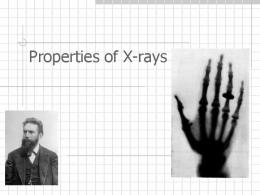
Equation (1.6) is plotted in Figure 1.3. The horizontal axis is the luminosity LX and the vertical axis is the polar cap radius r0 . Multiple curves are plotted for different electron temperatures. Electron temperatures are not expected to rise above 5 × 10⁸ K which is the hottest temperature plotted. 5
5.0
0
Te = 1e7 K 0
4.5
LMC X-4
2e7 K
Log10 HPolar Cap RadiusL
Vela X-1
CEN X-3
5e7 K
4.0
1e8 K 3.5
HER X-1
2e8 K
region for inclusive gas dynamics
3.0
5e8 K Eddington Luminosity
X-PER
2.5
2.0 33
34
35
36 Log10 HLuminosityL
37
38
39
Figure 1.3: Rough order-of-magnitude plot of the parameter space where gas dynamics is expected to play a role within the accretion column as a function of luminosity LX and polar cap radius r0 . The radiation and gas are in thermal equilibrium (blackbody) and curves are shown for various temperatures Te typically encountered in the column. To provide some perspective, the five X-ray pulsars modeled in this dissertation research are plotted in Figure 1.3. The polar cap sizes for each currently represent my best model comparisons. The dashed circle represents a rough approximation to the region in which we expect gas dynamics to be important. We call this the “region for inclusive gas dynamics”. There is no equation governing the location of this circle. It is placed on the graph such that it does not extend beyond a luminosity of 1037 erg sec−1 and does not cross an electron temperature beyond approximately 5 × 10⁸ Kelvin. A luminosity of 1037 erg sec−1 was 6
chosen because we are interested in low-luminosity sources, and certainly any luminosity higher than 1037 erg sec−1 is a high-luminosity source. We do not expect temperatures within the column to extend beyond 5 × 10⁸ Kelvin. We see that both X-PER and Vela X-1 fall within the dashed circle. Hence, gas pressure is expected to be dynamically important in these two sources. Vela X-1 roughly approximates the mid-point below which we consider pulsars as having a low luminosity. At luminosities above LX ∼ 1037 erg sec−1 we expect radiation pressure to dominate. At the top of the accretion column, boundary conditions for the incident radiation and gas Mach numbers are coupled with an improved set of hydrodynamical equations in which the bulk fluid passes through a sonic point (total Mach number equals unity). The complete dynamical solution is obtained by defining five free parameters: polar cap size r0 in units of cm, starting dimensionless accretion column height r˜start , incident radiation Mach number Mr0 , and two electron scattering cross-sections for photons traveling either parallel to (σ∥ ) to or perpendicular (σ⊥ ) the column centerline axis. Fluid bulk velocity profiles are numerically calculated and the ideal gas law is used to find the column temperature, pressure, and density as a function of distance from the stellar surface. The dynamical effects of the radiation and the ionized gas are both included in the model, which is cast in a conical geometry as a reasonable and mathematically convenient approximation to the magnetic dipole. My PhD research employs the proven finite element method to solve a new transport equation that accounts for spherical geometry rather than cylindrical geometry. This yields the photon distribution as a function of energy and height above the stellar surface. The bulk velocity profile is exact and numerically calculated. It is used instead of the Becker & Wolff approximation, and electron temperature is computed rather than assumed to be constant. All of this results in more realistic physics within the accretion column, and thus a more accurate spectra production. The emergent phase-averaged spectra is compared to data from the well-known pulsars X-PER, Vela X-1, HER-X1, CEN-X3, and LMC X-4.
7
Finally, we analyze electron scattering cross-sections for photon propagation in the transport equation to understand how changes in model parameters affect the comparison with observed data.
8
Chapter 2: An Overview of X-Ray Pulsar Observations
Nearly a half-century has passed since we began X-ray imaging our universe. The first X-ray telescope was developed in 1963 (Giacconi) and made images of hotspots in the sun’s atmosphere. Close to a decade later, in the early 1970’s, technology was improved and observations outside our solar system began with NASA’s Uhuru X-ray satellite. Since that time significant achievements and optical sensitivity improvements were made and our knowledge of X-ray sources increased dramatically. Table 2.1 is a quick look at some of the major X-ray satellites over the past four decades. The Einstein observatory, HEAO-2, was a key mission in X-ray astronomy from 1978 to 1981. It was a NASA mission which involved a consortium of scientists fromm multiple institutions, including the Harvard-Smithsonian Center for Astrophysics, Columbia University, NASA/Goddard Space Flight Center, and MIT. It had a sensitivity several one hundred times greater than any mission before it and also was the first X-ray mission to use focusing optics with imaging detectors. Einstein was responsible for lifting X-ray astronomy into the mainstream of astronomical research. EXOSAT, the European X-ray Observatory Satellite, was operational from 1983 until 1986. Its payload consisted of three instruments that produced spectra, images, and light curves in various energy bands. EXOSAT had instruments the provided improved resolution in the 1-50keV band, as well as two low-energy imaging telescopes that were sensitive in the energy range 0.05-2keV, providing the first detailed observations in the EUV band. The ROSAT satellite was a joint venture between Germany, the United Kingdom, and the United States. It was in operation from June, 1990 until it was turned off in February, 1999. At the time its telescope consisted of the largest X-ray mirrors ever built. ROSAT performed the first all-sky surveys with imaging telescopes leading to the discovery of 125,000 X-ray and 479 EUV (extreme ultraviolet) sources. 9
Table 2.1: X-ray Instrumentation Satellites and Some Significant Accomplishments. Satellite Aerobee Rocket
Country U.S.
Duration 1962
Uhuru
U.S.
1970-1973
Vela satellites
U.S.
1969-1979
Ariel V
U.K.
1975-1980
SAS-3 (Small Astronomy Satellite)
U.S.
1975-1980
High Energy Astronomy Observatory-1 (HEAO-1)
U.S.
1977-1979
Einstein X-ray Observatory
U.S.
1978-1981
EXOSAT
E.S.A.
1983-1986
Roentgen satellite
Germany
1990-1999
Advanced Satellite for Cosmology and Astrophysics (ASCA)
Japan
1993-2000
Rossi X-ray (RXTE)
U.S.
1995-Present
BeppoSAX
Italy & The Netherlands
1996-2002
Chandra X-ray Observatory
U.S.
1999-Present
XMM-Newton
E.S.A.
1999-Present
High Energy Transient Explorer (HETE-2)
U.S., Japan, France, & Italy
2000-Present
Timing
Explorer
10
Accomplishments Discovery of 1st cosmic X-ray source and the X-ray background. Discovered that neutron stars or black holes accrete matter from companion stars. Discovered gamma ray bursts and X-ray bursters. Discovered brightest X-ray source seen at the time. Discovered X-ray emission from a white dwarf star. Conducted research on wide range of X-ray energies, X-ray background, and spectra of active galactic nuclei. First X-ray telescope with mirrors. Significant scope in X-ray images, locating 7,000 X-ray sources, and brought about study of dark matter. Discovered quasi-periodic oscillations from neutron stars and black holes. Significant contributions to the study of upper atmospheres of many stars, made the first detection of radiation from the surface of neutron star. Found first evidence of gravitational redshift due to gravity field around a black hole. Detailed studies of X-ray spectra in supernova remnants. Can study rapid time variations in the emission of cosmic X-ray sources. Suggests evidence for warping of spacetime in vicinity of black holes. Scientific payload can cover three decades of energy, from 0.1 to 300 keV. High precision recording of gamma-ray bursts. Unprecented sensitivity and precision. Significant contributions and discoveries related to stars, the nature of black holes, high-energy matter and anti-matter, formation and evolution of galaxies. Detailed studies of spectra of supernova remnants, accretion disks around black holes, stars, and other sources. State-of-the-Art research on detection and localization of gamma-ray bursts.
2.1
The Beginnings of X-Ray Pulsar Research
A first investigation of the physics of accretion onto compact stars, combining the effects of stellar magnetic fields and rotation, was performed by Lamb, Pethick, and Pines (1973). In the standard model developed by these authors, accretion-powered pulsars convert kinetic energy into X-ray radiation as accreting matter flows onto the neutron star’s magnetic polar caps. Infalling matter (ionized hydrogen gas) extracted from the atmosphere of the normal companion star is channeled onto one or both magnetic caps by the strong magnetic field. Figure 2.1 shows an artist’s rendition of a neutron star accreting gaseous material from the companion star, and Figure 2.2 shows gas accretion along the magnetic field and the production of X-rays near the polar cap.
Figure 2.1: Accreting pulsar (top) and its companion star (left) form a binary star system. The pulsar attracts matter from the companion star due to its close proximity and strong gravitational pull. (NASA).
2.2
Photon Spectra and Light Curves
The magnetic poles contain “hot spots” where the extremes of the magnetic field, plasma density, and radiation transport couple together. The high temperatures in the hot spot are caused by the conversion of gravitational potential energy into kinetic energy, and then 11
Figure 2.2: Basic features of accretion onto pulsar magnetic pole are shown. To the right is a close-up view near the stellar surface. The “hot spot” near the surface produces X-rays that escape through the walls of the accretion column (Lamb, Pethick, and Pines 1973). into thermal energy at the base of the accretion column, where the matter crashes onto the surface of the star. The combination of the radiation-beaming properties of the accretion structure and the rotation of the star creates a “pulse profile” in the frame of a distant observer when the normalized amplitude of the observed flux is plotted versus the period (or phase) of rotation. These plots are also called “light curves.” Figures 2.3 and 2.4 show two light curves (White et al. 1983), the first from the lowluminosity pulsar X-PER and the second from the high-luminosity pulsar CEN X-3 (White et al. 1983). The graphs in this case are further subdivided into different energy bands, but light curves from other publications or studies might be energy-integrated such that only one curve is shown. We see that X-PER has a period of 835 seconds and a luminosity of ∼ 4 × 1033 erg sec−1 (this is equivalent to log10 [Lx ] = 33.6) shown in the upper right on the figure. CEN X-3 has a much smaller pulse period of 4.84 seconds and a higher luminosity of log10 [Lx ] = 37.9 . 1036 erg sec−1 . Lower luminosity pulsars (. 1036 erg sec−1 ) tend to show a sinusoidal-like trend in the pulse profile with a small dependence on photon energy between energy bands. At higher luminosities the pulse profiles begin to display energy dependencies. Some of the highest 12
Figure 2.3: X-PER pulse profile, a low-luminosity pulsar with a period of 835 seconds. White et al. (1982) found evidence to suggest low-luminosity pulars such as X-PER have a longer pulse period. (White et al. 1982).
13
Figure 2.4: Pulse profile for high-luminosity pulsar CEN X-3 with a period of only 4.84 seconds. The pulse shape for each energy band shows a slight change with energy. Other high-luminosity pulsars show significant profile changes with energy. (White et al. 1982).
14
Table 2.2: Some X-ray Pulsars and Associated Properties. Source (name) X-PER 4U1145-61 4U1258-61 OAO1653-40 4U0900-40 4U1223-62 4U1538-52 4U0115+63 HER X-1 CEN X-3 GX1+4 SMC X-1
Distance (kpc) 1.3±0.4 1.5 2 1.7 1.4 1.8 5.5 3.5 5 8 9 50
Pulse Period (sec) 835s 292s 272s 38s 283s 700s 529s 3.61s 1.24s 4.84s 115s 0.72s
Luminosity log10 [Lx ] 33.6 35.0 35.8 35.4-36.8 36.4 36.4 36.6 37.0 37.4 37.9 38.0 38.7
luminosity pulsars (& 1037 erg sec−1 ) even show pulse profiles with phase reversals between the energy bands. It’s important to mention that the longest pulse period pulsars tend to have the lowest luminosities (White et al. 1983). Table 2.2 shows a dozen X-ray pulsars and their associated properties. We list pulsars used in the published analysis of White et. al. (1983) and Coburn et. al. (2002). The lowest luminosity pulsars are at the top of the list and highest luminosity pulsars are at the bottom.
Figure 2.5: X-PER phase-averaged profile. (White et al. 1983).
15
Figure 2.6: CEN X-3 phase-averaged profile. The visible bump at 6-7 keV is due to an iron source emmission. The cutoff energy for CEN X-3 is approximately 11 keV where the photon count drops at a steeper decent. (White et al. 1983).
2.3
Phase-Averaged Spectra
Analysis of the X-ray spectra is often performed by averaging the pulses over many cycles and displaying these as phase-averaged (or rotation-averaged) profiles. Figures 2.5 and 2.6 show the equivalent phase-averaged spectra corresponding to X-PER and CEN X-3, respectively. Phase-averaged spectra are generally represented by a power law with energy index α, up to some high-energy cutoff location which is typically between 10 and 60 keV. The value of α is most always less than 1.0. An iron (Fe) emission feature between 6 and 7 keV is sometimes recognizable in the phase-averaged profile with equivalent widths ranging from 100 to 600 eV (White et al. 1983). The high-energy cutoff is commonly denoted by the variable Ec , and the profile shape beyond the cutoff energy is modeled by an exponential function. Coburn et al. (2002) describe in detail three analytical functions commonly used to empirically model the pulsar continuum. Although these functional forms have no physical basis, they are often used to characterize the observed spectral shapes. The first function
16
is the power law with high-energy cutoff (PLCUT):
PLCUT(E) = AE
1 −Γ
(E ≤ Ecut )
e−(E−Ecut )/Efold
(2.1)
(E > Ecut ) ,
where Γ is the photon index and Ecut and Efold are the cutoff and folding energy. The second function (Tanaka 1986) uses the same power law Γ but instead uses a Fermi-Dirac form of the high-energy cutoff (FDCO):
FDCO(E) = AE −Γ
1 1+
e(E−Ecut )/Efold
.
(2.2)
The third function (Mihara 1995) uses two power laws (Γ1 and Γ2 ) in combination with an exponential cutoff (NPEX):
NPEX(E) = A(E −Γ1 + BE +Γ2 e−E/Efold .
2.4
(2.3)
Pulse-Phase Spectroscopy
There are physical processes within the accretion column that can be easily masked if we only investigate the phase-averaged profiles, which are averaged over the pulsar spin period. Pulse-phase spectroscopy provides valuable insight into the phase-dependent spectral changes across the energy continuum observed as the pulsar spins (Serlemitsos et al. 1975; Pravdo et al. 1978). An inferred spectrum is obtained by multiplying an analytical model of the incident spectrum with a previously determined X-ray detector response matrix. We look at the spectra of the extensively studied source Hercules X-1 (HER X-1; Pravdo et al. 1977) to highlight some benefits of pulse-phase spectroscopy. Figure 2.7 shows the energy integrated (2-31 keV) pulse light curve (net counts per second) as a function of pulse phase obtained with the cosmic X-ray spectroscopy experiment (CXS) onboard the OSO 8 17
instrument. The CXS used an argon-filled proportional counter. We see the pulse shape in figure 2.7 between 2 to 30keV. There are 62 temporal bins which comprise this light curve. Pulse phase is simply an indication of the temporal evolution of the observed photon count due to the spin of the pulsar. The top graph in the figure shows a double-peaked pulse with a dominant first peak followed by a second peak. There are clearly two distinct peaks within one complete phase.
Figure 2.7: Energy integrated pulse light curve of pulsar Hercules X-1. The main pulse clearly has two distinct peaks within one complete phase (Pravdo et al. 1977). In this HER X-1 example an automatic spectral fitting program was used to obtain the best-fit parameters for a simple spectral model. The model chosen was a power law with an additional multiplicative factor of the form:
−3
spectrum ∝ e−αE ,
(2.4)
where α is a free parameter and E is the photon energy. Equation (2.4) is used as a measure of gross spectral shape. It determines the region in which the soft-to-hard spectral change occurs. 18
The parameters in the middle and bottom portions of figure 2.7 are a measure of spectral change activity. Spectral changes often occur with the temporal changes in pulse phase. In the case of HER X-1 the peak pulse intensity rises slower at higher energies. The first peak is more narrow at higher energy and also occurs at a later phase. The ‘spectral turnover’ parameter in the bottom of the figure shows relatively no spectral change activity during the main peak of the pulse profile. This is called a ‘hard region. Regions of relatively more spectral change is referred to as ‘soft’.
Figure 2.8: Pulse spectra for Hercules X-1 obtained at different pulse phases. The lower and upper curves are caused by different physical processes within the accretion column. The pulse shape arises from an energy-independent scattering process in the stellar atmosphere but the spectral changes arise from elementary processes near the stellar surface (Pravdo et al. 1977). Figure 2.8 shows two curves as a function of energy. The top curve shows the spectra from a single temporal bin within the hardened region of the pulse shape. The bottom curve is the spectra analyzed from a time bin in the region between the two pulse peaks. This clearly shows an uneven relationship between intensity and spectral changes in the pulse. Overall the energy-integrated pulse shape results from energy-independent scattering processes in the stellar atmosphere, while the spectral changes arise from processes near the stellar surface (Pravdo et al. 1977). A second example of pulse phase spectroscopy comes from the source CENTAURUS X-3 (CEN X-3). The pulse profile is shown in figure 2.4 and the spectra is shown in figure 19
2.9. Here we see the incident spectra of CEN X-3 at three different pulse phases: centered on the principal peak (P), the interpulse (I), and pulse minimum(L). You can clearly see the iron line emission in the pulse minimum spectra.
Figure 2.9: Pulse spectra for CEN X-3 at three different phases centered on the principal peak (P), the interpulse (I), and pulse minimum (L). (White et al. 1982). Recent work by Coburn et al. (2002) analyzed how cyclotron resonance scattering features (CRSFs) correlate with the shape of the pulse spectra (also called “cyclotron lines”). The line-like spectral features arise as a result of the scattering of photons by electrons with quantized energy levels (Landau levels) due to the pulsar’s magnetic field (M´ esz´ aros 1992). CRSF widths are roughly proportional to their energy and provide insight into the magnetic field strength. Coburn et al. (2002) also showed a correlation between magnetic field strength and the spectral cutoff energy. In the next chapter we will briefly discuss work by Becker and Wolff (2005, 2007b) which eliminates the need to phenomenologically model the high-energy cutoff region using empirical fitting functions such as those in equations (2.1), (2.3), and (2.2). They provided the first physically motivated calculation of the spectrum which accurately reproduces the power-law variation commonly seen in many accreting X-ray pulsar spectra. 20
Chapter 3: Current Theory of Accretion Column Formation
In this chapter we review the current dynamical theory of accretion columnn formation. Drawing upon ideas presented by Lamb, Pethick, and Pines (1973), Davidson (1973), Basko & Sunyaev (1975, 1976), and Wang & Frank (1981), we follow the concepts used to describe the structure of pulsar accretion column formation in modern theories by Becker (1998), Bykov & Krassilchtchikov (2004), and Canalle et. al. (2005). The current dynamical theories of accretion column formation focus exclusively on either radiation-dominated flows or gas-dominated flows, in which the gas is composed of ions and electrons in a fully ionized plasma. However, none of the current models implement a twofluid concept whereby gas and radiation fluids are mutually considered. The Becker (1998) model focuses exclusively on radiation-dominated flows with a standing, radiative shock. Both the Canalle et al. (2005) and Bykov & Krassilchtchikov (2004) models investigate accretion dynamics of a plasma fluid with a quasi-stationary shock. Canalle et al. (2005) apply an accreting, single-fluid model to the post-shock region only and the region above the shock only establishes an upper boundary condition. Bykov & Krassilchtchikov (2004) investigate a two-component model of ions and electrons which have the same bulk velocity but different temperatures along the column. My PhD research implements a never-before considered two-fluid model in which the pressure is provided by both the gas and the radiation. All of the previously published dynamical models show that a shock is present in the accretion column, whether stationary or quasi-stationary, as the inflowing material slows before approaching the stellar surface. A shock must occur in pulsar accretion columns since the material starts out with a highly supersonic velocity (close to the speed of light), and it essentially comes to rest at the stellar surface. The shock compression ratio, however, varies 21
in the different models. Canalle et al. (2005) assume that the upstream Mach number tends to infinity and use the Rankine-Hugoniot condition to derive the post-shock velocity, which is equal to precisely
1 4
of the pre-shock velocity. The Bykov & Krassilchtchikov (2004)
model uses the well-known Godunov method to investigate the shock discontinuity, and their numerical results show a similar compression ratio of approximately
1 4.
Neither of
these models provides an adequate description of accretion onto an X-ray pulsar since the material must come to rest in the downstream region. The Becker (1998) model implements a radiation-dominated shock which must be radiative in nature in order to convert the kinetic energy of the infalling gas into radiation such that the accreting material (considered as an ideal fluid) can come to rest at the stellar surface. The radiative shock is a continuous velocity transition and possesses a definite sonic surface profile as shown in Figure 3.1. The shock plays a crucial role in photon energization via the first-order Fermi energization process. The first-order Fermi energization process is the process whereby the accreting background plasma gas will compress and perform P dV work on the radiation, thereby transferring an energy gain to the photons. The inflow speed of the accreting electrons is much higher than their thermal velocity, and this dominates the energy spectrum dynamics except at the higher energy bands. Previous models studying radiative pulsar accretion flow neglected the role of the shock in upscattering the radiation and forming the emitted spectrum. This makes the Becker model an attractive prime candidate for further scientific inquiry. All the model geometries are simplified for ease of analysis and physical interpretation. Whereas Becker uses a one-dimensional, plane parallel geometry, both Bykov & Krassilchtchikov and Canalle et al. implement a curvilinear coordinate system which is natural for the dipole-field geometry of the magnetic field lines. In the hydrodynamic equations, however, all three models adopt a one-dimensional velocity of highly constrained flow along the field lines due to the large magnetic field strengths of X-ray pulsars. We expect that in high-luminosity X-ray pulsars the radiation pressure dominates over gas pressure (Prad ≫ Pgas ). Becker used this approach in which the pulsar luminosity LX 22
Figure 3.1: Infalling gas (fully-ionized hydrogen) passes through a radiation-dominated, standing shock while coming to rest at the stellar surface. (Becker & Wolff 2007). satisfies the constraint LX & Lcrit such that the accreting gas passes through a radiationdominated, standing shock and comes to rest (stagnates) at the stellar surface. Lcrit is given by (Becker 1998; Basko & Sunyaev 1976):
Lcrit ≡
2.72 × 1037 σT M∗ r0 , erg sec−1 √ σ⊥ σ ∥ M⊙ R∗
(3.1)
where M∗ is the stellar mass, R∗ is the stellar radius, r0 is the polar cap radius (we assume a cylindrical geometry such that it is also the radius of the accretion column), σT is the Thomson scattering cross section, and σ∥ and σ⊥ define mean values for the electron scattering cross-sections for photons radiating parallel and perpendicular to the magnetic field, respectively. Equation (3.1) gives the relationship between the luminosity LX and mass accretion rate M˙ : LX =
GM∗ M˙ , R∗
23
(3.2)
where M˙ is related to the mass flux J using:
M˙ = πr02 J
(3.3)
for a polar cap with radius r0 . In the Becker (1998) dynamical solution for bulk flow, a unique relationship exists between the luminosity LX and mass flux J for a radiation dominated flow which satisfies bulk stagnation at the stellar surface. Using equation (5.5) from Becker (1998) for the mass flow rate M˙ and substituting into equation (3.2) we obtain equation (3.1). This is applicable for a strong shock where the incident radiation Mach number is expected to be large. Becker also showed that high-luminosity pulsars have high accretion mass flow rates in which the flux exceeds the Eddington flux by roughly two orders of magnitude (∼100). The Eddington flux is the inflowing mass flux of the plasma gas at which point the force of gravity acting upon an average electron-proton couplet is exactly offset by the momentum transferred to the couplet via radiation scattering. In X-ray pulsar accretion flows, the inflowing plasma is funneled onto the small polar cap by the super-strong magnetic field. The magnetic field pressure far exceeds the radiation, gas, and ram pressures of the fluid as it moves towards the polar cap. To show an order-of-magnitude comparison between these pressures, we assume that the accretion column is in thermal equilibrium at a constant temperature Te . Radiation pressure is given by the Stefan-Boltzmann law:
1 Pr = aTe4 , 3
(3.4)
where a = 7.56 × 10⁻¹⁵ erg cm−3 deg−4 . Gas pressure is given by the ideal gas law:
Pg = ni,e kTe ,
(3.5)
where ni,e = ni = ne is the number density of electrons and ions, k is Boltzmann’s constant,
24
and Te is the electron temperature. The kinetic ram pressure of the bulk fluid is given by:
1 Pram = ρv 2 , 2
(3.6)
where v is the bulk fluid speed and ρ is the mass density. We approximate the bulk fluid speed using the free-fall velocity: vff2 =
2GM∗ , R∗
(3.7)
where M∗ and R∗ are the stellar mass and radius, respectively. Finally, for a magnetic field of strength B the magnetic field pressure is given by:
Pmagnetic =
B2 . 8π
(3.8)
To obtain typical values for the temperature and mass density we refer to Figure 4.1. We choose a temperature of Te = 108 K, a mass density of ρ = 100 g cm−3 for approximately the maximum values we expect to encounter within the accretion column. We choose a magnetic field strength of Bfield = 1012 G as a conservative value. Using these values in equations (3.4)-(3.8) we obtain the values for typical pressures. These are summarized in Table 3.1. We see that, using the values listed in this paragraph, the magnetic field pressure is stronger than all other pressures by a factor of nearly 106 . In this situation the magnetic field pressure will have a tight hold on the plasma gas and confine it to the accretion column. The ions and electrons will not escape. The inflowing gas scatters the radiation and causes it to diffuse out the side walls of the accretion column rather than propagate upstream. A “fan” beam pattern emerges rather than a vertical “pencil” pattern. In contrast to this, however, sub-Eddington pulsars have lower mass flow rates that result in lower-luminosity and in these sources, the ordinary gas component has much more influence upon the overall dynamic pressure within the accretion column. The Bykov & Krassilchtchikov (2004) and Canalle et al. (2005) models adopt the 25
Table 3.1: Pressures Expected within Accretion Column Pressure Type Blackbody
Abbreviation Pr =
Magnitude 2.52 ×
(1/3)aTe4
Relative Strength
1017
6.3 × 10⁻⁶
Gas
Pg = ni,e kTe
8.25 × 10¹⁵
2.1 × 10⁻⁷
Ram (kinetic)
Pram = (1/2)ρv 2
1.80 × 10¹⁶
4.5 × 10⁻⁷
Magnetic field
Pmagnetic = B 2 /8π
3.98 × 10²²
1
sub-Eddington approach of gas dominated flows and neglect the radiation fluid. Instead, both models incorporate upper boundary conditions in which the accreting material is considered to be a cold, supersonic, free-falling gas. Common to all three models is the implementation of hydrodynamic conservation equations. We mentioned earlier that Bykov & Krassilchtchikov and Canalle et al. consider dipole geometry in one dimension along the field lines. We look at the Becker model here and discuss where the other models deviate. Becker adopts a one-dimensional, steady-state cylindrical geometry where the conservation equations of mass, momentum, and energy are given by:
∂ ∂t
(
1 2 ρv + Uradiation 2
∂ρ ∂J =− =0 ∂t ∂x
(3.9)
∂ ∂I (ρv) = − =0 ∂t ∂x
(3.10)
) =−
∂E + U˙ escape + U˙ absorbed + U˙ emitted = 0, ∂x
(3.11)
where the x variable describes the spatial dimension directed towards the stellar surface. The variables J, I, and E represent the fluxes for mass, momentum, and total energy, respectively. Uradiation is the internal energy density of the radiation and the U˙ terms on the right-hand-side of equation 3.11 represent the rate of change of internal radiation energy density due to radiation escape from the accretion column walls, photon absorption by the gas within the column, and photons emitted by the gas, respectively. Mathematically the
26
fluxes are represented by the following expressions:
J = ρv
(3.12)
I = P + ρv 2
(3.13)
1 ∂P E = ρv 3 + P v + U v − c , 2 ∂τ∥
(3.14)
where P, U, ρ, and v are the fluid radiation pressure, internal energy density, mass density, and flow velocity, respectively. The speed of light is given by c. The optical depth τ∥ is related to the spatial dimension using
dτ∥ = ne σ∥ dx,
(3.15)
where the local electron density ne is a function of height above the stellar surface and plays an important role in the diffusion of the radiation energy along the accretion column axis. An important assumption made is that the flow is optically thick to electron scattering perpendicular to the flow direction. We use the diffusion term in equation (3.14) to model the escaping radiation flux Frad : Frad = −c
∂P . ∂τ∥
(3.16)
To investigate equation (3.16) we convert the optical depth to the spatial domain using equation (3.15) to obtain: Frad = −
c ∂P . ne σ∥ ∂r
(3.17)
The quantity c/(ne σ∥ ) has units of cm2 sec−1 and is the diffusion coefficient for radiation traveling parallel to the accretion column axis. Therefore, as the radiation moves towards the stellar surface the radiation pressure will increase and cause a spatial gradient. The
27
gradient multiplied by the diffusion coefficient yields the energy flux. This provides the mechanism for the formation of a radiative shock which drives the very important firstorder Fermi energization of photons. The approach of Wang & Frank (1981) is used in which constant, energy-averaged electron scattering cross sections σ∥ and σ⊥ describe the scattering of photons propagating parallel and perpendicular to the column magnetic field, respectively. The Becker model (1998) is unique because it applies a diffusion approximation to the energy flux that effectively models the radiative nature of the standing shock. In this model, the energy flux E decreases as the gas approaches the stellar surface due to the escape of radiation energy through the walls of the accretion column. There are important physical effects, however, not included by Becker (1998). These include gravity, bremsstrahlung radiation production and re-absorption losses, and cyclotron radiation emission. The Canalle et al. (2005) model implements gravity effects in addition to a cooling function with a power-law dependence on density and temperature. This cooling function allows for a crude investigation of flow dynamics for bremsstrahlung and cyclotron losses. The Bykov & Krassilchtchikov model (2004) includes bremsstrahlung and cyclotron cooling losses, and they also add corrections for effective forces acting on the ions and electrons, which include gravity, radiative pressure, and friction forces in the atmosphere. Continuing our review of Becker’s model, we can reasonably assume in equation (3.11) that U˙ absorbed + U˙ emitted ≈ 0 because the fluid is radiation-dominated and any energy supplied to the radiation field is supplied by the photons themselves. In this case the energy insertion processes of thermal Comptonization, bremsstrahlung heating, or cyclotron heating can alter the shape of the spectra but they do not result in a net change in internal energy. My PhD research considers new dynamics in which bremsstrahlung and cyclotron emission production and absorption losses play a major role in the accretion column dynamical structure. The relationship between internal energy density and pressure is given
28
by: U=
P , γrad − 1
(3.18)
where the value for the specific heat ratio (adiabatic index for radiation) is given the constant value γrad = 4/3. Steady-state solutions are sought such that time-dependent terms can be eliminated. Although the Bykov & Krassilchtchikov model solves time-dependent equations, their solution quickly converges to a static condition that we can use to compare against the Becker solution. The Canalle et al. model solves for steady-state solutions as well. Returning to the Becker model, the desired steady-state conditions permit the mass and momentum fluxes to be conserved, but the energy flux decreases as the fluid approaches the stellar surface due to the energy escaping through the column walls via the rate of energy escape term U˙ esc in (3.14). These conditions led Becker to arrive at the important dynamical equation that governs the flow structure:
d dτ
(
7 dµ − µ2 + 7µ + 2 dτ
)
( = −3θξ µ
2 2
) 7 −µ , 4
(3.19)
where µ and τ are dimensionless parameters defined as:
µ≡
v vc , τ ≡ τ∥ , vc c
(3.20)
and vc is the critical velocity, which is the flow velocity at the sonic point. The sonic point is the height in the column where the Mach number with respect to the radiation sound speed equals unity (M = 1). The variable ξ is defined as the loss parameter:
ξ2 ≡
mp 2 c2 , r0 2 J 2 σ ⊥ σ ∥ 29
(3.21)
which describes the strength of energy loss due to the radiation escaping across the accretion column outer walls. The variable θ is called the transparency function and is approximated as θ(τ ) ∼ 1 in the space between the sonic point and the stellar surface. This corresponds to radiative flow downstream of the sonic point. Setting θ = 0 would result in purely adiabatic flow with no radiative losses. mp is the proton mass and r0 is the polar cap radius. The downstream boundary conditions are crucial to understanding the physics at the stellar surface. We follow the approach first considered by Davidson (1973) and Basko & Sunyaev (1975, 1976) to maintain the requirement of a fluid stagnation boundary condition. All three of the newer models require stagnation at the stellar surface. These provide a simple and plausible explanation for the behavior of the fluid velocity below the shock transition. Bykov & Krassilchtchikov require stagnation but their model shows that a positive stellar surface energy flux remains. I later show in my research that the bulk fluid velocity does not necessarily stagnate. My HER-X1 dynamic solution shows a small residual velocity remains at the stellar surface, and the CEN-X3 solution shows an even larger bulk velocity remains. We take a closer look now at the stellar surface boundary condition that requires a radiative, stagnating flow. After passing through the shock the matter accumulates on the polar cap to such great extent that mathematically we have:
lim Massacc (x) → ∞,
x→xst
(3.22)
where Macc is the mass inside the accretion column. Using the relationship given in equation (3.15) the parallel scattering optical depth at the stellar surface is also:
lim τ∥ (x) → ∞,
x→xst
(3.23)
and it can be shown that as τ∥ → ∞ the total energy flux vanishes at the surface of the star (not accounting for the energy flux associated with gravity) which leads to the additional 30
downstream boundary condition of
lim E(τ ) → 0.
(3.24)
τ∥ →∞
This is called the “mirror condition”. The requirement of stagnation at the stellar surface leads to an eigenvalue condition for the loss parameter ξ, yielding the specific value ξ 2 = (8/3)ϵc . Solving equation (3.19) yields the fluid velocity profile and the shock location relative to the stellar surface: ( µ(τ ) =
7 2ϵc + 7
)(
[ 1 − tanh
where: 2 τ∗ ≡ tanh−1 7
(
]) 7 (τ − τ∗ ) , 2
) 2 ϵc . 7
(3.25)
(3.26)
A precise form of the transparency function θ(τ ) is chosen such that downstream θ ≈ 1 between the sonic point and stellar surface, and θ → 0 in the upstream region where the flow is assumed to be adiabatic. Becker (1998) adopted the form:
1 θ(τ ) = 2
{ [ ( ( ))]} 7 2 −1 2ϵc − 4 1 + tanh τ − tanh 2 7 3
(3.27)
where ϵc is the dimensionless energy flux at the sonic point:
ϵc ≡
E , Jvc2 τ =0
(3.28)
where τ was established to be zero at the sonic point. We convert from energy flux to the
31
incident (upstream) mach number M∞ via the relationship √ M∞ =
6 , 2ϵc − 1
(3.29)
which will allow us to use M∞ as a free input parameter. This relationship was obtained by allowing τ → −∞ at the far upstream location (essentially adiabatic flow) and combining the dynamic solution for µ(τ ) with the relationship between Mach number and µ. Becker (1998) provides more detail on these equations.
Figure 3.2: Analytical solution of dynamical equation (3.19) showing velocity ratio µ ≡ v/vc and the transparency function θ(τ ) plotted as a function of the scaled scattering optical depth τ (Becker 1998). The incident mach numbers for the solid and dashed lines are M∞ = 10 and M∞ = 2.45, respectively. The transparency function initially is zero and increases to almost unity at the critical point (τ = 0). Far upstream the incident velocity is greater than the critical velocity (τ < 0), is equal to critical velocity at τ = 0, and stagnates at the stellar surface near τ = 1.0 (Becker 1998). In the limiting case of a strong shock where M∞ → ∞ we see that ϵc →
1 2
and ξ 2 →
4 3
(Becker 1998; Basko & Sunyaev 1976). Using this result and converting to x coordinates we arrive at the exact analytical solution for fluid velocity along the column: [ ( )−1+x/xst ] 7 7 v(x) = 1− vc , 4 3
(3.30)
where the quantity xst defines the distance between the sonic point and the stellar surface 32
and is given by (Becker 1998)
r0 xst = √ 2 3
(
σ⊥ σ∥
)1/2
( ) 7 ln . 3
(3.31)
Figure 3.2 shows the numerical solution to the dynamical equation for the Becker model. The incident mach numbers for the solid and dashed lines are M∞ = 10 and M∞ = 2.45, respectively. The sonic point is located at τ = 0. The two sets of curves show the values of the variable µ(τ ) and the transparency function θ(τ ). Far upstream (τ = −1.5) the value of µ is greater than unity because the incident velocity is greater than the critical velocity µ ≡ v/vc > 1, whereas the transparency function is zero. As the flow approaches the critical point (τ = 0) the theta function approaches unity, and the velocity equals the critical velocity such that µ = 1. The fluid stagnates at the stellar surface and the transparency function θ(τ ) is closely equal to unity between the sonic point and the surface. This solution provides an accurate description of the flow structure between the sonic point and the stellar surface for cylindrical geometry. The Canalle et al. (2005) model investigates flow only in the post-shock region in contrast to a numerical analysis along the full column length. This is a disadvantage because an assumption about the shock strength must be made prior to solving the problem, and the solution will not provide a fluid velocity profile upstream of the shock. Aside from this, Canalle et al. found that the dipolar geometry of the problem resulted in proportionally higher pressures throughout the post-shock region as compared to a purely cylindricalgeometry model of Cropper et al. (1999). See figure 3.3. Canalle et al. also noticed that compressional heating due to the dipolar geometry was as important as radiative cooling and gravity in determining the structure of the post-shock flow in accreting white-dwarf stars. Bykov & Krassilchtchikov (2004) perform a time-dependent numerical analysis along the entire column length up to several star radii from the stellar surface. They model the
33
Figure 3.3: Post-shock pressure profiles of Canalle model (2005) in both cylindrical and dipole coordinates. The horizontal axis shows distance above the stellar surface. The stellar surface is at (r − 1)/(rs − 1) = 0 on the left and the radiation shock is at (r − 1)/(rs − 1) = 1 on the far right. The pressure for dipole geometry is proportionally higher than the purely cylindrical coordinates. one-dimensional motion of the accreting plasma along the magnetic field dipole lines. Their equations are integrated from an initial state at t = 0 to a current state at a moment t in a number of time steps ∆t. Their results show that a strong, collisionless shock evolves in about 10−5 seconds. After several free-fall periods a quasi-stationary state of the column with a stable accretion shock is usually reached. They also discovered that the accretion dynamics significantly depend on the detailed structure of the magnetic fields about 103 cm from the surface. The Becker model provides the first steps towards a complete, self-consistent description for both the shock dynamical structure and the radiative transfer in the column. However, the resulting velocity profile does not incorporate the effects of the gas pressure, the strong gravitational field, or the dipole structure of the column.
34
Chapter 4: The Physics of X-Ray Spectra Formation
Until recently, attempts to calculate the spectra of accretion-powered X-ray pulsars usually did not yield good agreement with the observed spectra. This lack of agreement reflects the phenomenological nature of the methods that were employed in those efforts. In this chapter, I review the current state of the field and describe the methods used in the dissertation to calculate the spectra of X-ray pulsars based on the detailed microphysics occurring in the accretion columns.
4.1
Radiation Hydrodynamics
The intent of this section is to review the fundamentals of radiation transport and to investigate the validity of the diffusion approximation employed in the dissertation research. The radiation field can be described by either a photon distribution function f or the spectral radiation intensity Iν . The intensity has units of erg sec−1 cm−2 sr−1 ν −1 . We say the intensity is the energy crossing a unit area at a given point per unit time per unit frequency and per unit solid angle in the direction of interest. A distribution function f captures the concept of the particle nature of radiation where we introduce the concept of the quanta. Each quanta has an energy hν. The phase space density f is related to the intensity Iν by the following: f=
Iν dN 3 = h4 ν 3 /c2 , dV d p
(4.1)
where the momentum space volume element, in spherical momentum-space coordinates, is: ( )3 h ν 2 dνdΩ. d p= c 3
35
(4.2)
The key ingredient that makes this relationship possible is that a quanta has an energy hν and a momentum hν/c. From equation (4.1) we see the units of the phase space density function are the total number of photons N per a volume element V per differential photon momentum space. The quantum nature of the photon allows us to work with either function and easily switch to the other. In our application the radiation transport equation can be written as: 1 ∂Iν + n · ∇Iν = jν − kν Iν , c ∂t
(4.3)
where Iν is the intensity (erg sec−1 cm−2 sr−1 ν −1 ), jν is the emission coefficient (erg sec−1 cm−3 sr−1 ν −1 ), kν is the scattering coefficient (cm−1 ), and n represents a unit vector which points in the direction of radiation propagation. The emission coefficient and scattering coefficient describe the interaction of radiation and matter. Energy is either (1) removed from matter and added to the radiation (via the jν emission term), or (2) energy is scattered by matter and removed from the radiation (via the −kν Iν scattering term). The presence of the unit vector n indicates the intensity has a directional dependence. We are going to replace the direction-dependent intensity in the radiative transport equation with the angle-averaged distribution function which directly governs the spectral energy density and energy flux. By using the distribution function the angular distribution of the radiation is not present when considering the radiation interaction with the bulk fluid. The diffusion approximation greatly simplifies solving equation (4.3). In our application the approximation is accurate when the photon scattering mean free paths are small compared to other length scales. Mathematically we can write this as:
kν L ≫ 1,
(4.4)
where L is a typical length in the problem and here kν refers to a scattering coefficient. This is simply the optical depth τ and describes a probability per unit length kν that a photon will scatter with matter as it traverses some thickness L. An optically thick medium
36
(τ ≥ 1) is one in which the average photon of frequency ν cannot traverse the entire medium without being scattered. The scattering mean free path (1/kν ) is small and the radiation density should change little over this distance. We can consider the radiation field for such small gradients to be almost isotropic. The diffusion approximation is an expansion in the scattering mean free path (1/kν ) in which successive approximations for obtaining Iν are terminated after the first two terms. We use the assumption that kν is large (scattering mean free path is small) and has a very small correction to the first term. The the diffusion approximation equation is written as:
jν 1 Iν = − kν kν
(
1 ∂jν /kν jν +n·∇ c ∂t kν
) .
(4.5)
There is no need to find additional approximations because we are assuming kν is large and the next term would be negligible. We obtain additional properties from the intensity by taking its angle moments. The angle θ described here represents the angular distance from the normal vector n to some differential amount of flux from the solid angle dΩ. The first moment of equation (4.5) yields the proper energy flux in the diffusion approximation. The differential energy flux is equal to: dFν = Iν cosθ dΩ ∝ erg s−1 cm−2 Hz−1 ,
(4.6)
which represents the energy crossing a unit area of a detector per unit time due to a beam of radiation making an angle θ with respect to the detector. The total energy flux is therefore given by: ∫ Fν =
∫ dFν =
Iν cos θdΩ ∝ erg s−1 cm−2 Hz−1 ,
(4.7)
where the bounds of integration cover the angle subtended by the source at the detector.
37
The total energy density is likewise given by: ∫ Uν =
∫ dUν =
1 Iν dΩ ∝ erg cm−3 Hz−1 , c
(4.8)
We relate the phase space density function f to the energy density Uν by substituting equation (4.1) into equation (4.8) to obtain: ∫ Uν =
∫ dUν =
h4 ν 3 f dΩ. c3
(4.9)
Finally, the second moment in the diffusion approximation yields the pressure and is found by multiplying by nn and integrating over all angles. In one dimension we obtain: ∫ Pν
=
nn Iν dΩ
(4.10)
=
[ ( )] 4π ∂ jν 1 4π jν − 3 c kν kν c2 ∂t kν
(4.11)
=
1 Uν . 3
(4.12)
We see that by using the diffusion approximation the Eddington approximation in equation (4.12) follows.
4.2
Justification for the Ideal Gas
An essential element in the modeling of structure in the accretion column is the Equationof-State (EOS) that describes in precise mathematics how the pressure of matter responds to changes in its density and temperature. Figure 4.1 shows a temperature-density log-log plot of the regions which are governed by different equations of state (H. Bradt, Asrophysics Processes, Cambridge University Press 2008). The boundaries between the several regions 38
are lines of equal pressure. Our research is limited to nondegenerate material in the upper left quadrant of the graph in which the column temperature is sufficiently high (∼ 106 108 K) and the density is low (ρ ∼ 10−4 -100 g cm−3 ). We neglect any effects from electron degeneracy and quantum mechanics throughout this research because the densities are low enough and the temperatures are high enough such that classical Maxwell-Boltzmann statistics apply.
Figure 4.1: A temperature-density log-log plot shows the regions where different equations of state apply. The boundaries between the several regions are lines of equal pressures. Our research is limited to the upper-left quadrant of the plot which is governed by nondegenerate matter. (H. Bradt, Asrophysics Processes, Cambridge University Press 2008) The ionized plasma gas (hydrogen) we are investigating has a temperature Te which contains particles traveling in random directions with a wide range of speeds. We can rightfully suppose the gas is in thermal equilibrium because collisions allow the energy to be equally shared among all the particles. The ionized gas has interparticle forces (electrostatic interaction between the electrons and protons) but their potential energies are an 39
order of magnitude less than the kinetic energy density. The Maxwell-Boltzmann (MB) distribution is perfectly suited for such a scenario in which the gas is comprised of pointlike and nonrelativistic particles with negligible interparticle forces. As long as the ionized gas interaction energies are small compared with their kinetic energies we shall use the equation of state of a perfect gas to describe the radiation and gas fluids. The physical form of our equation of state is:
P =
R ρT. µ
(4.13)
This can be re-written as: P = (γ − 1)ρe.
(4.14)
where γ = cp /cV is the ratio of specific heats. The quantity ρe is the internal energy density U . When γ = 4/3 we obtain for radiation:
1 Pr = Ur . 3
(4.15)
This establishes that the radiation can be treated as an ideal gas with γ = 4/3. However, we can only assign a temperature to the radiation field if it is in full thermodynamic equilibrium with the matter, which probably occurs close to the bottom of a pulsar accretion column.
4.3
Becker & Wolff Model
A new model for X-ray spectral formation was recently developed by Becker and Wolff (2005a, 2005b) based upon the “bulk” Comptonization (i.e., the first-order Fermi energization) of photons due to the convergence of the gas in the accretion column. A first-order Fermi term is included in the transport equation which accounts for the transfer of proton kinetic energy to the photons via electron scattering as the photons travel back and forth across the accretion shock. Thermal Comptonization was ignored in their “bulk” model, 40
and as a result the computed X-ray spectrum contained no high-energy cutoff. Not including the effects of thermal Comptonization corresponds physically to a “cold plasma” in which the thermal velocity of the electrons is much less than the dynamical (bulk) velocity. Becker and Wolff were successfully able to reproduce the observed spectra of several sources using the pure bulk Comptonization model. Figure 4.2 shows the count rate spectrum of X-ray pulsar 4U 1258-61 which is in good agreement with the Becker & Wolff numerical solution.
Figure 4.2: Numerical solution of Becker & Wolff bulk Comptonization model (2005a, 2005b) for column-integrated count rate spectrum of X-ray Pulsar 4U 1258-61. The solid, dashed, and dot-dashed lines correspond to accretion column densities of NH = 0, 3 × 10²¹ , and 9×1021 cm−2 , respectively. The pulsar spectrum does not have a high-energy cutoff. In this case the first-order Fermi energization process dominates the energy exchange between the electrons and photons. (Becker & Wolff 2005). However, many bright X-ray pulsars have a high-energy quasi-exponential cutoff at ∼2030 keV which suggests there is another physical process that must be taken into account besides pure bulk Comptonization. This can be explained as a result of thermal Comptonization. Thermal Comptonization is a two-step process in which high-frequency photons lose energy to electrons via Compton scattering and subsequently the low-frequency photons gain energy via inverse Compton scattering. The thermal process is described mathematically by the Kompaneets (1957) equation. Becker & Wolff (2007) extended their original model to account for this.
41
4.3.1
Photon Transport Equation
Bulk and thermal Comptonization effects are included in a transport equation used to model the production of the emergent radiation spectrum (Becker & Wolff 2007). Source photons (also called “seed” photons) are introduced into the accretion column via Bremsstrahlung, Cyclotron, and blackbody processes. Bremsstrahlung and Cyclotron photons are introduced throughout the length of the column whereas blackbody radiation is produced only at the thermal mound surface. The source photons scatter with electrons, diffuse throughout the accretion column, and eventually escape through the column walls to produce the observed X-ray spectrum. We introduce the time independent, flux-conservation form f (z, ϵ) of the photon distribution function (Gleeson & Axford 1967; Skilling 1975; Becker 1992):
∂f 1 ∂ = 0 = −∇ · Fparticle + 2 ∂t ϵ ∂ϵ
( ϵ2 D
−
∂f ∂ϵ
) −
) 1 ∂ ( 2 ϵ ⟨ ϵ⟩ ˙ f loss ϵ2 ∂ϵ
] 1 ∂ [ 2 ϵ (ϵ⃗ v · ∇f ) + f˙source − f˙escape − f˙abs , (4.16) 3ϵ2 ∂ϵ
where v < 0 to indicate that bulk velocity is towards the stellar surface. The specific particle flux Fparticle (where the “particles” are photons) is given by:
Fparticle = −κ∇f −
⃗v ϵ ∂f . 3 ∂ϵ
(4.17)
The phase-space density of photons is represented by f , ϵ is the photon energy, D is the momentum diffusion coefficient given by:
D=
ne σ ¯ c kTe , me c2 ϵ2
42
(4.18)
the momentum loss rate ⟨ϵ⟩ ˙ loss is:
⟨ϵ⟩ ˙ loss = −
ne σ ¯c 2 ϵ , me c2
(4.19)
and the f˙ terms represent the rate of change of the phase-space density due to photon source production, escape, and absorption. When we combine equations (4.16) through (4.17) and implement cylindrical, planeparallel geometry we obtain a photon distribution function f (z, ϵ) which satisfies the transport equation (Becker & Begelman 1986; Blandford & Payne 1981a; Becker 2003):
∂f dv ϵ ∂f ∂ ∂f +v = + ∂t ∂z dz 3 ∂ϵ ∂z
(
c ∂f 3ne σ∥ ∂z
) −
f tesc
[ ( )] ne σc 1 ∂ 4 ∂f Q(z, ϵ) + ϵ f + kTe + , (4.20) 2 2 me c ϵ ∂ϵ ∂ϵ πr0 2
where f is normalized such that ϵ2 f (z, ϵ)dϵ gives the number density of photons in the energy range between ϵ and ϵ + dϵ. The f˙abs term is not included here because bremsstrahlung absorption was not included in the Becker & Wolff (2007) cylindrical model. The z coordinate is used to describe the distance from the stellar surface (where the stellar surface is located at z = 0). The photon source function Q(z, ϵ) is also normalized so that ϵ2 Q(z, ϵ)dϵdz gives the number of seed photons injected into the accretion column per unit time between column height z and z + dz with energy between ϵ and ϵ + dϵ. The various terms in the transport equation contribute to f as follows: • Comoving time derivative: ∂f ∂f f˙advection = +v . ∂t ∂z
43
(4.21)
• First-order Fermi energization of the electrons (the “bulk” Comptonization):
dv ϵ ∂f f˙bulk Comptonization = . dz 3 ∂ϵ
(4.22)
• Spatial diffusion along the accretion column axis:
∂ f˙diffusion = ∂z
(
c ∂f 3ne σ∥ ∂z
) .
(4.23)
• Photon escape through the column walls:
f . f˙escape = tesc
(4.24)
• Thermal Comptonization through application of the Kompaneets (1957) operator: [ ( )] ∂f ne σc 1 ∂ 4 ϵ f + kT . f˙Kompaneets = e me c2 ϵ2 ∂ϵ ∂ϵ
(4.25)
This equation was first published in 1956 by the Soviet physicist Aleksander Kompaneets. It describes the time rate of change of the photon distribution function (the evolution of the spectrum) due to Compton scattering, or Comptonization. The first term in equation (4.25) represents the rate of change of f due to energy transferred from photons to electrons in the Comptonization process, also known as the “recoil effect” in which the radiation is “cooled” and the photon wavelength increases on scattering from electrons. The second term in equation (4.25) represents the rate of change in f due to the statistical increase of energy (“heating”) of the photons by hotter electrons which corresponds to a diffusion in photon phase space. In a perfectly thermalized environment the gas and radiation are in equilibrium and the Kompaneets 44
contribution to the transport equation (4.20) is zero. • Photon source term for the production of seed radiation throughout the column. This term includes the primary sources of seed photons from Bremsstrahlung and Cyclotron emission, as well as blackbody radiation at the thermal mound (Arons et al. 1987):
Q(z, ϵ) f˙sources = . πr0 2
(4.26)
Following the approximation given by Wang & Frank (1981), Becker & Wolff approximate the mean scattering cross section for photons propagating parallel and perpendicular to the field as follows: ( σ∥ ≈ σT
ϵ ϵc
)2 ,
(4.27)
and σ⊥ ≈ σ T ,
(4.28)
where ϵ is the mean photon energy and ϵc is the Cyclotron energy. However, a problem arises with finding the value for the mean photon energy because the radiative transfer problem must be solved before its value can be calculated. A work-around to this problem is to use the loss parameter in (3.21) to redefine the parallel scattering cross-section as ( σ∥ =
πr0 mp c M˙ ξ
)2
1 . σ⊥
(4.29)
The third and final scattering cross-section appearing in the transport equation is the angle-averaged cross section σ ¯ . Becker & Wolff verified that σ∥ ≪ σ ¯ ≪ σ⊥ as they developed their numerical model. This is in good agreement with the expected values (Canuto et al. 1971). The approach used by Becker & Wolff (2007) for solving the transport equation is to 45
obtain the Green’s function fG (z0 , z, ϵ0 , ϵ) and then calculate the particular solution for the spectrum f (z, ϵ) associated with an arbitrary photon source Q(z, ϵ) using the integral convolution (Becker 2003) ∫
∞∫ ∞
f (z, ϵ) = 0
0
fG (z0 , z, ϵ0 , ϵ) 2 ϵ0 Q(z0 , ϵ0 )dϵ0 dz0 , N˙ 0
(4.30)
where fG (z0 , z, ϵ0 , ϵ) describes the radiation distribution at location z and energy ϵ due to the injection of N˙ 0 photons per second with energy ϵ0 from a monochromatic source at location z0 .
4.3.2
Analytic Solution to the Photon Transport Equation
The first step in solving the transport equation (4.20) is to make a change of variables from z to τ (scattering optical depth parallel to magnetic field) in the steady-state transport equation governing the Green’s function fG by using the relationships ∫ dτ = ne (z)σ∥ dz, τ (z) =
z 0
ne (z ′ )σ∥ dz ′ .
(4.31)
After some algebra the transport equation for the Green’s function is given by:
v ∂fG 1 dv χ ∂fG 1 ∂ 2 fG ξ 2 v 2 = + − 2 fG c ∂τ c dτ 3 ∂χ 3 ∂τ 2 c [ ] σ kT e 1 ∂ ∂fG 4 + χ (fG + ) σq me c2 χ2 ∂χ ∂χ +
46
N˙ 0 δ(χ − χ0 )δ(τ − τ0 ) , (4.32) πr0 2 ckTe ϵ0 2
where the dimensionless energy parameter χ is defined by ϵ , kTe
χ(ϵ) ≡
(4.33)
and the dimensionless parameter ξ is the same as previously mentioned in section 3 on accretion column formation: ξ≡
πr0 mp c . √ M˙ σ∥ σ⊥
(4.34)
Lyubarskii & Sunyaev (1982) showed that equation (4.32) is separable in energy and space dimensions when the velocity profile v(τ ) has the form (where α is a positive constant)
v(τ ) = −αcτ,
(4.35)
which leads to the calculation of the velocity profile required for separability (switching back to z coordinates this time): ( v(z) = −
σ∥ σ⊥
)1 ( 4
2αz ξr0
)1
2
c.
(4.36)
Equation (4.36) provides the velocity solution which allows us to separate and solve the transport equation for the Green’s function in (4.32). As Becker (1998) previously showed, however, there is an exact solution for flow velocity which satisifies the boundary condition of stagnation at the stellar surface, which is given by [ vexact (z) = −vff
( )− z ] zsp 7 1− , 3
(4.37)
where vff represents the free-flow velocity far upstream (considered infinity in this case) and
47
is used as the starting velocity in the analysis: √ vff ≡
2GM∗ , R∗
(4.38)
and zsp represents the distance from the stellar surface to the sonic point:
zsp
r0 ≡ √ 2 3
(
σ⊥ σ∥
)1 2
ln
( ) 7 . 3
(4.39)
Figure 4.3: The solid line represents the approximate velocity profile which allows for separating the Green’s function for the transport equation. The dashed line represents the exact velocity profile as found by Becker (1998). The velocity v is normalized by the speed of light c and appears in dimensionless units along the vertical axis. Both curves stagnate at the stellar surface (z/zsp = 0) and also have the same value at the sonic point (z/zsp = 1). (Becker 1998). Becker & Wolff use the approximate (separable) velocity profile in (4.36) in order to solve for the Green’s function in (4.32). The shapes for both the separable velocity profile and the exact velocity profile are shown in Figure 4.3. The constant α is found by equating the two solutions at the sonic point where z/zsp = 1. The two functions agree fairly well, although close to the stellar surface the separable profile overestimates the velocity. In the Becker & Wolff model the net effect from bulk Comptonization is modeled using
48
the separable velocity profile. Although it isn’t exact, it does satisfy the boundary conditions and approximates the exact solution very well. Becker & Wolff found the exact closed-form, analytical solution for the Green’s function fG (as shown in equations (58) and (59) from their 2007 paper) by using the separable velocity in (4.36). After the Green’s function solution is found the analysis can proceed to calculate the spectrum for an arbitrary photon source. The particular solution for the emitted photon spectrum is written as ∫ N˙ ϵ (z, ϵ) =
∞∫ ∞
0
0
N˙ ϵG (z0 , z, ϵ0 , ϵ) 2 ϵ0 Q(z0 , ϵ0 )dϵ0 dz0 , N˙ 0
(4.40)
where N˙ ϵG (z0 , z, ϵ0 , ϵ) is given by
πr02 ϵ2 fG (z0 , z, ϵ0 , ϵ), N˙ ϵG (z0 , z, ϵ0 , ϵ) ≡ tesc (z)
(4.41)
and tesc (z) is the escape timescale as a function of height and represents the quantity of time required before a photon escapes outside the column wall. The total emitted radiation distribution corresponds approximately to the phase-averaged spectrum from the X-ray pulsar. An integration must be completed over the entire vertical length of the accretion column. Integrating over the entire length for a monochromatic source provides the column-integrated Green’s function for the escaping photon spectrum: ∫ ΦG ϵ (z0 , ϵ0 , ϵ)
≡
∞
N˙ ϵG (z0 , z, ϵ0 , ϵ)dz,
(4.42)
0
and ΦG ϵ dϵ is the total number of photons escaping from the column per unit time with energy between ϵ and ϵ + dϵ. Combined with equation (4.40) the particular solution for the
49
column-integrated spectrum for any source Q as a function of photon energy becomes: ∫
∞∫ ∞
Φϵ (ϵ) = 0
0
ΦG ϵ (z0 , z, ϵ0 , ϵ) 2 ϵ0 Q(z0 , ϵ0 )dϵ0 dz0 . N˙ 0
(4.43)
The radiation spectrum from the column for any source Q is found using equation (4.40) for the altitude-dependent spectra N˙ ϵ (z, ϵ) and equation (4.43) for the column-integrated spectra Φϵ (ϵ).
The spectra calculation is a straightforward process because Becker &
Wolff found the analytical solution for the altitude-dependent Green’s function N˙ ϵG and the column-integrated Green’s function ΦG ϵ .
4.3.3
Photon Emission Sources
The source term Q contains information about the emissions from three sources of seed photons: Bremsstrahlung, Cyclotron, and black-body radiation. These are the primary sources from accretion-powered X-ray pulsars (Arons et al. 1987). The Bremsstrahlung and blackbody emissions create broadband continuum radiation while the Cyclotron produces almost purely monochromatic radiation. Obtaining Q for each term is made possible by using the photon emissivity n˙ ϵ via
ϵ2 Q(z, ϵ)dϵdz = πr02 n˙ ϵ dϵdz,
(4.44)
where n˙ ϵ dϵ is the number of photons produced per unit time per unit volume with energy between ϵ and ϵ + dϵ. The emission of Cyclotron photons results from the collisions of electrons (with protons) to the n=1 Landau state, followed by radiative decay to the n=0 ground state. Thermal Comptonization causes a broadening of the Cyclotron line due to diffusion in energy space. Becker & Wolff use a monochromatic expression for the source term Qcyc which is localized
50
in energy and distributed in space. In cgs units this is given by
cyc
Q
(z, ϵ) ≡ 1.92 ×
−7 1052 r02 ρ2 B122 H
(
ϵc kTe
)
ϵc
e− kTe δ(ϵ − ϵc ).
(4.45)
The blackbody distribution results from photon production at the surface of the thermal mound. By relating the Planck distribution (with a specific blackbody intensity and gas temperature at the thermal mound) to a newly defined function S(ϵ) in which ϵ2 S(ϵ)dϵ represents the number of photons emitted from the surface per second in the energy range between ϵ and ϵ + dϵ, Becker & Wolff arrive at the blackbody source term of
Qbb (z, ϵ) ≡ S(ϵ)δ(z − zth ) =
2π 2 r02 δ(z − zth ) , ϵ c2 h3 e kTth − 1
(4.46)
and, in contrast to Cyclotron photons, the blackbody source term is localized in physical space but has a broadened energy dependence (continuum). Bremsstrahlung emission is the third and final photon source mechanism. This is caused by the electrons colliding with protons in the gaseous plasma as they decelerate along along the magnetic field lines in the accretion column. It is commonly called “free-free” emission or “breaking” radiation. For a plasma of fully ionized hydrogen the source term is
−1
Qff (z, ϵ) ≡ 1.16 × 1037 r02 ρ2 Te 2 e− kTe . ϵ
(4.47)
The three source terms of Cyclotron, blackbody, and Bremsstrahlung radiation each have their own particular solution for the column-integrated spectrum of the escaping radiation. The terms are summed to arrive at the total column-integrated spectrum
cyc bb ff Φtot ϵ (ϵ) ≡ [Φϵ + Φϵ + Φϵ ]Ac (ϵ),
(4.48)
where the term Ac (ϵ) takes into account a Gaussian Cyclotron absorption feature (Heindl 51
& Chakrabarty 1999; Orlandini et al. 1998; Soong et al. 1990). Equation (10.19) is used to calculate the phase-averaged photon count rate as viewed from Earth: Fϵ (ϵ) ≡
Φtot ϵ (ϵ) , 4πD2
(4.49)
where D is the distance to the emitting X-ray source. Figure 4.4 shows the theoretical solution for the count rate of pulsar Her X-1. The components of Bremsstrahlung radiation, Cyclotron emission, blackbody radiation, and iron emission are all included to form the total spectrum.
Figure 4.4: Column-integrated count rate spectrum Fϵ (ϵ) for HER X-1 as theoretically derived by Becker & Wolff (2007). The components of Bremsstrahlung radiation, Cyclotron emission, blackbody radiation, and iron emission are all included to form the total spectrum. (Becker & Wolff 2007).
52
4.4
Wolfram Model Extensions
There are simplifying assumptions with the Becker & Wolff model that require further investigation. Among these include the correct velocity profile of the inflowing bulk fluid, the thermal structure of the plasma, boundary conditions at the edges of the accretion column structure, the effects of gravity upon the overall radiation dynamics, and the geometry of the column. Recent research performed by Ken Wolfram (2011) helped to reduce some of the assumptions and provided a physical basis for the underlying physics. His research developed a self-consistent, radiative transfer and hydrodynamic model to describe accretion-powered X-ray pulsars. Wolfram developed a set of three coupled ordinary differential equations based on conical geometry to describe the velocity profile, energy flux, and radiation pressure within the accretion column. New boundary conditions were established which included a mirror condition at the stellar surface and a photon free-streaming condition at the top of the column. Gravity effects were included which shed new information on the velocity profile and the location of a radiative shock above the stellar surface. Wolfram developed and numerically solved a new photon transport equation in conical geometry that used the velocity profile from the dynamic solution of the three ordinary differential equations. The inverse Compton temperature was computed from the solution of the transport equation, and this was used as the basis for establishing a 1D electron temperature along the length of the column.
4.5
Comparisons with Previous Models
In this chapter we reviewed the underlying physics of radiation hydrodynamics and the applicability of the equation of state for an ideal gas. After that we introduced the photon distribution function representing the change in photon phase-space density due to bulk fluid 53
motion and bulk Comptonization, photon diffusion along the column, photon escape through the accretion column walls, and thermal Comptonization. This provided a foundation upon which we reviewed in detail the cylindrical accretion column model of Becker & Wolff (2007) and briefly reviewed the more recent model enhancements by Wolfram (2011). Both the Becker & Wolff (2007) and Wolfram (2011) models will be compared with the results obtained using my own model which is described in Chapters 5 and later. We will compare all three models using a solution for the phase-averaged spectra of HER-X1. My results for the X-ray pulsars CEN X-3 and LMC X-4 will be compared with the Becker & Wolff (2007) model, and for the X-ray pulsar X-PER we will compare the phase-averaged spectra using the Becker & Wolff (2005) model. Finally, using my new model we will introduce a new solution for the low-luminosity pulsar Vela X-1 which has never been presented before. In addition to the phase-averaged spectra, specific parameters we will compare are the electron temperature, polar cap radius, and scattering cross-sections.
54
Chapter 5: X-Ray Pulsar Accretion Column Dynamics
The current state of the art in pulsar accretion dynamics was discussed in Chapter 3. In my dissertation research, I use a significantly more realistic dynamical model that incorporates the effects of gas pressure, strong gravity, conical geometry, and a detailed treatment of cyclotron and bremsstrahlung emission and absorption processes. This involves the firstever implementation of the “two-fluid” model (Becker & Kazanas 2001) in the context of a pulsar accretion column in which radiation and fully-ionized gas are coupled within the column. The complete dynamical problem is modeled by defining five free parameters with appropriate boundary conditions. All other model parameters are derived from these five free parameters: 1. polar cap size r0 2. starting accretion column height r˜start 3. incident radiation Mach number Mr0 4. parallel scattering cross-section σ∥ 5. angle-averaged scattering cross-section σ The X-ray spectral formation is investigated by solving a new photon transport equation using finite element numerical analysis which accounts for the bulk and thermal Comptonization in the accreting gas. Solving the transport equation requires knowledge of the velocity, density, and temperature profiles throughout the accretion column. Previously Becker & Wolff (2007) used an approximate velocity profile to solve the transport equation via the separation of variables method. We instead use an exact bulk velocity profile to 55
solve the transport equation numerically. The velocity and temperature profiles are obtained by coupling and solving the hydrodynamic conservation equations using Mathematica. The photon transport equation, using the Mathematica velocity and temperature profiles, is subsequently solved using the COMSOL Multiphysics computer program. The phase-averaged X-ray spectra are computed by solving the transport equation, and the results are compared with the observed data for specific sources. The parameter values obtained using the new model are compared with those obtained using the currently available theoretical models. Canalle et al. (2005) recognized that dipolar geometry resulted in proportionally higher pressures and compressional heating throughout the post-shock region as compared to purely cylindrical geometry, and Bykov & Krassilchtchikov (2004) pointed out that accretion dynamics are sensitive to the detailed structure of the conical-shaped magnetic fields close to the surface. In this PhD research, we approximate the dipolar accretion column geometry using a conical geometry, as expressed in a spherical polar coordinate system. This provides an improvement to the Becker & Wolff (2007) model which used only a cylindrical geometry. The dynamic problem is so complex that we limit our research to one dimension.
5.1
Convention and Dimensionless Variables
All variables noted in the conservation equations with a tilde symbol (∼) are dimensionless. It’s important to note that later in section 9.2 we introduce the energy variable ϵ˜ which indicates photon energy in units of keV. Spatial distance is measured by the radial vector ⃗r in units of centimeters. We set the direction pointing outward from the stellar surface as the +ˆ r direction. The dimensionless variable r˜ is the spatial coordinate normalized by the standard unit of distance RG : r˜ ≡
r , RG
56
(5.1)
where RG is the gravitational length determined by the neutron star mass:
RG =
GM∗ , c2
(5.2)
where G is the universal gravitational constant, M∗ is the stellar mass (set equal to 1.4 MSun = 1.4M⊙ for all models except Vela X-1. The stellar mass used for Vela X-1 is 1.86 MSun ), and c is the speed of light. The value of RG is approximately 2.07km. Velocity is measured by the vector ⃗v and a negative magnitude indicates bulk flow towards the stellar surface in units of cm sec−1 . The dimensionless variable u ˜ is the velocity normalized by the speed of light c. It is computed from the dynamical equations in Mathematica and is simply the ratio of velocity and c:
u ˜≡
v . c
(5.3)
We also obtain the dimensionless parameters for pressure and energy flux: ( P˜ ≡
r˜star r˜
)2
( r )2 P P star ≡ , Jc r Jc
(5.4)
and ˜≡ E , E Jc2
(5.5)
where J = J(˜ r) is the mass flux and a function of radial distance r˜ from the stellar surface. We note here that photon energy ϵ˜ is given in units of keV and photon energy ϵ is given in units of ergs. We relate ϵ˜ and ϵ via the following conversion:
ϵ=
ϵ˜ 6.24 × 10⁸
57
(5.6)
We make the assumption that the radiation and gas fluids behave as ideal gases. In an ideal gas, sound waves are caused by small disturbances in pressure. We assume the disturbances are adiabatic. From the continuity and the Euler equations the relationship between pressure, density, and sound speed is derived: [( a=
∂P ∂ρ
) ]1/2 ,
(5.7)
S
where a denotes sound speed, P is pressure, and ρ is density. The subscript s indicates that the derivative is taken at a constant entropy. The dimensionless sound speed a ˜ is also the sound speed a normalized by the speed of light c:
a ˜=
a . c
(5.8)
In the passage of adiabatic sound waves we use the polytropic equation of state, given by: P = Kργ ,
(5.9)
where K is a constant. The adiabatic exponent, γ, is given by the quantity: ( γ=
∂ln(P ) ∂ln(ρ)
) , S
where the derivative is taken at constant entropy S.
58
(5.10)
Using equation (5.9) we simplify the ∂P/∂ρ term in equation (5.7): (
∂P ∂ρ
)
∂ (Kργ ) ∂ρ
= S
= Kγργ−1 = γ
Kργ ρ
= γ
P , ρ
(5.11)
and so the sound speed is simply: a2 = γ
P . ρ
(5.12)
The total pressure P contains both gas pressure Pg and radiation pressure Pr . We relate the total sound speed a to the gas and radiation sound speeds,a2g and a2r , using equation (5.12): ( 2
a
= ( = ( =
∂P ∂ρ
) S
) ∂ (Pg + Pr ) ∂ρ S ∂Pg ∂ρ
)
( + S
= a2g + a2r .
∂Pr ∂ρ
) S
(5.13)
The total Mach number is the ratio of the bulk fluid speed |v| to the total sound speed a: M=
59
|v| . a
(5.14)
We square both sides of equation (5.14) and substitute for total sound speed a using equation (5.13) to obtain the relationship between the total Mach number M , gas Mach number Mg , and radiation Mach number Mr . We have:
M2 =
=
v2 a2 v2 , a2r + a2g
(5.15)
which leads to: v2 M2
= a2r + a2g
1 M2
=
a2g a2r + v2 v2
=
1 1 + . Mr2 Mg2
(5.16)
In the preceding analysis of sound speeds and Mach numbers we summarize the two important relationships between the bulk fluid, gas, and radiation:
a2 = a2g + a2r
(5.17)
1 1 1 = 2 + 2. 2 M Mr Mg
(5.18)
Dimensionless gas and radiation sound speeds are denoted by the variables a ˜g and a ˜r where a ˜ is the dimensionless sound speed defined in equation (5.8). They are related to the pressure of species i via the following: ( P˜i =
r˜star r˜ 60
)2
a ˜2i , u ˜ γi
(5.19)
where i indicates either radiation or gas parameters, respectively. Variations in pressure imply variations in sound speed. We use γg = 5/3 for the nonrelativistic gas and γr = 4/3 for the relativistic radiation.
5.2
Total Pressure and the Ideal Gas Law
Total gas pressure Pgas is a superposition of the ion (proton) and electron pressures, Pi and Pe , respectively. The ideal gas law tells us that:
Pgas = Pi + Pe = ni kTi + ne kTe .
(5.20)
We assume the electrons and ions have Maxwellian distributions with temperatures Ti and Te , respectively. However, the magnetic field B is so strong that the electrons are essentially frozen to the magnetic field lines. The larmor (gyration) radius is directly proportional to the particle’s mass, and so the electrons have a gyration radius about 1836 times smaller than that for protons. In this magnetized environment the electrons are not considered to have a three-dimensional Maxwellian velocity distribution, but instead have only a onedimensional distribution along the B field. The electrons can move freely along the field lines but not so easily in the other two dimensions. As a result we make the assumption that the electron pressure contribution to equation (5.20) is only 1/3 the normal value. The gas dynamics in the parallel direction (along B) are most important because the velocity, pressure, and temperature gradients we are investigating occur in the radial dimension, along B rather than across B. The magnetic field pressure is orders of magnitude stronger than gas and radiation pressures, and so any discussion of particles moving in the perpendicular direction is dominated by the “freezing” effect of the magnetic pressure. Using this
61
argument we modify equation (5.20) to obtain:
1 Pgas = ni kTi + ne kTe . 3
(5.21)
Following the arguments by Aarons, Klein, and Lea (1987), the relationship between mass density ρ and proton mass mp is given by:
2 Zeff ni =
∑
Z 2 ni (Z) =
ρ . mp
(5.22)
2 = 1.41 which is appropriate for a fully ionized plasma of cosmic composition. We use Zeff
This leads to: 1.41ni =
ρ , mp
(5.23)
and equation (5.21) is modified again to obtain:
Pgas =
ρ 1 kTi + ne kTe . 1.41mp 3
(5.24)
The fully ionized plasma ensures charge neutrality such that ne = ni and equation (5.24) becomes: Pgas
( ) ρ 1 = k Ti + Te . 1.41mp 3
(5.25)
We make the assumption that ion-electron equilibration timescale is so small that the electrons and ions have essentially the same temperature. We do not assume a two-temperature fluid structure. Therefore Ti = Te and equation (5.25) becomes:
Pgas
( ) ρ 1 4 ρ = k Te + Te = kTe . 1.41mp 3 3 1.41mp
62
(5.26)
The value of the coefficient on the right-hand side of equation (5.26) is (4/3) × (1/1.41) = 0.945. For our purposes we will approximate this as being equal to 1. Therefore we assume:
4 1 × ≈ 1, 3 1.41
(5.27)
and equation (5.26) becomes:
Pgas ≈
ρ kTe = nkTe . mp
(5.28)
Therefore we use the ideal gas law for the gas pressure throughout this research and define the number density n = ni = ne .
5.3
Conical Geometry
To approximate dipolar geometry in one dimension we transform from cylindrical coordinates to spherical polar coordinates along the rˆ direction for accretion within a cone. In this model, the streamlines of the infalling matter are all radial vectors pointing towards the center of the star. Figure 5.1 shows the geometry of the column. The conic angle θ forms the accretion column cone. At the stellar surface the polar cap has a radius r0 . The height above the stellar surface is equal to r and at the surface it is simply the stellar radius of 106 cm. We transform the divergence operator in the steady-state conservation of mass flux equation, where J = ρv:
∂ρ +∇ · (ρv) = 0 ∂t |{z} =0
1 ∂ [ 2 ] r ρv = 0, r2 ∂r
63
(5.29)
Figure 5.1: The conical model geometry implements spherical polar coordinates with a conic angle θ. The polar cap radius is r0 and the escape distance at some height r˜ is equal to r tan θ (˜ rRG tan θ). 64
which leads to the important relations:
J=
M˙ , r2 Ω
(5.30)
and Ω = 2π (1 − cosθ) ,
(5.31)
where the mass flux is J, mass accretion rate is M˙ , and Ω is the solid angle defined by the conic half-angle θ (which we call the conic angle). The tangent of the conic angle is the ratio of the escape distance rescape to the column height r. In the limit that r → R∗ we have rescape → r0 (at the polar cap) and the conic angle is:
tan θ =
r0 . R∗
(5.32)
Therefore, at the stellar surface the conic angle θ is equal to: ( θ = atan
5.4
r0 R∗
) .
(5.33)
Bounded Polar Cap Radius
Lamb, Pethick, and Pines (1973) provided some insight into the upper limit of the polar cap radius r0 . They refer to the area where the accreting material encounters the stellar surface as a “hot spot”. The hot spot has an area equal to ΩR∗2 where R∗ is the stellar radius. The constraint placed on the hot spot is that it has an area less than or equal to (R∗ /rA )R∗2 , where rA is the Alfv´en radius. Mathematically we state this as: ( ΩR∗2
≤
R∗ rA
65
) R∗2 .
(5.34)
The Alfv´en radius is given in cgs units by (Becker & Wolff (2007); Lamb et al. (1973)): ( rA = 2.6 × 10
8
B 1012
)4/7 (
R∗ 10km
)10/7 (
M∗ M⊙
)1/7 (
LX 37 10 erg s−1
)−2/7 ,
(5.35)
where B is the magnetic field strength, M∗ is the neutron star mass, M⊙ is the solar mass constant, and LX is the accretion luminosity. The Alfv´en radius rA represents the distance at which point the magnetic field of the pulsar begins to influence the motion of the infalling matter. Figure 5.2 shows a conceptual image of a pulsar and its associated accretion disk. The angle formed by the pulsar centerline axis, θ, and some position r on the magnetic field is related via the following: r = Requator sin2 θ,
(5.36)
which follows for a dipole field line geometry where Requator is the distance r at the equator. The last of the undistorted field lines which close inside rA lies at an angle θc such that at the stellar surface r = R∗ and Requator = rA :
sin2 θc =
R∗ . rA
(5.37)
The geometry of the dipole field (the last undistorted field line) requires that any conic angle formed by the polar cap must be less than or equal to the critical conic angle θc : θ ≤ θc .
(5.38)
Because the stellar radius is much larger than the polar cap sizes we expect (R∗ ≫ r0 ), we can use the small angle approximation on equations (5.32) and (5.37) to approximate
66
Figure 5.2: Image of a pulsar with an accretion disk of matter in orbit around the pulsar. The Alfv´en radius rA is the location where the magnetic field of the pulsar begins to influence the motion of the infalling matter. At rA the magnetic pressure B 2 /8π is equated with the ram pressure of the infalling material ρv 2 . The angle θ governs the dipole nature of the field line according to r = Requator sin2 θ. (image courtesy of NASA)
67
tan θ ≈ θ and sin2 θc ≈ θc2 , thereby giving the requirement on r0 : r0 ≈θ R∗
(5.39)
R∗ ≈ θc2 . rA
(5.40)
tan θ = sin2 θc =
Using equation (5.38) leads to the result obtained by Lamb et al. (1973): ( r0 ≤ R ∗
R∗ rA
)1/2 .
(5.41)
The derivation for rA is found by equating the magnetic pressure of the stellar field, B 2 /8π, with the ram pressure of the accreting material which is given by ρv 2 (the momentum density in the plasma is ρv, and so its momentum flux is (ρv)v which has the same units as pressure). The magnetic field strength is represented by B = µ/r3 where at the stellar surface B = B0 , v 2 = 2GM∗ /r represents the free-fall velocity, and the mass density ρ is approximated by ρ ≈ M˙ /(4r2 πv) where M˙ is the mass flow rate. Equating we have:
B2 8π µ2 1 r6 8π
= ρv 2
=
M˙ 2GM∗ . 4αr2 πv r
(5.42)
The mass flow rate M˙ is substituted with the accretion luminosity LX at the star using:
LX =
GM˙ M∗ . R∗
(5.43)
By combining equations (5.42) and (5.43) and a little algebra we obtain the expression for rA as shown in equation (5.35). The Alfv´en radius for a neutron star with typical stellar 68
parameters is ≈ 108 cm and for white dwarfs (where the radius is much larger at ≈5000km) the Alfv´en radius is in the range of 108 − 1010 cm. Substituting equation (5.31) for the solid angle Ω into equation (5.34) we obtain the constraint:
2π (1 − cos θ) ≤
R∗ . rA
(5.44)
Rearranging equation (5.44) we obtain: ( cos θ ≥
R∗ 1− 2πrA
) ,
(5.45)
( ) R∗ θ ≤ acos 1 − . 2πrA
(5.46)
and taking the inverse cosine we get:
As a very general approximation for an expected polar cap size we use equations (5.46) and (5.32) to relate the polar cap radius r0 to the Alfv´en radius rA : [
(
R∗ r0 ≤ R∗ tan acos 1 − 2πrA
)] ,
(5.47)
or equivalently, √ r0 ≤ R ∗ ×
1 − (1 − R∗ /2πrA )2 1 − R∗ /2πrA
.
(5.48)
Figure 5.3 shows a plot of equation (5.48) which gives an expected polar cap radius of ≈ 5.5 × 104 cm (550m) using an Alfv´en radius rA of 108 cm. The models in this dissertation have polar cap sizes in general agreement with this rough approximation. See Tables 12.1, 12.2, and 12.3 for actual polar cap sizes used in the models. 69
6.0 Alfven radius of neutron star for typical stellar parameters
Log10@polar cap r0D HcmL
5.5
5.0 Expected polar cap size ~550 meters
4.5
4.0
3.5
3.0
6
7
8 Log10@Alfven RadiusD HcmL
9
10
Figure 5.3: Plot of the logarithm (base 10) of the approximate polar cap radius r0 for a given Alfv´en radius rA using typical stellar parameters. As a rough approximation for an Alfv´en Radius of 108 cm (106 m) we expect the polar cap radius to be ≈ 5.5 × 104 cm (550m). This agrees approximately for the models used in this dissertation research.
70
Using equation (5.35) for the Alfv´en radius we can get an even better approximation of the expected polar cap radius by introducing magnetic field strength B and accretion luminosity LX . Figure 5.4 shows a plot of the bounded upper constraint on polar cap radius r0 (in units of meters) as a function of the accretion luminosity LX (logarithm base 10) and the magnetic field strength B. Also plotted are the five X-ray pulsar sources which were modeled in this dissertation research. The five sources have a polar cap radius that is below the theoretical upper bound predicted by equation (5.48).
5.5
Photon Propagation and Escape
The meaning of optical depth (τ⊥ and τ∥ ) changes in the conical geometry framework as compared to cylindrical geometry. Optical depth is associated with the direction of photon propagation, and we still use these two “directions” in our research. Figure 5.1 shows rescape , the perpendicular distance from the centerline to the column wall for a given height r. In cgs units the escape distance is given by:
rescape = r tan θ,
(5.49)
and in dimensionless units the escape distance is equal to:
rescape = RG r˜ tan θ.
(5.50)
The parallel direction is analogous to the cylindrical geometry definition (see equation 3.15): τ∥ (˜ r) = ne (˜ r)σ∥ r˜,
(5.51)
but for τ⊥ we measure the photon escape distance perpendicular (r⊥ ) from the centerline, in the outward direction, towards the column edge. The perpendicular optical depth becomes:
τ⊥ (˜ r) = σ⊥ ne (˜ r)r⊥ = σ⊥ ne (˜ r)RG r˜ tan θ, 71
(5.52)
Constraint on Maximum Polar Cap Radius r0 HmetersL 5
70
400
200
4
B12 H1012GL
HER X-1 (40m)
X-PER (6m)
3
LMC X-4 (265m)
500
Vela X-1 (135m)
CEN X-3 (240m)
2
100
1
300
150
33
34
35
36
37
38
39
Log10@LuminosityD Herg s-1L Figure 5.4: Plot showing the bounded upper constraint on the polar cap radius r0 as a function of the accretion luminosity LX (logarithm base 10) and the magnetic field strength B (in units of 1012 G. The constraint is shown in units of meters. The five X-ray pulsar sources modeled in this dissertation research are plotted with their corresponding polar cap radius. All five sources are below the theoretical constrained upper limit per equation (5.48).
72
and the escape time is defined in the probabilistic manner like Becker & Wolff (2007) as:
tesc =
R2 r˜2 tan2 θσ⊥ ne (˜ r) r ⊥ τ⊥ = G . c c
(5.53)
We use this definition of escape time in the numerical solution for the photon distribution function f (˜ r, ϵ˜).
5.6
Thermal Mound Properties
The primary process for creation and destruction of photons within the column is through bremsstrahlung emission and bremsstrahlung thermal free-free absorption. At the thermal mound surface we expect that, on average, a photon is absorbed as it travels in the perpendicular direction from the column centerline. This criteria establishes the presence of the top of the thermal mound. Below the thermal mound the optical depth increases beyond unity as the vast majority of photons are absorbed. We follow the method of Becker & Wolff (2007) and set the thermal free-free perpendicular optical thickness equal to unity across the top surface of the thermal mound. Parameters at the thermal mound are described with the subscript “th”: ff ff τth ≡ rth αR = 1,
(5.54)
ff is the Rosseland mean of the free-free absorption coefficient and r measures the where αR th
radial height of the thermal mound:
rth = RG r˜ tan θ.
5.7
(5.55)
Relativistic Effects Near Stellar Surface
Here we perform a brief analysis of the magnitude of gravitational mass effects upon the space-time geometry within the accretion column. It’s important to introduce the 73
4-dimensional invariant space-time metric ds2 (Rindler 2006):
ds2 = c2 dt2 − dx2 − dy 2 − dz 2 .
(5.56)
The metric describes a 4-dimensional space in which space and time are combined and we focus our attention on events (x, y, z, t). We can think of the metric as the squared displacement ds2 between two events in 4-dimensional space-time. Working with the metric provides an absolute framework for exact physical thought, and with it we have tremendous insight into the interconnections between space and time, momentum and energy, force and power, electric and magnetic fields, all thanks to Einstein’s Special and General Theories of Relativity. The velocity of the free-falling material in the accretion column does not approach speeds high enough for the special relativistic effects of time dilation and length contraction to occur. Even near the stellar surface the free-fall velocity is v/c ≈ 0.6, and the Lorentz factor γ(v) only increases by ≈0.25%:
γ(0.6c) = √
1 1 − (0.6)2
= 1.25.
(5.57)
The Lorentz factor changes by such a small amount that special relativistic effects are negligible and we do not need to introduce additional complexity into the dynamics of the bulk flow. Einstein’s General Theory of Relativity tells us that gravitating matter acts on spacetime through the metric ds2 . The matter distorts the metric and gives it curvature. Therefore, our common-sense notion of events (x, y, z, t) or (x + δx, y + δy, z + δz, t + δt) may be dramatically changed depending on the severity of curvature distortion. The orbits of particles are determined by the metric (the space-time geometry) in the field of a given mass distribution. In our case the neutron star warps the fabric of space-time that determines the particle paths. In General Relativity gravity is no longer a force, but instead an inherent 74
property of the space-time geometry itself. We make a quick investigation to determine how much the Neutron star warps the geometry of space-time, especially near the stellar surface, thereby deviating from the Newtonian framework. To simplify our analysis we make the assumption that the neutron star is a spherically symmetric mass in otherwise empty space. This provides sufficient complexity in our case because we only want to understand how the pulsar mass warps the field geometry. In 1916 Schwarzschild, using these assumptions, found an exact solution for Einstein’s vacuum field equations by obtaining the metric: ( 2
ds =
2m 1− r
)
(
2m dt − 1 − r 2
)−1
( ) dr2 − r2 dθ2 + sin2 θdϕ2 ,
(5.58)
where r represents the distance to the center of the neutron star in cm, θ is the inclination from the column centerline axis, ϕ is the azimuthal angle around the centerline, and m is:
m=
GM∗ . c2
(5.59)
As it turns out we see from equation (5.2) that m is defined the same as the dimensionless gravitational length RG . Equation (5.58) is called the “Schwarzschild metric” and it is still the most important exact solution to the Einstein field equations. We follow the argument by Rindler (2006) that shows the static gravitational field can be represented with the canonical metric form (Rindler equation 9.5):
2
ds2 = e2Φ/c c2 dt2 − dl2 ,
(5.60)
where Φ is the relativistic potential energy and dl2 is a Euclidean 3-space with corresponding metric in polar coordinates: ( ) dl2 = dr2 + r2 dθ2 + sin2 θdϕ2 . 75
(5.61)
Comparing the canonical metric in equation (5.60) with the Schwarzschild metric in equation (5.58) the relativistic potential ΦR is given in dimensionless radial units r˜ by (Rindler equation 11.14): ( ) c2 2m ΦR (˜ r) = ln 1 − . 2 RG r˜
(5.62)
The potential is a radial field and a function of radial distance r˜. The corresponding gravitational field strength, however, is a function of the radial ruler distance l. Therefore, gR (acceleration due to gravity) for our radial field is (Rindler equation 11.15):
gR ≡ |∇ΦR | =
dΦ dΦ dr mc2 = = dl dr dl (RG r˜)2
( 1−
2m RG r˜
)−1/2 .
(5.63)
The ratio dr/dl is found by comparing equations (5.58) and (5.60). From this we see that: √ dl =
( ) dr2 − r2 dθ2 + dϕ2 sin2 θ . 1 − 2m/r
(5.64)
Taking dl/dr yields: dl dr ) , =( dr dl 1 − 2m r
(5.65)
and from this we get the ratio dr/dl used in equation (5.63):
dr = dl
√ 1−
2m . r
(5.66)
We use an upper case “R” in equation (5.63) to indicate a relativistic quantity. The corresponding values for Newtonian gravitational potential energy ΦN is:
ΦN = −
GM∗ , RG r˜
76
(5.67)
and the gravitational field strength gN is given by:
gN ≡ |∇ΦN | =
GM∗ . (RG r˜)2
(5.68)
In equation (5.63) we see that the relativistic gravitational field becomes infinite at the Schwarzschild radius (˜ r = 2, or equivalently r = 2m). This is not the case for the Newtonian value. The Schwarzschild radius turns out to be the event horizon of a black hole where photons themselves can no longer escape the pull of gravity, beyond which everything (even light!) is consumed by the black hole. However, for our study the Schwarzschild solution terminates at the pulsar surface and the critical radius r = 2m is irrelevant, except to note it is located below the pulsar stellar surface. Figure 5.5 shows a logarithm plot of the relativistic (blue curve) and Newtonian (red curve) gravitational field strengths g (cm sec−2 ) using a central body stellar mass of M∗ = 1.4M⊙ . The starting point for the graph (˜ r = 33.4) corresponds to the starting accretion column height for HER X-1. The vertical black line shows the Schwarzschild radius at r˜ = 2 (or r = 2m = 2RG ) and the red vertical line shows the pulsar stellar surface at r˜ = 4.83611. For larger r˜ the relativistic value for g becomes Newtonian (g ∼ GM∗ /r2 ) where r = RG r˜. Figure 5.6 shows a plot of the relativistic (blue curve) and Newtonian (red curve) gravitational field potential Φ. At the Schwarzschild radius of r˜ = 2 we see that the relativistic value goes to negative infinity (for these arguments the deepest potential well occurs at the center of the central body). Both Figures 5.5 and 5.6 show a small deviation between the relativistic and Newtonian curves. It is negligible at larger distances where we do not worry about including relativistic corrections to the coupled conservation equations. The starting heights for the pulsars modeled in this dissertation research are listed in Tables 12.2 and 12.3. The starting height for the source X Persei (X-PER) is only ≈12 meters above the stellar surface where there is a relativistic deviation of gR from the Newtonian gN by ≈ 30%. The same applies for 77
the relativistic gravitational potential ΦR . Although not insignificant, we will not include relativistic corrections to the force of gravity or the potential energy. If there were an order of magnitude or larger difference we would need to use the relativistic values. Investigating these full relativistic effects requires investigation beyond my dissertation.
78
18 Schwarzschild radius
Log10 @gravitational strength gD
17
pulsar stellar radius
16
15 relativistic field strength g
14 Newtonian field strength g
13
12
11 0
5
10
15
20
25
30
r
Figure 5.5: Logarithm plot of the relativistic (blue curve) and Newtonian (red curve) gravitational field strengths g (cm sec−2 ) for a central body of stellar mass 1.4M⊙ . The black vertical line represents the Schwarzschild radius at r˜ = 2 where the relativistic value becomes infinite. The red vertical line is the pulsar stellar radius.
79
0 Newtonian potential
Potential Energy
-2 ´ 1020
relativistic potential
-4 ´ 1020
-6 ´ 1020
pulsar stellar radius
Schwarzschild radius
-8 ´ 1020
-1 ´ 1021 0
5
10
15
20
25
30
r
Figure 5.6: Plot of the relativistic (blue curve) and Newtonian (red curve) gravitational field potential Φ (ergs) for a central body of stellar mass 1.4M⊙ . The black vertical line represents the Schwarzschild radius at r˜ = 2 where the relativistic value goes to negative infinity. The red vertical line is the pulsar stellar radius.
80
Chapter 6: Conservation Equations
In an actual X-ray pulsar accretion column, the dynamical structure of the gas is coupled with the radiative transfer problem through the appearance of the radiation pressure in equation (3.14), which applies to the case of plane-parallel flow. Previous attempts to solve the coupled problem have ignored the effect of the gas pressure, but it is necessary to include this effect in low-luminosity pulsars because the pressure of the outgoing radiative flux will not have a dominant effect upon the accreting material. As a result, the material will fall freely to the surface of the neutron star where the ionized gas accumulates and is contained via the strong magnetic pressure. In this situation the flux of the infalling material is balanced by the opposing energy flux of the emergent radiation and the accumulated gas. In this dissertation, I carry out the first self-consistent calculation of the hydrodynamical structure of the accretion column by focusing on four quantities which, taken together, completely describe the dynamical structure of the column. These four quantities are the gas sound speed ag , the radiation sound speed ar , the total energy flux E, and the bulk flow speed u. The hydrodynamical model comprises four first-order, coupled, nonlinear ordinary differential equations that allow the evaluation of the set of derivatives:
∂˜ ar , ∂˜ r
˜ ∂E , ∂ r˜
∂˜ ag ∂u ˜ , and . ∂ r˜ ∂ r˜
(6.1)
Obtaining the final set of solutions for these equations requires an iterative approach because of the Comptonization term in the gas energy density equation. We describe the iteration procedure in more detail in section 10.4. After the solution converges, we expect the ratio of inverse-Compton temperature to electron temperature to stabilize for all values 81
of r˜.
6.1
Radiation Sound Speed Derivative
The total energy flux incorporates effects from (1) variations in gas pressure and energy density along the column as a function of height, (2) the diffusion of radiation governed by changes in radiation pressure gradients in the parallel direction, (3) the advection of kinetic energy, and (4) gravity, yielding:
Etot =
1 3 ρv |2 {z } bulk motion
∂Pr GM∗ J + v(Pg + Ug ) + v(Pr + Ur ) − c + , | {z } ∂τ∥ r } | {z | {z } fluid pressure and energy density diffusion
(6.2)
gravity
where the velocity magnitude is less than zero (v < 0) to indicate that bulk flow is towards the stellar surface. To obtain the partial-differential equation for radiation sound speed we convert the radiation pressure derivative term (∂Pr /∂τ∥ ) in equation (6.2) to the spatial coordinate, convert the pressure Pr to sound speed ar , and then isolate the sound speed term. We start by converting the energy density terms Ug and Ur to the respective pressure using the following relationship between energy density and pressure:
Ug =
Pg γg − 1
(6.3)
Ur =
Pr . γr − 1
(6.4)
The parallel scattering optical depth is converted to its spatial coordinate via the following relationship: dτ∥ = ne σ∥ dr.
82
(6.5)
We define the mass flux J as: J = −ρv.
(6.6)
The negative sign is included because velocity v < 0 to indicate that bulk flow is towards the stellar surface, and therefore J is a positive quantity by adding the negative sign. We introduce Γ as the following: Γi =
γi . (γi − 1)
(6.7)
Using equations (6.4), (6.5), (6.6), and (6.7) in equation (6.2) we obtain total energy flux solely in terms of gas and radiation pressure:
Etot
] [ c GM∗ ρv 1 3 ∂Pr − . = ρv + vΓg Pg + vΓr Pr − 2 ne σ∥ ∂r r
(6.8)
The gas and radiation pressures are converted to sound speed using equation (5.19) to obtain: Etot
a2g cmp ∂ [ 2 ] GM∗ ρv 1 3 a2r = ρv + ρv + ρv − a ρ − . 2 γg − 1 γr − 1 σ∥ ργr ∂r r r
(6.9)
˜tot by dividing by Jc2 : The total energy flux Etot is changed to a dimensionless quantity E
˜tot = E
Etot Jc2
[ ] [ ] a ˜2g 2mp a ˜r mp a ˜2r a ˜2r ∂˜ ar ∂ρ 1 1 2 = − u ˜ − − + + 2 + , (6.10) 2 γg − 1 γr − 1 ρσ∥ γr RG u ˜ ∂˜ r ρ σ∥ γr RG u ˜ ∂ r˜ r˜
where we used the following relationship:
GM∗ = 1. c2 RG
83
(6.11)
After isolating the ∂˜ ar /∂ r˜ term and simplifying we obtain:
∂˜ ar γr = ∂ r˜ 2˜ ar
(
ρ˜ uσ∥ RG mp
)[
] [ ] 2 a ˜2g 1 a ˜ 1 a ˜ ∂ρ r r 2 ˜tot + u E ˜ + + − − . 2 γg − 1 γr − 1 r˜ 2ρ ∂ r˜
(6.12)
We use equation (5.30) for mass flux J, and the fact that J = −ρv, to convert density to the following: ρ=−
M˙ . 2 c˜ ΩRG r2 u ˜
(6.13)
The mass density partial derivative term is evaluated and simplified to the following: [ ] [ ] 2 1 ∂u ˜ 1 ∂ρ =− + . ρ ∂ r˜ r˜ u ˜ ∂ r˜
(6.14)
Substituting equations (6.13) and (6.14) into equation (6.12) we obtain: [ ] [ ] 2 2 a ˜ ∂˜ ar γr 1 1 1 a ˜ a ˜r a ˜r ∂ u ˜ g r 2 ˜ =− Etot + u ˜ + − + + + , 2 ∂˜ r 2˜ ar β˜ r 2 γg − 1 r˜ γr − 1 r˜ 2˜ u ∂˜ r
(6.15)
where we introduce the dimensionless parameter β:
β=
cmp ΩRG . M˙ σ∥
(6.16)
Rearranging terms in equation (6.15) leads to the following: [ ] 1a ˜r ∂ u ˜ γr 1 ∂˜ ar = − ∂ r˜ 2 u ˜ ∂ r˜ 2β a ˜r r˜2
a ˜2g 1 a ˜2r ˜r 2 ˜tot + 1 u E + a ˜ + − + . 2 γg − 1 r˜ γr − 1 r˜ | {z } ˜r F
84
(6.17)
We define the dimensionless radiation flux F˜r as:
a ˜2g 1 2 1 ˜ ˜ Fr = Etot + u ˜ + − , 2 γg − 1 r˜
(6.18)
and we express the radiation sound speed derivative in its final form in terms of F˜r : [ ] [ ] ∂˜ ar 1a ˜r ∂ u ˜ γr 1 a ˜2r a ˜r ˜ = − Fr + + 2 ∂ r˜ 2 u ˜ ∂ r˜ 2β a ˜r r˜ γr − 1 r˜
6.2
(6.19)
Radiation Energy Flux
The dimensionless radiation flux F˜r shown in equation (6.18) is an important quantity because it has upstream and downstream boundary condition requirements. It’s not immediately obvious, but the total energy flux in equation (6.2) naturally contains the radiation flux Fr in cgs units. Radiation energy density relates to radiation pressure using equation (6.4): Ur =
Pr . γr − 1
(6.20)
We convert the radiation pressure terms to radiation energy density in equation (6.2) to obtain: Etot
1 = ρv 3 + v 2
(
γg γg − 1
)
4 c ∂Ur GM∗ J Pg + vUr − − . 3 3ne σ∥ ∂r r | {z }
(6.21)
=Fr
Isolating the radiation flux to one side we have:
1 Fr = Etot − ρv 3 − v 2
(
85
γg γg − 1
) Pg +
GM∗ J . r
(6.22)
We divide Fr by Jc2 to non-dimensionalize the radiation flux:
F˜r =
Fr Jc2 (
=
Etot − Jc2
1 3 2 ρv Jc2
−
v
γg γg −1 Jc2
) Pg +
GM∗ J r Jc2
a ˜2g 1 2 1 ˜ = Etot + u ˜ + − , 2 γg − 1 r˜
(6.23)
and we see that equation (6.18) and equation (6.23) are equivalent. This is a consistency check that shows the radiation flux appears naturally in the total energy flux equation and is verified by the relationship: [ ] a ˜2g 4 c ∂Ur 1 2 1 2 ˜ vUr − = Jc Etot + u ˜ + − . 3 3ne σ∥ ∂r 2 γg − 1 r˜
(6.24)
The radiation flux Fr can also be derived by integrating the specific flux vector F⃗ :
⃗ − ⃗v ϵ ∂f , F⃗ = −κ∇f 3 ∂ϵ
(6.25)
where κ is the diffusion coefficient:
κ=
c , 3ne σparallel
(6.26)
the photon distribution function is f , and ⃗v < 0 to indicate bulk flow is towards the stellar surface. A negative radiation flux indicates energy flow towards the stellar surface. After multiplying the specific flux vector F⃗ in equation (6.25) by ϵ3 and integrating over
86
all energies we obtain the radiation flux in cgs units: ∫ Fr =
=
ϵ3 F dϵ 4 c ∂Ur vUr − , 3 3ne σ∥ ∂r
(6.27)
(6.28)
which is exactly the same term in the total energy flux of equation (6.21). The specific flux vector represents the spatial component of the two-dimensional photon transport equation. We impose boundary condition requirements on the transport equation which allows us to gain insight into the behavior of the radiation flux at the top of the accretion column (the starting location) and the bottom (the stellar surface). Boundary conditions are described in Chapter 7.
6.3
Total Energy Loss
The steady-state energy conservation equation describes escaping radiation losses. We restrict the gas to flow along magnetic field lines but the photons are free to escape from the column. We model the direction of escaping radiation perpendicular to the column centerline (the centerline corresponds to the axis of the cone of accretion). The steady-state (∂/∂t = 0) energy conservation equation becomes:
∂ ∂t |
(
) 1 2 ρv + Ur + Ug + Ugravity = −∇ · Etot + U˙ esc + U˙ abs + U˙ emit | {z } 2 {z } ≈0 =0
0 = −∇ · Etot + U˙ esc .
(6.29)
We assume the total rate of energy absorbed and emitted by the radiation is approximately zero (U˙ abs + U˙ emit ) because the radiation energy density is much larger than gas energy density. This means that any energy added to (absorbed by) the radiation field is actually 87
provided by the radiation field itself (emitted by). The models we discuss in Chapter 11 validate this assumption. We express the energy flux divergence in equation (6.29) in spherical coordinates and the equation is rewritten as: ] 1 ∂ [ 2 r Etot = U˙ esc 2 r ∂r = −Ur
w⊥ , r0
(6.30)
where w⊥ is the diffusion velocity in the perpendicular direction:
w⊥ =
c , τ⊥
(6.31)
c is the speed of light, and τ⊥ is the perpendicular optical thickness. We use equations (5.19) and (6.4) to convert radiation energy density Ur to radiation sound speed ar , and then we expand the derivative in equation (6.30) to obtain:
−
∂Etot 2Etot a2r ρ c − = . ∂r r γr (γr − 1) ne σ⊥ r02
(6.32)
We convert the total energy flux to a dimensionless quantity by dividing by Jc2 as shown in equation (6.10): ˜tot = Etot , E Jc2
(6.33)
and using r˜ = r/RG from equation (5.1) we obtain the dimensionless equation: ( ) ˜tot ∂ JE ∂ r˜
=−
˜tot mp c˜ a2r 2J E − . r˜ γr (γr − 1)σ⊥ r˜2 RG tan2 θ
88
(6.34)
Using equation (5.30) for the mass flux J it can be easily shown that:
1 ∂J 2 =− . J ∂˜ r r˜
(6.35)
We expand the derivative in equation (6.34), substitute equation (6.35), and insert the beta parameter using equation (6.16) to express the total energy loss partial-differential equation: ˜tot σ∥ 1 ∂E β =− a ˜2 ∂ r˜ γr (γr − 1) σ⊥ tan2 θ r
6.4
(6.36)
Gas Sound Speed Derivative
We include the effects of four heating and cooling processes in the gas energy density conservation equation. Cooling processes include bremsstrahlung and cyclotron emission losses. Bremsstrahlung absorption is strictly a gas heating process, and Compton scattering is capable of heating or cooling. To derive the gas energy density equation we start with the First Law of Thermodynamics:
( ) D
1
ρ De + Pg = q˙ , Dt | {zDt } |{z} |{z} 3 1
(6.37)
2
where internal energy e is in units of erg g−1 , gas pressure Pg is in units of erg cm−3 , density ρ is in units of g cm−3 , and q˙ is in units of erg g−1 sec−1 . Each term is described by the following: • Term 1 indicates the Langrangian rate of change of gas specific internal energy. The Lagrangian derivative is also called the comoving derivative. Its full mathematical operation is given by: D ∂ ∂ = +v , Dt ∂t ∂r 89
(6.38)
where r represents a spatial dimension. We see the comoving time derivative includes the time rate of change as well as the change due to bulk motion with velocity v. • Term 2 is the rate per unit mass at which the gas pressure Pg is doing work on the gas fluid. • Term 3 is the rate per unit mass at which heat is being exchanged from external sources, which relates to the rate of energy exchange per unit volume by the following:
U˙ tot = ρq. ˙
(6.39)
We multiply the specific internal energy e by mass density ρ to obtain the gas energy density Ug : Ug = ρe,
(6.40)
and the gas pressure Pg is converted to internal energy density Ug by using equation (6.4):
Ug =
Pg . γg − 1
(6.41)
We substitute equations (6.40) and (6.41) into equation (6.37) and use the fact that the mass density does not change with time (∂ρ/∂t=0). The result is the conservation equation for internal energy density of the gas:
Ug Dρ DUg = γg + U˙ tot , Dt ρ Dt
(6.42)
where the total energy exchange rate U˙ tot is the addition of all four heating and cooling processes: U˙ tot = U˙ ff + U˙ cyc + U˙ Compton + U˙ absorb .
(6.43)
The U˙ ff term describes the rate of energy removal from the gas as a result of bremsstrahlung 90
free-free emission, U˙ cyc is the gas cooling rate due to cyclotron emission, U˙ Compton describes the energy exchange rate due to Comptonization between photons and electrons (this process can either heat or cool the gas), and U˙ absorb is the gas heating rate due to thermal free-free bremsstrahlung absorption. These processes are described in more detail below. Expanding the comoving derivative in equation (6.42) we obtain the following:
∂Ug Ug ∂ρ ∂Ug +v = γg v + U˙ tot ∂t ∂r ρ ∂r |{z}
(6.44)
=0
where (v < 0) indicates bulk flow towards the stellar surface. Gas sound speed is derived from (6.44) via the relationships Ug = Pg /(γg − 1) and Pg = a2g ρ/γg to obtain the third conservation equation: [ ( ) ] ∂˜ ag ˜g ∂ u a ˜g 1a ˜ 1 ΩRG 3 r˜2 [ ˙ ] = (1 − γg ) + − γg (γg − 1) Utot ∂ r˜ 2 u ˜ ∂ r˜ r˜ 2 ˜g M˙ c2 a
(6.45)
Two important equations derived in this analysis are stated here for future reference. The gradients of gas and radiation pressure are:
∂Pg ∂ r˜ ∂Pr ∂ r˜
=
[ ( ) ] ˜2g 1 ∂ u (γg − 1)RG [ ˙ ] cM˙ a ˜ 2 + + Utot ˜ u ˜ ∂ r˜ r˜ c˜ u ΩRG 2 r˜2 u
=
cM˙ ΩRG 2
[
1 βu ˜r˜4
(
a ˜2g 1 2 a ˜2r 1 ˜ Etot + u ˜ + + − 2 γg − 1 γr − 1 r˜
(6.46) )] .
(6.47)
The Comptonization process is described in more detail in section 9.5. We mention here that the energy exchange rate depends on the ratio of the inverse-Compton temperature TIC to the electron temperature Te . We find the inverse-Compton temperature after solving for the photon distribution function f (˜ r, ϵ). A converged solution is found using an iterative
91
approach in which the photon distribution function is continually refined until the ratio between the previous and new TIC stabilizes. The iteration procedure is discussed in section 10.4. Here we show the radiation energy density equation to contrast with the gas energy density shown in equation (6.44). The radiation energy density derivation is described in more detail in section 9.4. The steady-state conservation equation is given by:
v
∂Ur Ur ∂ρ Ur + ∇ · κ∇Ur − U˙ tot . = γr v − ∂r ρ ∂r tesc
(6.48)
Notice that the U˙ tot term has a negative value in equation (6.48) whereas the term in the gas energy equation (6.44) is positive. This makes sense because energy removed from the gas is transferred to the radiation and vice-versa. Photon escape is included in the Ur /tesc term which equals the divergence of the total energy flux:
∇ · Etot = −
Ur . tesc
(6.49)
The derivation of this relationship is shown in the appendix.
6.4.1
Thermal Bremsstrahlung (Free-Free Emission)
Thermal bremsstrahlung or free-free emission is radiation due to the acceleration of a charge in the Coulomb field of another. The primary radiators are the electrons. The emitted radiation cools the gas as the electrons radiate photons that eventually escape from the accretion column walls (unless the photon is absorbed as part of the thermal free-free absorption process). We use the term “thermal” because the electrons are assumed to have only a 1D thermal distribution of speeds corresponding to Maxwell-Boltzmann statistics. The electrons are so tightly held to the magnetic field that essentially their only degree of freedom is along the parallel direction, aligned with the B-field lines.
92
We start with the thermal Bremsstrahlung total power emitted per unit volume per hertz which is given by equation (5.14a) from Rybicki & Lightman (1979). We use the energy-dependent equation because our numerical model in COMSOL is two-dimensional, and so it has upper and lower energy boundaries in the computational domain. Therefore, the bremsstrahlung cooling term in Mathematica takes into account upper and lower photon energies. We insert a negative sign in front of (5.14a) to account for the energy removal (cooling) from the gas: ( U˙ νff = −
25 πe6 3me c3
)(
2π 3kme
)1/2
Te−1/2 Z 2 ne ni e− kTe g¯ff , hν
(6.50)
where e is the absolute value of the electric charge carried by an electron in units of statcoulombs, Z is the integer charge of the ion, ne and ni are the number density of electrons and ions, respectively, ν is the photon frequency, h is Planck’s constant, k is the Boltzmann constant, and g¯ff is called the Gaunt factor and accounts for quantum effects. We assume the gas is fully ionized such that ne = ni , we let Z = 1 because the ion has a +1 charge, and we neglect quantum effects by setting g¯ff = 1. We integrate equation (6.50) over the range of frequencies from νmin to νmax to obtain the total power emitted per unit volume: ( U˙ ff
= − ( = −
25 πe6 3me c3 25 πe6 3me c3
)(
)(
2π 3kme 2π 3kme
)1/2
Te−1/2 n2i
∫
νmax
e− kTe dν hν
νmin
)1/2
Te−1/2 n2i
(
−
e
hνmin kTe
max − hνkT
−e
e
)
kTe . h
(6.51)
The number density is converted to mass flux J and velocity v using J = −ρv:
ne = ni =
ρ J = . mp vmp
(6.52)
We use equation (5.30) for J and convert to dimensionless quantities to obtain the number 93
density: ( ne · ni = n2e = n2i =
M˙ 2u mp cΩRG ˜
)2 .
(6.53)
The electron temperature is converted to gas sound speed by using J = −ρv, equations (5.19) and (5.30), and the Ideal Gas Law:
kTe =
=
Pg ni mp P g ρ (
= mp c2 u ˜ ( =
mp c2 γg
r˜2 2 r˜star
) P˜g
) a ˜2g .
(6.54)
Substituting equations (6.53) and (6.54) into (6.51) we obtain the final form of the thermal bremsstrahlung cooling rate in units of erg sec−1 cm−3 : ( U˙ ff = −
25 πe6 3me c3
)(
2π 3kme
)1/2 (
mp c2 2 a ˜ kγg g
)1/2 (
M˙ 2r mp cΩRG ˜2 u ˜
)2 ( ) ( ϵ γ ϵ γ ) − min2 g2 − max2 g2 k mp c a ˜g mp c a ˜g e −e , h (6.55)
where ϵmin and ϵmax are the minimum (lower) and maximum (upper) photon energies of the computational domain, respectively. In all of our models we set the lower boundary at 0.01keV and the upper boundary at 100keV.
6.4.2
Cyclotron Emission
The electrons are confined tightly to the magnetic field in rectilinear motion as the gas accretes to the stellar surface. The magnetic field is so strong that gyrational motion is assumed negligible and the most of the electrons are in the ground Landau state (n=0). 94
However, if the energy transfer in an electron-ion encounter exceeds the cyclotron energy the electron can experience gyration which results in an excitation to the first Landau level (n=1), followed by radiative decay to the ground state (n=0) and the production of radiation known as cyclotron emission. Cyclotron emission is a process that removes energy from (cools) the gas. To find the cyclotron cooling rate U˙ cyc we start with the cyclotron emissivity n˙ cyc which ϵ gives the production rate of cyclotron photons per unit volume per unit energy using equations (7) and (11) from Arons, Klein, & Lea (1987):
n˙ cyc ϵ
= 2.10 × 10 ρ
36 2
−3/2 B12 H
(
ϵc kTe
)
ϵc
e− kTe δ (ϵ − ϵc ) ,
(6.56)
where B12 is the magnetic field strength in units of 1012 G, ϵc = (2π/h)ωc ≈ 11.57B12 is the cyclotron energy in units of keV, and H (ϵc /kTe ) is a piecewise function defined by:
( H
ϵc kTe
√ 0.15 7.5 = √ ϵc 0.15 kT e
)
:
ϵc kTe
≥ 7.5
:
ϵc kTe
< 7.5.
(6.57)
We multiply equation (6.56) by the photon energy ϵ and integrate over all energies to obtain the cooling rate. We insert a negative sign because energy is removed from the gas: ∫ U˙ cyc = −
ϵmax
n˙ cyc ϵ ϵ dϵ
ϵmin
= −2.10 × 10 ρ
36 2
−3/2 B12 H
(
ϵc kTe
)
ϵc
e− kTe ϵc .
(6.58)
We use equations (6.52), (6.53), and (6.54) to substitute for gas density ρ and electron temperature Te to arrive at the final form for the cyclotron cooling rate in units of erg sec−1
95
cm−3 :
( U˙ cyc = −
6.4.3
2.1 × 1036 M˙ 2 ϵc
)
3/2
c2 RG 4 B12
1 H 2 Ω r˜4 u ˜2
(
ϵc kTe
)
−
e
ϵ c γg mp c2 a ˜2 g
.
(6.59)
Comptonization Heating and Cooling
Compton scattering and inverse-Compton scattering provide an energy transfer mechanism between photons and electrons. Compton scattering occurs as high-energy photons inelastically transfer their energy to the electrons in the rapidly compressing gas in the column. Inverse-Compton scattering results in energy exchange from the electrons to soft photons. The evolution of the photon distribution function f (˜ r, ϵ˜) is primarily determined by Compton scattering because the convergence of the distribution depends on the temperature relationship between the photons and the electrons. This process of energy exchange is known as Comptonization. The full description for the dynamics between the electrons and photons is described in sections 9.4 and 9.5. Here we introduce the fundamental idea by considering a thermal distribution of electrons in the non-relativistic limit. The scattering event between an electron and a photon must be considered in the realm of relativistic particle mechanics because the photon possesses a momentum hν/c as well as an energy hν. This introduces an intrinsic positive scalar, m0 , the Newtonian proper or rest-mass. The basic axiom of collision mechanics in this case is the conservation of the 4-momentum P of both the electron and photon: the sum of the 4-momenta of the particles going into a point-collision is the same as the sum of the 4-momenta of those coming out. The 4-momentum P is analogous to the momentum of a particle in three dimensions with the inclusion of the relativistic concept of rest mass m0 (me in this case for the rest mass of an electron). Rybicki & Lightman (1979) perform the calculation for the single scattering of a photon by an electron and derive equations for the photon energy before and after the collision in both the laboratory frame (observer’s frame K) and the electron’s rest frame (K′ ). In the electron’s rest frame (K′ ) the electron has no motion and the loss in photon energy is 96
described by Rybicki & Lightman (1979) equation (7.33) where ϵ′ indicates the incident photon energy and ϵ′1 indicates the scattered photon energy: ∆ϵ′ ϵ′1 − ϵ′ ϵ′ ≡ = − . ϵ′ ϵ′ mc2
(6.60)
In the lab frame (K), however, the post-collision electron must gain some energy αkTe and the energy exchange must be described by Rybicki & Lightman (1979) equation (7.34):
∆ϵ ϵ αkTe =− 2 + . ϵ mc mc2
(6.61)
The coefficient α is found by assuming that photons and electrons are in complete equilibrium and interact only through scattering events, in which case the photons are described by a Bose-Einstein distribution. The average photon energy ⟨ϵ⟩ is found by averaging ϵ over the Bose-Einstein distribution to obtain ⟨ϵ⟩ = 3kTe . Equation (6.61) is used to find that α = 4. Equation (7.36) from Rybicki & Lightman (1979) summarizes the energy transfer per scattering for nonrelativistic electrons in thermal equilibrium:
(∆ϵ) =
ϵ (4kTe − ϵ) . mc2
(6.62)
We see in equation (6.62) that photons lose energy when ϵ > 4kTe . This describes Compton scattering energy exchange. However, if 4kTe > ϵ the energy is transferred from the electrons to the photons in a process called inverse Compton scattering. When ∆ϵ = 0 the temperature Te is called the inverse Compton temperature TIC . The energy exchange term, U˙ Compton , is given by equation (6.63). It is derived in section
97
9.4 where we develope the radiation energy density equation:
4ne σ ¯ ckTe U˙ Compton = [g(˜ r) − 1] Ur . me c2
(6.63)
The energy exchange rate has a positive or negative value depending on g(˜ r). A g(˜ r) greater than unity results in heat addition to the gas. A magnitude less than unity causes the gas to cool. We use equation (6.54) to substitute gas sound speed a ˜g for Te , and equations (5.19) and (6.4) to convert radiation energy density Ur to radiation sound speed ar , and also equation (6.53) to substitute for number density ne to obtain the final form of the Compton energy exchange rate for the gas: ( U˙ Compton =
4M˙ 2 c γg γr (γr − 1)me RG 4
)
a ˜2g a ˜2r σ [g(˜ r ) − 1] , Ω2 r˜4 u ˜2
(6.64)
where g(˜ r) is the ratio of inverse-Compton temperature to electron temperature. ∫∞ 4 ϵ f (˜ r, ϵ)dϵ TIC 1 ∫0 ∞ . g(˜ r) ≡ = 3 Te 4kTe 4 0 ϵ f (˜ r, ϵ)dϵ
6.4.4
(6.65)
Bremsstrahlung (Free-Free) Absorption
Thermal free-free bremsstrahlung absorption of radiation by an electron in the field of an ion is described by Kirchhoff’s law:
jνff = ανff Bν (T ),
98
(6.66)
where jνff is the emission coefficient, ανff is the thermal free-free absorption coefficieint, and Bν (T ) is the blackbody Planck function:
Bν (T ) =
2hν 3 c2 hν
e kTe − 1
.
(6.67)
The emission coefficient is related to equation (6.50) via the following relationship:
U˙ νff = 4πjνff .
(6.68)
Substituting equations (6.67) and (6.68) into (6.66) we obtain the frequency-dependent thermal free-free absorption coefficient given by equation (5.18b) from Rybicki & Lightman (1979): ( ) ανff = 3.7 × 10⁸ Te−1/2 ne ni ν −3 1 − e−hν/kTe g¯ff .
(6.69)
Using equation (6.69) we express the rate of energy absorbed by the gas as:
U˙ absorb = Ur ανff c,
(6.70)
where Ur is the radiation energy density:
Ur =
(
1 γr (γr − 1)
cM˙ 2Ω RG
)
a ˜2r . u ˜r˜2
(6.71)
The two energy exchange terms of Comptonization, U˙ Compton , and thermal free-free absorption, U˙ absorb , play a special role in the conservation equation dynamics. Whereas the bremsstrahlung and cyclotron cooling terms are functions of the spatial domain only, the Comptonization and absorption energy exchanges depend on both position and photon energy, and so are two-dimensional in nature. This creates a problem because we work 99
in only the spatial domain with respect to the coupled conservation equations used for the hydrodynamic solutions. There is a cyclotron energy appearing in the cyclotron cooling term but it does not vary over the energy domain and is simply a constant (ϵc ≈ 11.57B12 keV), and so cyclotron cooling is only a 1D function in the spatial domain. Comptonization energy exchange includes the effects from the energy domain through the g(˜ r) function. Equation (6.65) shows how moments of the photon distribution function f (˜ r, ϵ˜) are calculated in both the numerator and denominator. Therefore, g(˜ r) inherently contains energy information but is still only a function in the spatial domain. The free-free absorption coefficient ανff , on the other hand, must be averaged to eliminate the energy dependence. The absorption coefficient is called the Rosseland mean (αR ) when it is averaged over the full energy band.
6.4.5
Starting Conditions for Comptonization and Absorption Energy Exchange
We make initial assumptions about U˙ Compton and U˙ absorb which require a “best” guess for each. • The initial value for g(˜ r) is set to unity such that the Comptonization term U˙ Compton is zero. This means we initially assume that the inverse Compton temperature TIC and the electron temperature Te are equal, i.e. we assume zero net exchange between the photon and electrons along the entire length of the column:
U˙ Compton =
a ˜2g a ˜2r 4¯ σ cM˙ 2 [g(˜ r) − 1] . 4 Ω2 γ γ (γ − 1) r ˜4 u ˜2 me RG g r r {z } |
(6.72)
=0 initially when g(˜ r)=1
• The initial value for U˙ absorb is defined using the Rosseland mean absorption coefficient ff . The Rosseland mean is found by averaging combined scattering and absorption αR
over all frequencies. Therefore, the Rosseland mean is a 1D function in the spatial domain which is exactly what we need in the conservation equations. See Rybicki & 100
Lightman (1979) Chapter 5 for a thorough explanation:
ff αR = 1.7 × 10⁻²⁵ Te−7/2 ne ni
= 1.7 × 10⁻²⁵
(
kγg mp c2
)7/2 (
M˙ 2 mp cΩRG
)2
1 a ˜7g r˜4 u ˜2
,
(6.73)
where ni = ne . We use (6.73) and the definition of Ur from equation (6.71) to obtain the initial bremsstrahlung absorption term:
ff U˙ absorb = Ur αR c
( =
)2 ) ( ) ( 1.7 × 10⁻²⁵ c2 M˙ kerg γg 7/2 M˙ a ˜2r . 2 2 2 7 mp c a ˜g u ˜3 r˜6 γr (γr − 1)RG Ω mp cΩRG
(6.74)
Equations (6.65) and (6.70) remind us that the g(˜ r) function and the absorption coefficient ανff both depend on position and energy. Here we only described their initial values which reduces their dependence to only the spatial domain. In subsections 10.4.1 and 10.4.2 we describe how the Comptonization and absorption terms include energy dependencies which are essential to converging the distribution function solution.
6.5
Acceleration Equation
In the Langrangian (comoving) frame the bulk fluid momentum conservation equation is given by: Fgravity Dv 1 = − ∇Ptotal − , Dt ρ ρ
(6.75)
where v < 0 indicates flow towards the stellar surface. The force due to gravity is given by:
Fgravity =
GM∗ ρ . r2
101
(6.76)
The dynamics are steady-state and we reduce the comoving derivative to obtain the bulk velocity derivative ∂ u ˜/∂ r˜ in terms of gas and radiation pressures: ] [ 2r ΩRG ˜2 ∂Pg ∂Pr 1 ∂u ˜ = + − 2 . ψ ∂ r˜ ∂˜ r ∂ r˜ r˜ u ˜ cM˙
(6.77)
The symbol ψ is a flag whereby we can choose to “turn off” the gas pressure; setting the flag to zero allows us to ignore any gas pressure effects if the radiation pressure becomes the dominant term:
∂Pg = ∂ r˜
∂Pg ∂ r˜
: ψ=1
0 :
(6.78)
ψ = 0.
The gas pressure Pg and radiation pressure Pr are converted to dimensionless quantities using equation (6.46), and we make use of equation (6.19) for a ˜r and (6.45) for a ˜g to obtain the bulk velocity derivative: ( [ a ˜2g 2˜ a2g ∂u ˜ u ˜ 1 1 ˜tot + 1 u = 2 − E ˜ + ψ + ∂ r˜ u ˜ − ψ˜ a2g r˜ r˜2 β˜ r2 2 γg − 1 a ˜2r 1 − + r γr − 1
)
] ψ(γg − 1)RG 3 Ω˜ r2 ˙ + Utot , (6.79) c2 M˙
and in terms of radiation flux F˜r we obtain the following: [ ] ) ( 2˜ a2g ψ(γg − 1)RG 3 Ω˜ r2 ˙ ∂u ˜ u ˜ 1 1 ˜2r ˜r + a U = 2 − + F + ψ tot ∂ r˜ u ˜ − ψ˜ a2g r˜ r˜2 β˜ r2 γr − 1 c2 M˙
(6.80)
Gas pressure is ignored when we set ψ = 0. This is the fourth and final conservation equation. Appropriate boundary conditions are discussed in the next chapter.
102
Chapter 7: Accretion Column Boundary Conditions
7.1
Upstream Boundary Conditions
In this chapter I describe the three boundary conditions imposed at the upper surface of the accretion column in order to carry out the integration required to determine the column structure. The first two conditions require that the velocity and its radial derivative match the corresponding values for the free-fall velocity. The third condition establishes that the upper surface of the accretion column is a free-streaming surface, from which the photons freely escape in the vertical direction. These various conditions are reviewed in detail below.
7.1.1
Free-fall Bulk Velocity
We make the initial assumption that the backpressure of gas and radiation pressure are negligible at the top of the accretion column such that the inflowing bulk fluid has a velocity and derivative equal to the free-fall condition. These are designated with the subscript “start”. The free-fall velocity is equal to:
v2 =
2GM∗ . r
(7.1)
We convert v and r to dimensionless quantities to obtain:
c2 u ˜2 =
2GM∗ . RG r˜
103
(7.2)
Rearranging equation (7.2) we obtain the starting velocity u ˜start :
u ˜start
( )1/2 2 =− r˜
.
(7.3)
r˜=˜ rstart
Taking the derivative of equation (7.3) with respect to r˜ we obtain the following: 1 ∂u ˜ =− 2 . ∂ r˜ start r˜ u ˜ r˜=˜rstart
7.1.2
(7.4)
Free-streaming Radiation
At the top of the column we require that photons travel in only the radial (outward) direction with a velocity exactly equal to the speed of light. We call this condition “free-streaming”. Here the radiation energy flux has a positive magnitude because the photons travel outward:
Fr = cUr |start .
(7.5)
Converting to dimensionless radiation sound speed and bulk velocity we obtain: ˜2r 3 a ˜ . Fr = − γr u ˜ start
(7.6)
Equation (7.6) is used in the calculation of the incident (starting) energy flux. The specific flux vector is: ⃗ − ⃗v ϵ ∂f , F⃗ = −κ∇f 3 ∂ϵ
104
(7.7)
where κ is the diffusion coefficient, f is the photon distribution function, and v < 0. Multiplying (7.7) by ϵ3 and integrating over all energies we obtain the radiation energy flux: ∫
∞
Fr =
ϵ3 F dϵ
(7.8)
0
[ ] dUr c 4 = − + vUr 3ne σ∥ dr 3 [ ] dUr c 4 = − + c˜ uUr , 3ne σ∥ RG d˜ r 3
(7.9)
(7.10)
where the diffusion coefficient κ is:
κ=−
c . 3ne σ∥
(7.11)
At the upper boundary we equate equation (7.5) with equation (7.10) to obtain an important definition for the change in radiation energy density Ur as a function of accretion column height:
dUr d˜ r
= ne σ∥ RG [4˜ u − 3]Ur
(7.12)
(4˜ u − 3) Ur . β r˜2 |˜ u|
(7.13)
=
where β is defined in equation (6.16):
β=
cmp ΩRG , M˙ σ∥
105
(7.14)
and electron density ne is derived from equation (6.53): ( ne =
M˙ 2 |˜ mp cΩRG u|
) .
(7.15)
Equation (7.13) provides a free-streaming requirement relating radiation pressure and its corresponding derivative. In subsection 7.1.4 we use this to help solve the momentum equation for the required incident gas Mach number Mg0 .
7.1.3
Incident Energy Flux
The free-streaming condition is used in the calculation of the incident (starting) energy flux. Using equations (6.23) and (7.6) we obtain for the starting energy flux: [
˜start E
a ˜2g 1 2 3 a ˜2r 1 = − u ˜ − − + 2 γg − 1 γr u ˜ r˜
]
.
(7.16)
r˜=˜ rstart
The starting energy flux depends on radial position r˜start (location of the top of the column), bulk velocity u ˜, and sound speeds a ˜g and a ˜r .
7.1.4
Starting Gas and Radiation Mach Numbers
Our model requires values for incident gas and radiation Mach numbers in order to solve the four coupled conservation equations. We need to convert sound speed to a Mach number. This conversion is made using the definition of Mach number:
Mi0 = −
u ˜ , a ˜i
(7.17)
where the subscript “i” denotes gas or radiation.. The incident radiation Mach number Mr0 is a free parameter and varies as the user investigates various pulsars. The starting gas Mach
106
number Mg0 , however, is not a free parameter. Mg0 has to be calculated by solving the momentum conservation equation which incorporates the free-streaming boundary condition of equation (7.13). The momentum conservation equation is: [ ] 2r ΩRG ˜2 ∂Pg ∂u ˜ ∂Pr 1 = ψ + − 2 , ∂ r˜ ∂˜ r ∂ r˜ r˜ u ˜ cM˙
(7.18)
where ψ is a flag which can have a value of 0 or 1 depending on whether we choose to neglect the gas pressure such as in a radiation-dominated scenario. Equation (7.18) shows the incident free-fall velocity derivative boundary condition (see equation 7.4) can only be satisfied when:
We rewrite this as:
∂Pg ∂Pr ψ + = 0 . ∂˜ r ∂˜ r r˜=˜ rstart
(7.19)
∂Pg ∂Pr = −ψ . ∂ r˜ ∂ r˜ r˜=˜rstart
(7.20)
This is the key equation for solving the required incident gas Mach number Mg0 . In terms of radiation energy density we write the expression as: ∂Pg 1 ∂Ur = −ψ . 3 ∂ r˜ ∂ r˜ r˜=˜rstart
(7.21)
The free-streaming requirement is embedded within the ∂Ur /∂ r˜ term. We use this whether or not we neglect gas pressure Pg . Neglecting gas pressure (ψ = 0) is essentially the same as saying: ∂Pg ∂Pr ≈ ≈ 0. ∂ r˜ ∂˜ r We accept this as approximately true any time we assign ψ = 0. 107
(7.22)
Starting Gas Mach Number when Gas Pressure is not Neglected When we do not neglect gas pressure we let ψ = 1 and use equation (7.21) and the freestreaming condition of equation (7.13) to give: ] ∂Pg 1[ ne σ∥ RG (4˜ . u − 3)Ur = − 3 ∂ r˜
(7.23)
The gas pressure gradient is given in equation (6.46) which we found earlier in section 6.4 from our analysis of the gas energy equation. Substituting this and converting to gas and radiation sound speeds we get the final form of the free-streaming momentum equation when gas pressure is not neglected: ] ( [ ]) (γg − 1)RG [ ˙ 1 2 1 2 2 σ RG [4˜ u − 3] a ˜r ne + Utotal = a ˜g − 2 2 + . 3u γr ∥ r ˜ u ˜ r ˜ ρc ˜ start r˜=˜ rstart
(7.24)
We solve equation (7.24) numerically to give the correct value of the starting gas Mach number Mg0 . Starting Gas Mach Number when Gas Pressure is Neglected If we choose to neglect gas pressure we assume the following relationship:
∂Pg ∂Pr , ≫ ∂ r˜ ∂ r˜ |{z} ≈0
108
(7.25)
and the momentum conservation equation is modified to only account for changes in radiation pressure:
∂u ˜ ∂ r˜
=
[ ] 2r ΩRG ˜2 ∂Pg 1 ∂Pr ψ − 2 + ˙ ∂ r˜ ∂ r˜ r˜ u ˜ cM | {z } ∂Pg ∂r ˜
=
(7.26)
r ≪ ∂P ∂r ˜
] [ 2r ΩRG ˜2 ∂Pr 1 − 2 , ˙ ∂ r˜ r˜ u ˜ cM
(7.27)
In terms of radiation energy density we can rewrite as: ] [ 2r ΩRG ˜2 ∂Ur ∂u ˜ 1 = − 2 , ˙ ∂ r˜ ∂ r˜ r˜ u ˜ 3cM
(7.28)
and we substitute the free-streaming condition for ∂Ur /∂ r˜ to obtain the following expression for bulk velocity derivative at the top of the column when we neglect gas pressure:
∂u ˜ = ∂ r˜
[
] (4˜ u − 3) a ˜2r 1 − . βγr r˜2 u ˜2 r˜2 u ˜ r˜=˜rstart
(7.29)
Equation (7.29) shows that by neglecting gas pressure we have no choice but to relax the requirement of a bulk velocity derivative equal to the free-fall derivative. To solve for Mg0 we use equation (6.46) and the assumption that gas pressure is neglected (∂Pg /∂ r˜ ≈ 0): [ ( ) ] ] ˜2g 1 ∂ u (γg − 1)RG [ ˙ ∂Pg ˜ 2 cM˙ a + + U = total . ∂ r˜ ˜ u ˜ ∂ r˜ r˜ c˜ u ΩRG 2 r˜2 u |{z} ≈0
109
(7.30)
Substituting for the velocity derivative using equation (7.29) we obtain the final form of the free-streaming momentum equation when gas pressure is neglected:
0=
c2 a ˜2g ρ
[ ( ) ] ] (γg − 1)RG [ ˙ 1 (4˜ u − 3) a ˜2r 1 2 − + + U . total u ˜ βγr r˜2 u ˜2 r˜2 u ˜ r˜ c˜ u
(7.31)
We solve this numerically to obtain the value of the starting gas Mach number Mg0 for the case of neglecting Pg .
7.2 7.2.1
Stellar Surface Boundary Conditions Fluid Bulk Velocity and Stagnation
The lower boundary condition assumes bulk velocity stagnation (˜ u . 0.05) as the fluid comes to rest near the stellar surface. The ideal stagnation scenario would have a bulk velocity equal to zero at the stellar surface. However, the observed spectrum and the computed model spectrum are determined by the free model parameters and ultimately the bulk velocity profile. The bulk velocity depends upon the free model parameters. If the stellar surface velocity was too high (above ≈ 0.05c) the model was considered unacceptable and parameters were adjusted. My research investigated five pulsar models (LMC X-4, CEN X-3, HER X-1, Vela X-1, and X-PER) and the surface bulk velocity was less than ≈ 0.05c for all models.
7.2.2
Surface Radiation Flux and the Mirror Condition
The specific photon flux vector was given earlier in equation (7.7):
⃗ − ⃗v ϵ ∂f , F⃗ = −κ∇f 3 ∂ϵ
(7.32)
where v < 0 indicates bulk flow towards the stellar surface. At the top of the accretion column we require photons to travel at the speed of light in the outward direction as part of 110
the free-streaming boundary condition. However, at the stellar surface we have to describe photon transport in which no radiation energy enters underneath the stellar surface. We call this a mirror condition in which the specific flux vector is zero: vϵ ∂f . 0 = −κ∇f − 3 ∂ϵ r˜stellar surface
(7.33)
˜tot at the We see from equation (7.16), however, that the value of the total energy flux E stellar surface still has a value of 1/˜ rstar even if the stagnation velocities are close to zero: 1 2 2 a ˜ 3 a ˜ 1 g r ˜2 − − + = − u γg − 1 γr u ˜ r˜ 2 | {z } ≈ 0 if stagnation
˜tot E
≈
1 r˜star
.
(7.34)
stellar surface
The photon transport equation f (˜ r, ϵ˜) is two-dimensional that depends on radial position r˜ and photon energy ϵ˜ (keV). The mirror condition in equation (7.33) requires the radial component of the transport equation Γr˜ to equal zero at the stellar surface. The full transport equation is derived in Chapter 9, but here we show the radial component Γr˜ to understand how it relates to the specific flux: [( ) )] ( ϵ˜ 2 ∂f 1 ∂f c Γr˜ = RG r˜2 − − c˜ uϵ˜ , χ 3ne σ∥ RG ∂ r˜ 3 ∂˜ ϵ
(7.35)
where χ = 6.24 × 10⁸ . The terms in the second set of parentheses in equation (7.35) are equivalent to the specific flux vector from equation (7.7) when the dimensionless r˜ is converted to radial position r using r = RG r˜ and dimensionless velocity u ˜ is converted to
111
velocity v using v = c˜ u: (
c ∂f 1 ∂f − − c˜ uϵ˜ 3ne σ∥ RG ∂ r˜ 3 ∂˜ ϵ
where κ is given by equation (7.11).
112
) ⃗ − = −κ∇f
⃗v ϵ ∂f , 3 ∂ϵ
(7.36)
Chapter 8: Solving the Coupled Conservation Equations
The bulk velocity and temperature profiles along the accretion column height are found by solving the following four coupled, first-order differential conservation equations: [ ] [ ] 2 ∂˜ ar 1a ˜r ∂ u ˜ γr 1 a ˜ a ˜r r = − F˜r + + 2 ∂ r˜ 2 u ˜ ∂ r˜ 2β a ˜r r˜ γr − 1 r˜
(8.1)
˜tot σ∥ 1 β ∂E =− a ˜2 ∂ r˜ γr (γr − 1) σ⊥ tan2 θ r
(8.2)
[ ( ) ] ∂˜ ag ˜g ∂ u a ˜g 1a ˜ 1 ΩRG 3 r˜2 [ ˙ ] = (1 − γg ) + − γg (γg − 1) Utot ∂ r˜ 2 u ˜ ∂ r˜ r˜ 2 ˜g M˙ c2 a
(8.3)
[ ) ] ( 2˜ a2g ψ(γg − 1)RG 3 Ω˜ r2 ˙ ∂u ˜ u ˜ 1 1 a ˜2r ˜ = 2 − 2 + 2 Fr + + Utot , ψ ∂˜ r u ˜ − ψ˜ a2g r˜ r˜ β˜ r γr − 1 c2 M˙
(8.4)
˜tot is total energy flux, a where a ˜r is radiation sound speed, E ˜g is gas sound speed, and u ˜ is bulk velocity. The radiation energy flux F˜r is given by equation (6.23):
a ˜2g 1 ˜tot + 1 u F˜r = E ˜2 + − . 2 γg − 1 r˜
(8.5)
Setting ψ = 0 allows us to ignore gas pressure when the model is considered radiation dominated. We solve the four coupled equations using a numerical partial differential equation solver with the Mathematica computer program. There are three important X-ray pulsar physical parameters we establish as constant throughout this research: 113
1. Pulsar stellar radius is set to R∗ = rstar = 106 cm. 2. Pulsar mass is set to 1.4MSun = 1.4M⊙ = M∗ . 3. We follow Ventura (1979), Wang & Frank (1981), and Becker (1998) by setting the perpendicular electron scattering cross-section equal to the Thomson cross section:
σ⊥ = σ T .
(8.6)
The rationale for setting σ⊥ = σT is that we consider photons traveling either perpendicular or parallel to the magnetic field B. There are two polarized photon modes: (1) ordinary mode (m=1) polarized with the wave electric vector in the plane of the magnetic field B and the photon momentum, and (2) extraordinary mode (m=2) polarized with the wave electric field perpendicular to the plane of the magnetic field B and the photon momentum. The total scattering cross-section is given by equations (13) and (14) from Arons, Klein, & Lea (1987). The ordinary mode (m=1) scattering cross section is well approximated by: [ ] σsm=1 = σT sin2 (θs ) + fs (ϵ)cos2 (θs )
(8.7)
and the extraordinary mode (m=2) scattering cross section is approximated by:
σsm=2 = σT f (ϵ)
(8.8)
where θs is the scattering angle relative to the magnetic field and fs (ϵ) is approximated by: 1 fs (ϵ) = ( )2 ϵ ϵc
: ϵ ≥ ϵc : ϵ ≤ ϵc
(8.9)
Photons propagating perpendicular to the magnetic field are dominated by the ordinary polarization mode in which the photon momentum forms an angle of π/2 radians relative to 114
B, and so cos(θs ) = cos(π/2) = 0 and sin(θs ) = sin(π/2) = 1 in equation (8.7). Therefore the perpendicular scattering cross-section is well approximated by setting σ⊥ = σT . There are five free parameters which must be provided prior to solving the four coupled conservation equations: 1. Polar cap size r0. Polar cap size is given in units of cm. 2. Starting accretion column height r˜start in dimensionless radial units. From equation (5.2) we see that one dimensionless radial unit is equal to ≈ 2.07km. 3. Incident radiation Mach number Mr0 . 4. Parallel scattering cross-section σ∥ in units of cm2 . 5. Angle-averaged scattering cross-section σ in units of cm2 . The angle-averaged cross-section is not needed by Mathematica to solve the conservation equations the first time the computation is performed. However, the numerical solver for the photon transport equation requires both cross-sections. The final solution for bulk velocity and electron temperature requires multiple computations using an iterative procedure in which the solution is continuously refined. This means that Mathematica needs the angleaveraged cross-section on the second and subsequent solutions (the initial solution is the 0th iteration, the second solution is the found during the 1st iteration, and so on). Two parameters which are derived from the free parameters are (1) incident gas Mach number and (2) incident energy flux. The incident gas Mach number Mg0 is described thoroughly in section 7.1.4. Mg0 cannot be set as a free parameter because the free-streaming upstream boundary condition must satisfy the momentum conservation equation. Choosing Mr0 as a free parameter produces a specific Mg0 . The incident Mg0 is solved from equation (7.24) when we do not neglect gas pressure. We solve equation (7.31) if we ignore gas pressure (ignoring gas pressure implies the model to be radiation dominated). The incident energy flux is given by equation (7.16) and depends upon starting radial position r˜start at 115
Table 8.1: Summary of HER X-1 Model Parameters. Number
Parameter
Description
Value
1
R∗
Stellar radius
106 cm
2
M∗
Pulsar mass
1.4 × MSun
3
σ⊥
Perpendicular scattering cross-section
4
σ∥
Parallel scattering cross-section
free-parameter
5
σ
Angle-averaged scattering cross-section
free-parameter
6
r0
Polar cap size
free-parameter
7
r˜start
Starting accretion column height
free-parameter
8
Mr0
Incident radiation Mach number
free-parameter
9
Mg0 ˜ Estart
10
σT
Incident gas Mach number
derived
Incident total energy flux
derived
the top of the column, starting free-fall bulk velocity u ˜, and gas and radiation sound speeds a ˜g and a ˜r . We see there are a total of four coupled conservation equations and ten parameters (three constant, five free, and two derived) that define our X-ray pulsar model. The parameters are summarized in Table 8.1. The coupled equations are first-order differential equations which we solve using the NDSolve command in Mathematica with appropriate Dirichlet boundary conditions at the top of the column. Because they are first-order we must provide the initial value for each variable before running the computation. The computation domain starts at the top of the accretion column (˜ rstart ) and extends the entire length of the accretion column to the stellar surface. In dimensionless units the stellar surface is located at r˜star = R∗ /RG = 4.83611 where the stellar radius R∗ = 106 cm. Figures (8.1) and (8.2) show a sample solution in conical geometry using parameters for HER-X1 with a 40 meter polar cap size. This initial solution solved for dimensionless ˜ bulk velocity u ˜, radiation sound speed a ˜r , gas sound speed a ˜g , and total energy flux E. Horizontal axis displays radial distance r˜. The incident Mach numbers are Mr0 = 63.3 and Mg0 = 277.028 and the starting location is r˜start = 33.0. The beta parameter is β = 0.0784223 and corresponds to a constant mass flow rate of M˙ = 1.11 × 10¹⁷ g sec−1 . 116
The vertical red line represents the stellar surface at r˜ = 4.83611. The dashed orange line shows the location where the radiation Mach number is equal to unity at r˜ = 5.99916. The ˜ = 0.205487. energy flux at the stellar surface is E
0.4
radiation Mach number = 1
stellar surface energy flux 0.2
radiation sound speed
velocity and freefall
0.0
total energy flux gas sound speed
a r
Etot
a g
-0.2
bulk velocity
-0.4
u
free-fall velocity -0.6
Becker & Wolff (2007) cylindrical velocity solution 5
10
15
20
25
30
r
Figure 8.1: Example solution in conical geometry for dimensionless bulk velocity u ˜, radiation ˜ This is the initial solution using parameters for sound speed a ˜r , and total energy flux E. HER-X1. We use a polar cap radius of 40 meters in the calculation. The horizontal axis displays radial distance (˜ r) from the stellar center. ˜tot , the gas and radiation pressures are found using After solving for u ˜, a ˜r , a ˜g , and E (5.19). The ideal gas law is used to give the electron temperature profile across the column:
Te (˜ r) =
Pg (˜ r) , ne (˜ r)kB
(8.10)
where kB is the Boltzmann constant. Figures 8.3 and 8.4 show the corresponding pressure and temperature profiles.
117
0.005
radiation Mach number =1
velocity and freefall
0.004
0.003
gas sound speed
a g
0.002
0.001
0.000
5
10
15
20
25
30
r
Figure 8.2: Example solution for HER X-1 showing the gas sound speed (˜ ag ) profile. Gas sound speed is significantly lower (≈ 1 to 2 orders of magnitude) than the radiation sound speed a ˜r and bulk velocity u ˜.
118
1021
1019
Radiation and Gas Pressure
radiation pressure
Pr
1017
1015
gas pressure
Pg
1013
1011
5
10
15
20
25
30
r
Figure 8.3: Example solution for HER X-1 showing the gas and radiation pressures based on the parameters of Table 8.1. The bulk velocity and electron temperature profiles are exported into ASCII text files. The numerical solver for the photon transport equation inputs these files prior to solving for the photon distribution function f (˜ r, ϵ˜). Mathematica imports updated information from the solved transport equation to use for the next iteration process whereby the hydrodynamical solution is updated from the previous computation. The updated information consists ff , and (2) new inverse-Compton of the following: (1) new absorption coefficient profile αU r
temperature profile TIC . Both of these are introduced in section 10.4 where solution convergence and the iteration procedure is discussed in detail. To demonstrate the high degree of self-consistency of the solutions for the conservation equations shown in equations (8.1) through (8.4) we plot the left-hand side (LHS) and right-hand side (RHS) of each conservation equation and the corresponding error between them. These figures demonstrate that Mathematica is able to correctly solve the conservation equations to a high degree of precision. Table 8.2 shows the conservation equations 119
1 ´ 109
5 ´ 108
Electron Temperature Te
1 ´ 108
5 ´ 107
electron temperature
Te
1 ´ 107
5 ´ 106
1 ´ 106
5
10
15
20
25
30
r
Figure 8.4: Example solution for HER X-1 showing the gas temperature Te based on the parameters of Table 8.1.
Table 8.2: Self-Consistency Plots of the Conservation Equations. The error between the left-hand side (LHS) and the right-hand side (RHS) of each conservation equation is a relative error. Name of
Associated
Plot of
Relative Error Between
Conservation Equation
ODE
LHS and RHS
LHS and RHS
Momentum Equation
d˜ u/d˜ r
Figure 8.5
Figure 8.6
Radiation Sound Speed
d˜ ar /d˜ r
Figure 8.7
Figure 8.8
Gas Sound Speed
d˜ ag /d˜ r ˜ dE/d˜ r
Figure 8.9
Figure 8.10
Figure 8.11
Figure 8.12
Total Energy Flux Loss
120
and the Figures associated with each.
0.0
LHS and RHS of u'@rD
-0.1
-0.2
-0.3
-0.4
-0.5
5
10
15
20
25
30
r
Figure 8.5: Plot of the left and right-hand sides (LHS and RHS) of the momentum equation d˜ u/d˜ r. The solid blue curve is the LHS and the dashed green curve is the RHS.
121
10-6
Error in LHS and RHS of u'@rD
10-8
10-10
10-12
10-14
10-16
5
10
15
20
25
30
r
Figure 8.6: Plot of the error between the LHS and RHS of the equation for the momentum equation d˜ u/d˜ r.
122
0.5
LHS and RHS of ar'@rD
0.4
0.3
0.2
0.1
0.0
-0.1 5
10
15
20
25
30
r
Figure 8.7: Plot of the left and right-hand sides (LHS and RHS) of the radiation sound speed conservation equation (d˜ ar /d˜ r). The solid blue curve is the LHS and the dashed green curve is the RHS.
123
10-6
Error in LHS and RHS of ar'@rD
10-8
10-10
10-12
10-14
10-16
5
10
15
20
25
30
r
Figure 8.8: Plot of the error between the LHS and RHS of the equation for d˜ ar /d˜ r.
124
0.000
-0.005
LHS and RHS of ag'@rD
-0.010
-0.015
-0.020
-0.025
-0.030
5
10
15
20
25
30
r
Figure 8.9: Plot of the left and right-hand sides (LHS and RHS) of the gas sound speed conservation equation (d˜ ag /d˜ r). The solid blue curve is the LHS and the dashed green curve is the RHS.
Error in LHS and RHS of ag'@rD
0.01
10-5
10-8
10-11
10-14
5
10
15
20
25
30
r
Figure 8.10: Plot of the error between the LHS and RHS of the equation for d˜ ag /d˜ r. 125
0.00
LHS and RHS of E'@rD
-0.02
-0.04
-0.06
-0.08
5
10
15
20
25
30
r
Figure 8.11: Plot of the left and right-hand sides (LHS and RHS) of the energy flux con˜ r). The solid blue curve is the LHS and the dashed green curve is servation equation (dE/d˜ the RHS.
126
10-6
Error in LHS and RHS of E'@rD
10-8
10-10
10-12
10-14
10-16
5
10
15
20
25
30
r
˜ r. Figure 8.12: Plot of the error between the LHS and RHS of the equation for dE/d˜
127
Chapter 9: Solution of the Photon Transport Equation
The transport equation is a non-linear, partial differential equation (PDE) of elliptic type, which can be solved numerically using the finite element method. The calculation is carried out within the COMSOL Multi-Physics 3.5a computing environment (hereafter referred to as COMSOL).
9.1
The PDE Problem
We express the transport equation in the general PDE form because we can define specific flux vector components in both the spatial and energy domains. In this case we write the general form within the domain Ω and associated boundary conditions ∂Ω as:
∇ · ⃗Γ = F in Ω ( ∂R )T −n · ⃗Γ = G + ∂u µ on ∂Ω 0=R on ∂Ω
(9.1)
COMSOL establishes the general form in the following way. The first equation (9.1i) is the general form PDE, the second equation describes the Neumann boundary conditions, and the third equation describes the Dirichlet boundary conditions. ⃗Γ, F , G, and R are parameters that can be functions of the radial coordinate r, the distribution function solution f , and the derivatives of f (either spatial or energy derivatives). As a final note we mention that F , G, and R are all scalars, whereas ⃗Γ is the two-dimensional flux vector with coordinates in both the spatial and energy domains. T indicates the transpose and µ is a Lagrange multiplier. 128
We need to make an important note regarding the divergence operator ∇ · ⃗Γ shown in equation (9.1). All vector operators associated with COMSOL are recognized in Cartesian coordinates only. The flux vector Γ has both spatial and energy components. This means the divergence of the flux vector is taken as:
∇ · ⃗Γ = F ∂ ∂ Γr + Γϵ = F, ∂r ∂ϵ
(9.2) (9.3)
where Γr and Γϵ represent the components of the flux vector Γ in “Cartesian” coordinates:
Γr rˆ + Γϵ ϵˆ = ⃗Γ.
(9.4)
In the next section we show how the two-dimensional flux vector ⃗Γ is ideally suited to describe specific flux quantities using definitions established in previously published research.
9.2
Photon Transport Equation
Our goal is to obtain a transport equation in the general flux form of equation (9.1). We start with the time-independent transport equation for an isotropic particle distribution function f which we introduced earlier in equation (4.16) in the flux vector form (Gleeson & Axford 1967; Skilling 1975; Becker 1992):
∂f 1 ∂ = 0 = −∇ · Fparticle + 2 ∂t ϵ ∂ϵ
(
∂f ϵ D ∂ϵ 2
−
) −
) 1 ∂ ( 2 ϵ ⟨ ϵ⟩ ˙ f loss ϵ2 ∂ϵ
] 1 ∂ [ 2 ϵ (ϵ⃗ v · ∇f ) + f˙source − f˙escape − f˙abs , (9.5) 3ϵ2 ∂ϵ
129
where v < 0 to indicate that bulk velocity is towards the stellar surface, and the specific particle flux Fparticle (where the “particles” are photons) is given by:
Fparticle = −κ∇f −
vϵ ∂f . 3 ∂ϵ
(9.6)
Combining equations (9.5) and (9.6) with the momentum diffusion coefficient D from equation (4.18) and the momentum loss rate ⟨ϵ⟩ ˙ from equation (4.19) we obtain the vector transport equation: ] [ ( [ ] [ )] ∂f 1 ∂ 2 ne σ ¯c 2 ϵ⃗v ⃗v ϵ ∂f = 2 ϵ ϵ f + kT − ∇· −κ∇f − · ∇f +f˙source −f˙escape −f˙abs , e 3 ∂ϵ ϵ ∂ϵ me c2 ∂ϵ 3 (9.7) where bremsstrahlung absorption is included via the f˙abs term. To obtain the flux vector form of equation (9.1) we write out the divergence and gradient terms in spherical polar coordinates, multiply both sides by ϵ2 r2 , and isolate the spatial and energy flux vector components to one side to obtain the flux vector equation in general form: [ ( )] ∂ vϵ ∂f 2 2 ϵ r −κ∇f − ∂r 3 ∂ϵ | {z } Γr
[ ( [ ] )] ne σ ¯c ∂f ϵv ∂f ∂ 2 2 ϵ r − + + f + kTe ∂ϵ me c2 ∂ϵ 3 ∂r | {z } Γϵ
( ) = ϵ2 r2 f˙source − f˙esc − f˙abs , (9.8) {z } | F
where the two-dimensional flux vector ⃗Γ is separated into the specific spatial and energy
130
components: ⃗Γ = Γr rˆ + Γϵ ϵˆ.
(9.9)
Notice how the spatial component Γr in equation (9.8) still contains the specific flux vector mentioned previously in equation (9.6). We complete the derivation of the full transport equation by converting the spatial coordinate r (units of cm) to dimensionless coordinate r˜ and the energy coordinate ϵ (units of erg) to be expressed as ϵ˜ (units of keV). The spatial coordinate is converted into a dimensionless coordinate r˜ using the following relationship:
r˜ =
r , RG
(9.10)
where RG was described in section 5.1. For energy we have to convert ergs to keV using the following relationship: ϵ (ergs) =
ϵ˜ keV , 6.24 × 10⁸
(9.11)
where ϵ˜ is photon energy in units of keV. After making these two conversions in equation (9.8), we use χ = 6.24 × 10⁸ and substitute for the diffusion coefficient κ (see equation 7.11) to obtain the final form of the photon transport equation. The following is input into COMSOL exactly as it appears:
∂ ∂ r˜
[( ) ( )] ϵ˜ 2 c ∂f 1 ∂f − c˜ uϵ˜ RG r˜2 − χ 3ne σ∥ RG ∂ r˜ 3 ∂˜ ϵ | {z } Γr˜
[ )] ( )2 ( ( ) [ ( )] ∂ ϵ˜ ne σ ¯ c ϵ˜ 2 ∂f ϵ˜ c˜ u ∂f 2 2 + χRG r˜ − f + kTe χ + ∂˜ ϵ χ me c2 χ ∂˜ ϵ χ 3RG ∂ r˜ {z } | Γϵ˜
( )2 ( )2 ( ) ϵ˜ Qsources ϵ˜ f f 2 2 = − RG r˜ + , (9.12) χ Ω χ tesc tabs | {z } F
131
where Qsources is the superposition of all photon source production (bremsstrahlung, cyclotron, and blackbody) and tesc is the escape time given previously in equation (5.53). The absorption time, tabs , describes the average time required for a photon to be reabsorbed through the bremsstrahlung absorption process (free-free absorption). Mathematically we write the absorption time as: 1 1 = = cαϵff˜ , tff tabs
(9.13)
where αϵff˜ is the energy-dependent thermal free-free absorption coefficient in units of cm−1 . Note that it’s both a spatial and energy dependent term. From Rybicki & Lightman (5.18b) the coefficient is: [ αϵff˜
= 3.7 × 10
8
Te−1/2
M˙ 1 2 2 ˜ RG mp cΩ r˜ u
]2 [
h (˜ ϵ/χ)
]3 [ ] (˜ ϵ/χ) − kT e 1−e .
(9.14)
As an interesting exercise we write in vector form the steady-state photon transport equation in conical geometry (Becker & Begelman 1986; Blandford & Payne 1981a; Becker 2003):
⃗u · ∇f | {z } comoving derivative
=
(
∂f ϵ (∇ · ⃗u) |3 {z ∂ϵ} bulk Comptonization
[ ( )] ne σ ¯c 1 ∂ 4 ∂f + ϵ f + kTe − me c2 ϵ2 ∂ϵ ∂ϵ | {z } thermal Comptonization
+∇ · |
) c ∇f 3ne σ∥ {z }
spatial diffusion
f tesc |{z} photon escape
−
f tff |{z} free-free absorption
+
Qsources 2 | Ωr {z }
, (9.15)
photon production
where free-free absorption is included and thermal Comptonization is described by the Kompaneet’s operator (1957). Here the Qsources term is the superposition of bremsstrahlung,
132
cyclotron, and blackbody seed photons. The following terms are equivalent:
f˙source =
Qsources Ωr2
(9.16)
f˙escape =
f tesc
(9.17)
f˙abs =
f . tff
(9.18)
It’s important to note that in equation (9.15) the divergence and gradient operators in this case are not isolated to the cartesian coordinate system only. Our model uses conical geometry, and so we must ensure to use spherical coordinates when expanding the vector terms.
9.3
Photon Emission Sources
As a first step in the computation of the photon spectrum we look at how conical geometry alters the three photon emission source terms: bremsstrahlung, cyclotron, and blackbody. We modify (4.44) to account for conical geometry instead of a cylindrical accretion column. In the cylindrical model the surface area of the column is πr02 at all heights, but in conical geometry the surface area of the cone at a specific height r is Ωr2 . We rewrite the relationship between the source term Q and photon emissivity n˙ ϵ as:
2 ϵ2 Q(r, ϵ)dϵdr = (Ωrstar )n˙ ϵ dϵdr.
(9.19)
Thermal bremsstrahlung free-free emissivity for photons is based upon equation (5.14b) from Rybicki & Lightman (1979) which gives the photon production rate per unit volume per unit energy: n˙ ffϵ = 3.68 × 1036 ρ2 Te−1/2 ϵ−1 e−ϵ/kTe .
133
(9.20)
Combining equations (9.19) and (9.20) we obtain the source term for bremsstrahlung photon emission: Qff (r, ϵ) ≡ 3.68 × 1036 Ωr2 ϵ−3 ρ2 Te−1/2 e−ϵ/kTe .
(9.21)
Cyclotron emissivity was given earlier in equation (6.56):
n˙ cyc ϵ
= 2.10 × 10 ρ
36 2
−3/2 B12 H
(
ϵc kTe
)
ϵc
e− kTe δ (ϵ − ϵc ) ,
(9.22)
and using equation (9.19) the associated cyclotron source emission is given by:
cyc
Q
(r, ϵ) ≡ 6.11 × 10 Ωr ρ 51
2 2
−7/2 B12 H
(
ϵc kTe
)
e−ϵc /kTe δ(ϵ − ϵc ).
(9.23)
The source term for blackbody radiation is defined as:
Qbb (r, ϵ) ≡ S(ϵ)δ(r − rth ),
(9.24)
where S(ϵ) is related to the Planck distribution via the following relationship:
2 ϵ3 S(ϵ)dϵ = (Ωrth )πB(ϵ)dϵ,
(9.25)
and B(ϵ) is the blackbody intensity given by the Planck function from equation (6.67):
Bν (T ) =
2hν 3 c2 hν
e kTe − 1
.
(9.26)
We combine equations (9.24) and (9.25) to give the blackbody photon source term:
Qbb (r, ϵ) ≡ S(ϵ)δ(r − rth ) =
134
2 2πΩrth δ(r − rth ) . 2 3 c h eϵ/kTth − 1
(9.27)
The combination of the three terms in equations (9.21), (9.23), and (9.27) is equal to the Qsources term shown in the photon transport equation of (9.12).
9.4
Radiation Energy Density Ordinary Differential Equation
There are two independent methods for calculating the photon number density and photon energy density. These provide a convenient means for checking the solution for selfconsistency. The first method involves a simplified analysis of the photon transport equation. To find the internal energy density we multiply equation (9.15) by ϵ3 dϵ and then integrate over ϵ ∈ [0, ∞]. To find the number density we multiply by ϵ2 dϵ instead and integrate over the same ϵ ∈ [0, ∞]. To find the internal energy density Ur we perform the following integral operation: ∫
∞
Ur (˜ r) =
ϵ3 f (˜ r, ϵ)dϵ,
(9.28)
0
where f is the photon distribution function. The complete derivation of the ODE is supplied in the appendix. Here we only state the highlights. After applying the integral operation on equation (9.7) we get the following: [
] 4 4ne σ ¯ ckTe ⃗v ∇ · −κ∇Ur + ⃗v Ur = [1 − g(r)] Ur + · ∇Ur 2 3 me c 3 ∫
∞
+ 0
Qsources 3 Ur ϵ dϵ − −c 2 Ωr tesc
∫
∞
αϵff ϵ3 f dϵ, (9.29)
0
where v < 0 indicates bulk flow towards the stellar surface and the variable g(r) is: ∫∞ 1 0 ϵ4 f (r, ϵ)dϵ TIC ∫ ≡ . g(r) ≡ Te 4kTe 0∞ ϵ3 f (r, ϵ)dϵ 135
(9.30)
The variable g is the ratio of the inverse Compton temperature TIC to the electron temperature Te . This is explained in more detail in subsection 9.5. You also get the same ODE as shown in equation (9.29) if we applied the integral operation of equation (9.28) on the vector form of equation (9.15). The general form ODE of equation (9.1) is favorable because it is easy to model in COMSOL using a flux vector with an accompanying source term. The divergence operator in equation (9.29) is expanded in spherical coordinates and after some algebra we obtain the final general form of the radiation energy density ordinary differential equation:
( ) ∂ c ∂Ur 4 2 + c˜ uUr = RG r˜ − ∂ r˜ 3ne σ∥ RG ∂ r˜ 3 | {z } |
{z
Fr
}
r ΓU r ˜
[ ] 2r 4ne σ ¯ ckTe RG ˜2 1 ∂Ur 2 + cR r ˜ u ˜ [1 − g(r)] U r G me c2 3 ∂ r˜ | {z } | {z } Comptonization
∫ + |
0
∞
bulk motion
R2 r˜2 Qsources 3 2 2 ϵ dϵ − G Ur − cRG r˜ Ω tesc {z } | {z } | production
escape
∫
∞
αϵff ϵ3 f dϵ . (9.31) {z }
0
absorption
Each of the terms is labeled to show its contribution to the ODE. We see the familiar r radiation flux term Fr and the Ur ODE flux vector ΓU ˜2 Fr : r˜ is simply RG r
Fr ≡ −
c 4 ∂Ur + c˜ uUr 3ne σ∥ RG ∂ r˜ 3 (
r ΓU r˜
≡ RG r˜
2
) 4 c ∂Ur + c˜ uUr . − 3ne σ∥ RG ∂˜ r 3
136
(9.32)
(9.33)
The ODE is set up properly to match the general form ODE in COMSOL. [ ] rˆ ∇ · ⃗Γ = ∇ · ΓU r ˜ = F. r˜
(9.34)
In subsection 10.5.3 we investigate another method to find the solution to equation (9.31) which is independent of COMSOL, whereas the COMSOL solution for Ur is found by integrating the solution of the photon distribution function f : ∫
∞
Ur (˜ r) =
ϵ3 f (˜ r, ϵ)dϵ.
(9.35)
0
Solving the radiation energy density ODE is completely independent of f . If Ur is the same for both methods we have verification that the COMSOL numerical solver accurately and consistently solved the photon distribution function f .
9.5
Photon-Electron Energetics
The ODE in dimensionless form governing photon energy density is given by (9.31). The Comptonization term,
4ne σ ¯ ckTe U˙ Comptonization = [1 − g(r)] Ur , me c 2
(9.36)
is very significant and warrants further discussion. A positive U˙ Comptonization describes the rate of energy transfer from the electrons to the photons. A negative quantity implies energy removal from the photons. Compton scattering and inverse Compton scattering provide an energy transfer mechanism between photons and electrons. Compton scattering occurs as high-energy photons inelastically transfer their energy to the electrons in the rapidly compressing gas in the column. The opposite is inverse Compton scattering which results in energy exchange from the electrons to soft photons. 137
We follow the approach of Becker & Begelman (1986) to describe the energy exchange process via inelastic scattering between electrons and photons. The inverse Compton temperature is the temperature the electrons must maintain in order to exchange zero net energy with the photons. The method used to accomplish this dynamic is through the variable g(˜ r): ∫∞ r, ϵ)dϵ TIC 1 0 ϵ4 f (˜ ∫∞ g(˜ r) ≡ = . Te 4kTe 0 ϵ3 f (˜ r, ϵ)dϵ
(9.37)
The value of g(˜ r) depends only on the photon distribution function and the electron temperature. Equation (9.36) describes a rate of energy transfer from the gas to the radiation (erg sec−1 cm−3 ). However, in our gas energy density equation (see 6.63) we have to account for energy addition to the gas. In a sense, U˙ gas = −U˙ radiation as the photons and plasma interact and transfer energy between each other on the Comptonization timescale. This requires the [1 − g(r)] term in the radiation energy density equation to be written as [g(r) − 1] in the gas energy density equation. Mathematically this is stated as:
U˙ Compton = −U˙ Comptonization ( = −
=
4ne σ ¯ ckTe [1 − g(r)] Ur me c2
)
4ne σ ¯ ckTe [g(˜ r) − 1]Ur . me c 2
(9.38)
We obtain the final form of the Comptonization rate by expressing equation (9.38) in terms of dimensionless sound speeds and bulk velocity:
U˙ Compton =
˜2r a ˜2g a 4¯ σ cM˙ 2 [g(˜ r) − 1]. 4 Ω2 γ γ (γ − 1) r ˜4 u ˜2 me R G g r r
(9.39)
Equation (9.39) is used in the derivation of the gas energy density equation (see equation
138
6.42). We iteratively solve the four coupled conservation equations until the change in TIC is within 99% of the previous TIC . Iteration is described later in section 10.4. The U˙ Compton term has a primary role of adjusting TIC during this process. After each iteration a new bulk velocity and gas temperature are found, and the ratio of TIC to Te continuously converges. Our goal is to obtain a distribution function which drives Te and TIC as close to each other as possible, for all r˜ along the column.
9.6
Photon Number Density Ordinary Differential Equation
Deriving the ODE for photon number density nph follows a similar procedure as that used to solve for Ur in the radiation energy density ODE. To find nph we operate on each term ∫∞ in the transport equation with 0 ϵ2 dϵ and use the relation: ∫
∞
nph (˜ r) =
ϵ2 f (˜ r, ϵ)dϵ.
(9.40)
0
The full derivation of the nph ODE is included in the appendix. Here we present the final result. We apply the integral operation on equation (9.7) and obtain: [ ] ∫ ∞ ∫ ∞ ∂nph nph 1 2 f˙abs ϵ2 dϵ, ∇ · −κ + ⃗v nph = Q ϵ dϵ − − sources ∂r Ωr2 0 tesc 0
(9.41)
where v < 0 indicates bulk flow towards the stellar surface and f˙abs describes the rate of photon absorption. We expand the divergence operator in spherical coordinates and after some algebra we obtain the general form of the photon number density ordinary differential
139
equation: [ ( )] ∫ ∞ ∂nph ∂ r˜2 c 1 2 r˜ c˜ unph − = Qsources ϵ2 dϵ ∂ r˜ 3ne σ∥ RG ∂ r˜ ΩRG 0 {z } | {z } | Γn r ˜
production
( ) ∫ ∞ nph − RG r˜2 − RG r˜2 c αϵff f ϵ2 dϵ . (9.42) tesc 0 {z } | {z } | escape
absorption
The photon number density ODE in equation (9.42) is in the desired general form. We enter the equation in this form into the COMSOL numerical solver. In subsection 10.5.4 we solve this ODE and compare it to the solution of nph using a separate method.
140
Chapter 10: Numerical Solution of the Transport Equation
COMSOL Multiphysics is a computer environment that employs the finite element method (FEM) to solve engineering problems based on partial differential equations. In our application, COMSOL is used to solve the photon transport equation, which is a second order, elliptical, nonlinear partial differential equation:
∂ ∂ r˜
[( ) ( )] c ∂f 1 ∂f ϵ˜ 2 2 RG r˜ − − c˜ uϵ˜ χ 3ne σ∥ RG ∂ r˜ 3 ∂˜ ϵ | {z } Γr˜
[ )] ( )2 ( ( )] ( )2 [ ∂ ϵ ˜ n σ ¯ c ∂f ϵ ˜ c˜ u ∂f ϵ ˜ e 2 2 + χRG r˜ − f + kTe χ + ∂˜ ϵ χ me c2 χ ∂˜ ϵ χ 3RG ∂ r˜ | {z } Γϵ˜
( )2 ( )2 ( ) ϵ˜ Qsources ϵ˜ f f 2 2 . (10.1) = − RG r˜ + χ Ω χ tesc tabs {z } | F
By combining the COMSOL algorithm with the dynamical solution of the conservation equations obtained using Mathematica, we are able for the first time to solve the full transport equation using realistic spatial distributions for the inflow velocity and the electron temperature. The output of the COMSOL step is the photon distribution as a function of energy and height above the stellar surface.
10.1
Building the Mesh over the Computational Domain
Before we solve the 2D photon transport equation we need to understand the underlying details on the creation of the computational domain, including the applicable boundary 141
conditions. The mesh generator partitions the 2D subdomain into quadrilateral mesh elements. The mesh is very easy to build and the quantity of elements is limited only by computing power and memory. For three of our models (HER X-1, Vela X-1, and CEN X-3) we established a 600 × 600 quadrilateral mesh and then divided each rectangle for a total of 720,000 triangular elements. Our model for LMC X-4 used a 800×800 quadrilateral mesh with divided rectangles for a total of 1,280,000 elements! A mesh with 1.28 million elements requires nearly 20GB of computer memory and reaches the upper limits of capability on modern personal computer hardware. X-PER used a similar grid size. This quantity of elements is needed due to the rapid exponential changes in pressures and temperature near the stellar surface. As an example, Figure 8.1 shows how bulk velocity slows from ≈ 50% of the speed of light at r˜ ≈ 7 to only ≈ 2% at the stellar surface (˜ r = 4.83611). Figure 8.3 shows how gas and radiation pressure increase nearly two orders of magnitude over the same distance. The dynamics change so rapidly that we must have a very dense mesh.
10.2
Setting Boundary Conditions in COMSOL
The boundaries of the domain in COMSOL can be established with any combination of Neumann and Dirichlet boundary conditions. However, our model uses only the Neumann condition which specifies the value of the derivative of the solution on the boundary. The equation for setting this condition was shown in equation (9.1): ( −n · ⃗Γ = G +
∂R ∂u
)T µ,
(10.2)
where n is the outward normal unit vector, ⃗Γ is the flux vector, G is a function of the distribution function f , R is a scalar value that specifies the Dirichlet condition, T is the transpose, and µ is the Lagrange multiplier. The two-dimensional computational domain and associated boundary conditions are shown in Figure 10.1. The spatial component is represented where the stellar surface is 142
on the left and top of the column is on the far right. The energy component represents the vertical axis of the rectangle. Boundaries 1, 2, and 3 have Neumann conditions of zero derivative with respect to the outward normal component at the boundary surface (G=0). Boundary 4 describes the free-streaming Neumann condition discussed at length in subsection 7.1.2. Because G=0 at boundaries 1, 2, and 3, the numerical solver permits zero “leakage” such that the distribution function is conserved. The free-streaming condition at boundary 4 permits leakage because photons travel out the top of the accretion column with speed c.
Figure 10.1: The rectangle shows the two-dimensional computational domain and boundary conditions for the photon distribution function f (˜ r, ϵ˜). The energy component of the domain, ϵ˜, is represented in the vertical direction of the rectangle. The horizontal axis shows the spatial component r˜.
10.2.1
Stellar Surface Boundary Condition
The transport equation is shown in equation (9.12). To set the stellar surface boundary condition we are only interested in the radial component Γr˜ of the flux vector ⃗Γ. At the 143
surface we impose the mirror boundary condition by setting the specific flux vector equal to zero. We recall from equation (7.7) that the specific flux vector is:
⃗ − ⃗v ϵ ∂f . F⃗ = −κ∇f 3 ∂ϵ
(10.3)
The mirror condition requires the photon diffusion to exactly balance bulk advection. Therefore, Γr˜ = 0, and this implies the outward normal of the flux vector, G, is also zero (the outward normal in this case refers to the unit normal vector which points into the star). The Lagrange multiplier µ is set to zero because we are not considering any type of reaction forces at the boundaries, and so the boundary condition of equation (10.2) simplifies to:
G = −n · ⃗Γ.
(10.4)
In the remaining discussion we will no longer consider the Lagrange multiplier term and therefore we do not show it in the equations. We introduce the radial component of the flux vector, Γr˜, and set it equal to zero to obtain:
G = −n · ⃗Γr˜
(10.5)
) ( ( )2 ∂f 1 ∂f c ϵ˜ 2 − c˜ uϵ˜ RG x − = − χ 3ne σ∥ RG ∂ r˜ 3 ∂˜ ϵ | {z }
(10.6)
boundary condition =0
( )2 ϵ˜ = − RG x2 (0), χ
(10.7)
where we force F⃗ = 0 at the stellar surface by setting G=0. The constant χ converts energy from keV to ergs. Although the value for G at the stellar surface is zero regardless, we enter the expression for G in COMSOL exactly as it appears in equation (10.7). The significance of this will be
144
more apparent when we discuss the free-streaming condition at the top boundary.
10.2.2
Upper and Lower Energy Boundaries
The upper and lower energy boundaries also maintain the mirror boundary condition to ensure there is no energy component leakage past the boundaries when COMSOL computes the distribution function. The boundary condition for the ϵ˜ boundaries is set by the following:
G = −n · ⃗Γ = −Γϵ˜.
(10.8) (10.9)
The energy component of the flux vector is shown from equation (9.12):
Γϵ˜ =
2 2 χRG r˜
) ( )2 ( ( ) [ ( )] ϵ˜ ∂f ϵ˜ c˜ u ∂f ne σ ¯ c ϵ˜ 2 f + kTe χ + − . χ me c2 χ ∂˜ ϵ χ 3RG ∂˜ r
(10.10)
We impose the mirror condition by setting (10.10) equal to zero to obtain the energy boundary condition: ) ( )2 ( ( )] ( )2 [ ϵ ˜ n σ ¯ c ∂f ϵ ˜ c˜ u ∂f ϵ ˜ e 2 2 G = − χRG r˜ − f + kTe χ + (10.11) χ me c2 χ ∂˜ ϵ χ 3RG ∂ r˜ | {z } mirror condition requires Γϵ˜=0
= 0.
(10.12)
There is no free-streaming condition applicable at the energy boundaries. To satisfy the Neumann energy boundary condition for ϵ˜ the entries for G in COMSOL are simply set to 0.
145
10.2.3
Free-Streaming Boundary Condition
The groundwork for establishing the Neumann boundary condition at the top of the accretion column was described in subsection 7.1.2. The top of the column is unique because photon leakage is allowed and the mirror condition is not desired. The free-streaming condition permits photons to travel with speed c in the outward radial direction. The photon specific flux vector F⃗ is given by equation (7.7):
⃗ − ⃗v ϵ ∂f . F⃗ = −κ∇f 3 ∂ϵ
(10.13)
The outward photon flux at the top of the column is simply the photon distribution f multiplied by c. The boundary condition is then established by the following:
G = −n · Γr˜
(10.14)
) ( )2 ( ∂f 1 ∂f ϵ˜ c 2 − c˜ uϵ˜ = − RG x − χ 3ne σ∥ RG ∂ r˜ 3 ∂˜ ϵ | {z }
(10.15)
free-streaming requires = cf
( )2 ϵ˜ = − RG x2 (cf ). χ
(10.16)
The Neumann boundary condition in COMSOL is established at the top of the accretion column by setting the field for G in COMSOL exactly as it appears in equation (10.16). Table 10.1 summarizes the four Neumann boundary conditions that are established by setting the value of G at each of the four boundaries.
10.3
Numerical Solution of Photon Transport Equation
Mathematica exports the bulk velocity and temperature profiles to ASCII text files. COMSOL imports the data in those files, interpolates internal velocity and temperature functions, and then solves the transport equation on the meshed grid using the boundary conditions 146
Table 10.1: Summary of Neumann Boundary Conditions. Boundary
Description
Neumann Condition
1
Stellar Surface
G = − (˜ ϵ/χ)2 RG x2 (0)
2
Lower Energy
G=0
3
Upper Energy
G=0
4
Top of Column
G = − (˜ ϵ/χ)2 RG x2 (cf )
described in section 10.2 and summarized in Table 10.1. The computation time usually takes less than one minute. More mesh elements result in longer computation times. The geometry of the mesh also affects the computation time. We used quadrilateral mesh elements but there are triangular mesh schemes as well. We saw in chapter 8 an example solution to the coupled dynamic equations using parameters for HER X-1. The corresponding photon distribution function f (˜ r, ϵ˜) computed by COMSOL is shown in Figure 10.2. This solution is a critically important centerpiece of my research. All transport phenomena for HER-X1 are calculated from f , as well as radiation flux Fr , radiation energy density Ur , and photon density nph . The plot is given in log10 units. The vertical axis is in units of keV and the horizontal axis is in dimensionless units of r˜. Notice that f changes dramatically over the full spatial-energy domain by nearly a factor of 10100 ! The distribution function allows us to solve for the phase-averaged photon count rate spectrum Fϵ (ϵ) (counts sec−1 cm−2 keV−1 ). Following the procedure outlined by Becker & Wolff (2007) and making proper adjustments for the conical shape of the accretion column, the photon spectrum emitted through the accretion column walls is:
2r ΩRG ˜2 ϵ2 N˙ ϵ (˜ r, ϵ) ≡ f (˜ r, ϵ), tesc (z)
(10.17)
where f (˜ r, ϵ) is the COMSOL numerical solution to the photon distribution function. The
147
Energy (keV)
Radial Position (dimensionless r)
Figure 10.2: Example 2D numerical solution of the photon distribution function f (˜ r, ϵ) for HER X-1 using a divided quadrilateral 600 × 600 mesh for a total of 720,000 elements. The plot is shown in log10 units. The vertical axis is in units of keV and the horizontal axis is in dimensionless units of r˜ = r/RG .
148
vertically integrated total photon spectrum emitted through the walls of the column is: ∫ Φtot ϵ (ϵ)
≡ Ac (ϵ)
∞
N˙ ϵ (˜ r, ϵ)d˜ r,
(10.18)
0
where Ac (ϵ) is a Gaussian cyclotron absorption feature (e.g., Heindl & Chakrabarty 1999; Orlandini et al. 1998; Soong et al. 1990). Recall that the three photon source terms of cyclotron, blackbody, and bremsstrahlung radiation each have their own particular solution for the column-integrated spectrum of the escaping radiation. The terms contribute to the total column-integrated spectrum as follows:
cyc bb ff Φtot ϵ (ϵ) ≡ [Φϵ + Φϵ + Φϵ ]Ac (ϵ)
(10.19)
where the term Ac (ϵ) takes into account a Gaussian cyclotron absorption feature (Heindl & Chakrabarty 1999; Orlandini et al. 1998; Soong et al. 1990). Finally we calculate the phase-averaged photon count rate spectrum at Earth using:
Fϵ (ϵ) ≡
Φtot ϵ (ϵ) , 4πD2
(10.20)
where D is the distance to the pulsar in centimeters. This provides the numerical solution of the spectrum emitted from the accretion column of an X-ray pulsar which may be compared with satellite observations.
10.4
Solution Convergence and the Iteration Procedure
The basis for finding a converged (final) photon distribution function is the stabilized behavior of the inverse-Compton temperature TIC . This relates directly to energy addition (heating) to and energy removal (cooling) from the ionized gas. Recall from section 6.4 a total of four heating and cooling processes in the gas energy density equation. Cooling 149
processes include bremsstrahlung and cyclotron losses. Free-free bremsstrahlung absorption is a gas heating process, and Compton scattering may be a heating or a cooling process depending on the relationship between TIC and Te . The two processes which have a dynamic effect on the stabilization (and therefore the distribution function covergence) of TIC are (1) Compton scattering and (2) bremsstrahlung absorption. In the paragraphs that follow we describe the procedure for determining the final rate of energy exchange between the electrons and photons through the Comptonization process, and the inescapable consequences upon the absorption of radiation by the gas, otherwise known as thermal bremsstrahlung (free-free) absorption. The Comptonization energy exchange term described in section 9.5 contains TIC via the variable g(˜ r), which is simply its ratio with electron temperature: ∫∞ r, ϵ)dϵ TIC 1 0 ϵ4 f (˜ ∫∞ . g(˜ r) ≡ = 3 Te 4kTe 0 ϵ f (˜ r, ϵ)dϵ
(10.21)
In its fundamental definition the ratio contains moments of the distribution function in both the numerator and denominator as shown in equation (10.21):
U˙ Compton =
a ˜2g a ˜2r 4¯ σ cM˙ 2 [g(˜ r) − 1] 4 Ω2 γ γ (γ − 1) r ˜4 u ˜2 me R G g r r
=
a ˜2g a ˜2r 4¯ σ cM˙ 2 4 Ω2 γ γ (γ − 1) r ˜4 u ˜2 me R G g r r
(10.22)
T IC −1 Te |{z}
(10.23)
≡g(˜ r)
=
˜2r a ˜2g a 4¯ σ cM˙ 2 4 Ω2 γ γ (γ − 1) r ˜4 u ˜2 me R G g r r
1 ∫ ∞ ϵ4 f (˜ r , ϵ)dϵ ∫0 ∞ −1 . 4kTe 4 0 ϵ3 f (˜ r, ϵ)dϵ | {z } ≡
150
TIC Te
(10.24)
10.4.1
The 0th Iteration
The first time we solve the coupled conservation equations using Mathematica (the “0th ” iteration) two fundamental assumptions are made with respect to the gas energy density: 1. We initially assume zero Comptonization in the gas energy density conservation equation (see equation 6.45). This is accomplished by setting g(˜ r) = 1 which effectively sets the inverse-Compton and electron temperatures equal to each other (TIC = Te ). Then the total energy exchange rate is initially the addition of only three processes:
(0) U˙ tot = U˙ ff + U˙ cyc + U˙ absorb + U˙ compton | {z }
(10.25)
=0 for n=0
(n) where U˙ tot indicates the nth iteration, and in this case n=0.
2. We initially assume thermal bremsstrahlung (free-free) absorption is only dependent upon the spatial domain and we use the Rosseland mean of the free-free absorption ff , rather than the more accurate spatial and energy dependent absorption coefficient, αR
coefficient ανff . To be correct, thermal bremsstrahlung (free-free) absorption is actually dependent upon both the energy and spatial domains:
Ur tff
(10.26)
= Ur ανff c,
(10.27)
U˙ absorb =
where tff is the time required for a photon of energy ϵ to be absorbed by an electron and ανff is the frequency-dependent free-free absorption coefficient (Rybicki & Lightman 5.18b): ( ) ανff = 3.7 × 10⁸ Te−1/2 Z 2 ne ni ν −3 1 − e−hν/kTe g¯ff .
(10.28)
Here Z is the atomic number, ni = ne is the ionized gas number density, ν is the photon 151
frequency, and g¯ff is the frequency-dependent gaunt factor. A problem arises because Mathematica solves the coupled conservation equations in the spatial dimension only. Therefore, we initially use the Rosseland mean of the free-free absorption coefficient:
(0) ff U˙ absorb = Ur αR c,
(10.29)
where (Rybicki & Lightman 5.20):
ff αR = 1.7 × 10⁻²⁵ Te−7/2 Z 2 ne ni g¯R ,
(10.30)
and g¯R is Rosseland mean of the frequency-dependent gaunt factor. We set both g¯ff and g¯R equal to unity in our calculations. We implement these two assumptions to develop the initial U˙ tot term in the gas energy density conservation equation:
(0) ff U˙ tot = U˙ ff + U˙ cyc + Ur αR c.
(10.31)
Mathematica solves the coupled conservation equations and we export the bulk velocity u ˜ and electron temperature Te to COMSOL. Then the transport equation is solved in COMSOL and the photon distribution function f (˜ r, ϵ˜) is computed. Using this, a new TIC is computed by taking energy moments of f . What becomes immediately obvious is that TIC no longer equals Te , and g(˜ r) ̸= 1 throughout regions along the column height. Our initial assumption that TIC = Te was wrong! The heating and cooling process of Comptonization is now occuring because TIC and Te are not in equilibrium at all locations. We cannot escape the fact here that Comptonization is changing the spectrum as electrons and photons exchange energies, therefore we must repeatedly compute a new TIC and observe its stabilizing behavior. This requires iterating the process that finally “converges” when the ratio of the previous and updated values of TIC stabilize to some acceptable value. In 152
this research we deem a solution converged when the TIC ratio ≥ 0.95 (≥ 95% converged). The complete dynamic picture within the column must include (1) the Comptonization effects as a result of the differences between TIC and Te , and (2) changes to the absorption coefficient ανff . Both the U˙ Compton and U˙ absorb terms are updated as we converge TIC using the iterative procedure. After the 0th iteration we can no longer accept g(˜ r) = 1. The electrons and photons participate in energy exchange thereby causing g(˜ r) ̸= 1 within the column. Equation (10.24) reminds us that the Comptonization contribution is dependent upon the inverse-Compton temperature TIC , and hence ultimately the distribution function f.
10.4.2
The 1st and Subsequent Iterations
In subsection 10.4.1 we described how g(˜ r) ̸= 1 as a result of the differences between TIC and Te when solving for the photon distribution function f the first time (the 0th iteration). We made initial assumptions in the gas energy equation about the two non-cooling terms, U˙ Compton and U˙ absorb . The terms change over the course of the iteration procedure because the photon distribution function is converging to a final solution. This has a direct effect on the inverse-Compton temperature TIC and the thermal free-free absorption coefficient ανff as the iteration progresses. Here we discuss how Comptonization changes over the 1st and subsequent iterations and then we discuss the evolution of the absorption coefficient.
Compton Heating During Iteration The subsequent iterations require a treatment of the definition of g(˜ r) which is contained in the Comptonization term:
U˙ Compton =
[ ] ˜2r TIC a ˜2g a 4¯ σ cM˙ 2 − 1 . 4 Ω2 γ γ (γ − 1) r ˜4 u ˜ 2 Te m e RG g r r
(10.32)
We need to express Te somehow in terms of only the four available dependent variables 153
of the coupled conservation equations. The solution is to use the ideal gas law, the definition of mass density, and the definition of sound speed:
Pg = ne kTe
(10.33)
ρ = n e mp
(10.34)
γg Pg . ρ
(10.35)
a2g =
We use these definitions to convert Te to an expression containing only constants and the gas sound speed a ˜g :
Te =
Pg ne k
=
a2g ρ 1 γg ne k
=
mp a2g γg k (
=
mp c2 γg k
) a ˜2g .
(10.36)
Substituting the definition for Te into g(˜ r) results in the following:
g(˜ r) =
=
=
TIC Te (
1 mp c2 γg k
)
a ˜2g
TIC
γg k 1 TIC . mp c2 a ˜2g
(10.37)
The Comptonization term U˙ Compton is modified to include the updated inverse-Compton 154
temperature profile:
U˙ Compton =
[ ] a ˜2g a ˜2r γg k 1 4¯ σ cM˙ 2 TIC − 1 . 4 Ω2 γ γ (γ − 1) r ˜4 u ˜2 mp c2 a ˜2g m e RG g r r
(10.38)
Equation (10.38) is the term used in the subsequent iterative steps.
Thermal Free-Free Absorption During Iteration Equation (10.38) provides one of two necessary adjustments during each iteration to the U˙ tot term in the gas sound speed conservation equation. The second adjustment pertains to the evolution of the two-dimensional thermal free-free absorption coefficient ανff . Solving the coupled conservation equations in only one dimension requires us to average the coefficient over the radiation energy density using f (˜ r, ϵ): ∫ ϵmax ff αU (˜ r) r
=
ϵmin
ζ(˜ r, ϵ)αϵff (˜ r, ϵ)ϵ3 f (˜ r, ϵ)dϵ ∫ ϵmax = 3 r , ϵ)dϵ ϵmin ϵ f (˜
∫ ϵmax ϵmin
ζ(˜ r, ϵ)αϵff (˜ r, ϵ)ϵ3 f (˜ r, ϵ)dϵ Ur (˜ r)
(10.39)
where ζ(˜ r, ϵ) is a binary logic operator set equal to 1 when the conditions for thermal bremsstrahlung absorption are satisfied and set equal to 0 when conditions are not satisfied. We call ζ(˜ r, ϵ) the absorption flag and it correspond to the type of photon absorption formalism we use. In this research I present two types of absorption formalisms: 1. The first absorption formalism involves an expression relating photon energy to thermal energy (or equivalently gas temperature Te ):
ζ(˜ r, ϵ) =
1 : 0 :
ϵ kTe (˜ r)
≤ bremssratio
ϵ kTe (˜ r)
> bremssratio,
(10.40)
where bremssratio is a constant and quantifies the relationship between photon energy 155
and gas temperature below which the phenomena of absorption commences. The value of bremssratio is based upon the best spectral comparison between my model and the observed data. This dissertation research using my new model shows the value of bremssratio is highest for Vela X-1 at 0.390 and lowest for LMC X-4 at 0.107. 2. The second absorption formalism closely follows from Becker & Wolff (2007) which expresses a relationship between the photon scattering length lsc and absorption length labs : lsc =
1 σ T ne
(10.41)
1 . ανff
(10.42)
labs =
The criterion for the commencement of thermal free-free absorption in this second absorption formalism is defined in the following way:
ζ(˜ r, ϵ) =
1
:
absorbratio ≤
0
αff ν σT ne
:
absorbratio >
αff ν σT ne ,
(10.43)
where absorbratio is a constant relating the photon scattering length and absorption length. Becker & Wolff (2007) set the scattering length exactly equal to the absorption length, but in our case we modify the spatial relationship via the absorbratio constant. As the iteration proceeds, the Comptonization term is continuously updated with the ˜ information contained in the TIC term. Mathematica computes new solutions for u ˜, a ˜r , a ˜g , E, the bulk velocity u ˜ and electron temperature Te are exported to COMSOL which then again solves for a new photon distribution function f (˜ r, ϵ˜) and a new TIC . Figure 10.3 outlines the significant steps in the iteration procedure.
156
Solution is Converged
Export U and Te to COMSOL
Figure 10.3: Iteration procedure to find the converged photon distribution function f (˜ r, ϵ˜) and inverse-Compton temperature TIC .
157
10.5
Independent Verification of COMSOL Numerical Solution
Figure 10.2 provides an example of the numerical solution of the photon distribution function f (˜ r, ϵ). There are four independent verification methods described in this section which substantiate that COMSOL accurately calculates the distribution function.
10.5.1
Comparison of the Green’s Function for the Escaping Radiation Spectrum
The first verification involves comparing two independent methods of obtaining the Green’s function solution for the escaping radiation spectrum using the steady-state transport equation governing the Green’s function fG . The escaping radiation spectrum N˙ ϵG is found from the computed fG . Using Becker & Wolff (2007) equation (64), the relationship between the Green’s function solution and the escaping spectrum is:
πr02 ϵ2 fG (z0 , z, ϵ0 , ϵ). N˙ ϵG ≡ tesc (z)
(10.44)
Additionally, the steady-state, non-linear, second-order partial differential equation in cylindrical coordinates for the Green’s function (Becker & Wolff 2007, equation (21)) is:
v
∂fG dv ϵ ∂fG ∂ = + ∂z dz 3 ∂ϵ ∂z +
(
c ∂fG 3ne σ∥ ∂z
) −
fG tesc
[ ( )] ∂fG N˙ 0 δ(ϵ − ϵ0 )δ(z − z0 ) ne σ ¯c 1 ∂ 4 ϵ f + kT + . (10.45) e G 2 2 me c ϵ ∂ϵ ∂ϵ πr0 2 ϵ20
The independent verification comes from the different methods used to solve equation (10.45). Becker & Wolff (2007) had to approximate the velocity profile for v(z) in such a way that the transport equation could be separated into energy and space functions, 158
g(λ, τ ) and h(λ, χ), respectively:
fλ (τ, χ) ≡ g(λ, τ )h(λ, χ),
(10.46)
where λ is a separation constant and χ is a dimensionless variable given by χ = ϵ/kTe (not to be confused with the χ = 6.24 × 10⁸ when converting keV to ergs). Their solution for fG is expressed as an infinite series containing expansion coefficients Cn , energy eigenfunctions gn (τ ), and spatial eigenfunctions hn (χ):
fG (τ0 , τ, χ0 , χ) ≡
∞ ∑
Cn gn (τ )hn (χ).
(10.47)
n=0
Numerical computation via the COMSOL FEM method does not require any separation of variables method to solve the transport equation. We are able to directly solve equation (10.45) in COMSOL. We use the same velocity profile as Becker & Wolff (2007) but we do not require fG to consist of an infinite series of eigenfunctions. There will always be some degradation in fG if it is expressed in terms of a series of increasingly higher-order terms. The amount of error between the “true” solution and the series solution for fG depends on how many terms are omitted from the infinite series. Hence, we expect the COMSOL numerical solution to be more accurate than the series solution obtained with Mathematica. Figures 10.4 and 10.5 show the Green’s Function solution of the escaping radiation spectrum for both the Becker & Wolff (2007) analytic solution and the COMSOL numerical solution, respectively. There are multiple curves plotted in each of the four quadrants as a result of choosing different values of energy and column height for the injection source term of N˙ 0 photons per second with energy ϵ0 from a monochromatic source at location z0 . The plots show the escaping spectrum for different values of optical depth τ rather than column height z because Becker & Wolff (2007) solved the transport equation in τ -space. However, the transport equation in COMSOL was solved using z coordinates. A simple conversion from z to τ -space was used such that the COMSOL solution can easily be compared to the 159
Becker & Wolff (2007) solution. This conversion from z to τ -space is given by equation (28) from Becker & Wolff (2007): ( τ (z) =
σ∥ σ⊥
)1/4 (
2z αξr0
)1/2 ,
(10.48)
where σ∥ and σ⊥ are the parallel and perpendicular scattering cross-sections, respectively, z is the height in the accretion column above the stellar surface, α is a positive constant which appears in the definition of the velocity profile (see Becker & Wolff (2007) equation 27) that meets the requirement for separability of the transport equation into both spatial and energy eigenfunction equations, ξ is a dimensionless parameter discussed earlier from equation (3.21), and r0 is the polar cap radius in cylindrical coordinates. As it turns out that constant α is of the order unity. Overall there is exceptional agreement between Figures (10.4) and (10.5) for all twelve curves in all four quadrants. It is interesting to note that the COMSOL numerical solution shows more pronounced peaks in the rate of photon injection at the ϵ0 location on the energy axis. This is possibly due to the fact that the COMSOL numerical solution ideally contains an infinite series of energy and spatial terms, whereas the Mathematica solution had to terminate the series at some n < ∞ which resulted in less higher-order terms.
10.5.2
Comparison of HER-X1 Spectrum using Becker & Wolff (2007) Analytic Solution
A second independent verification is a comparison of the solution for the phase-averaged spectra of HER X-1 between the Becker & Wolff (2007) solution and the COMSOL numerical solutions, all of which were calculated in cylindrical coordinates. The details for computing the phase-averaged spectra from the distribution function are covered thoroughly in section 11.1. COMSOL was used to compute two HER X-1 cylindrical models with different parameters. The first COMSOL model implemented the same parameters as the Becker &
160
Figure 10.4: The escaping radiation spectrum for the Becker & Wolff (2007) Green’s function solution is plotted. There are multiple curves plotted as a result of choosing different values of energy ϵ and column height z for the injection source term of N˙ 0 photons per second with energy ϵ0 from a monochromatic source at location z0 . (Becker & Wolff 2007)
161
Ε0 =0.1keV Α=0.1
Ε0=1.0keV Α=0.1 -5
-5
G log N Ε HΤ0 ,Τ,Ε0 ,ΕL
G log N Ε HΤ0 ,Τ,Ε0 ,ΕL
-6 Τ = 1.0
-6
0.1
-7
Τ = 1.0
-7
0.1
-8
0.01
0.01
-8 -2.0
-9 -1.5
-1.0
-0.5 0.0 log Ε
0.5
1.0
-2.0
-1.5
Ε0 =0.1keV Α=0.4
0.5
1.0
-5
-5
-6 Τ = 1.0
G log N Ε HΤ0 ,Τ,Ε0 ,ΕL
G log N Ε HΤ0 ,Τ,Ε0 ,ΕL
-0.5 0.0 log Ε
Ε0 =1.0keV Α=0.4
-4
-6 0.1
-7 0.01
-8
-9 -2.0
-1.0
Τ = 1.0 0.1
-7
-8 0.01
-9
-1.5
-1.0
-0.5 0.0 log Ε
0.5
-10 -2.0
1.0
-1.5
-1.0
-0.5 0.0 log Ε
0.5
1.0
Figure 10.5: The escaping radiation spectrum for the COMSOL Green’s function numerical solution is plotted. There is excellent agreement between the Becker & Wolff (2007) Green’s function solution and the COMSOL numerical solution.
162
Table 10.2: HER X-1 Parameters for Cylindrical Models. Parameter Te (K) σ⊥
Becker & Wolff (2007) 6.25 ×
COMSOL Model 2 7.25 ×
107
σT
σT
σT T
2.93 × 10⁻⁴ σT
4.15 × 10⁻⁵ σT
1.50 × 10⁻⁵ σT
4.15 × 10⁻⁵ σT
6.64
7.49
10.8
σ ¯
2.93 ×
σ∥ Starting height
10−4 σ
COMSOL Model 1 6.25 × 10⁷
107
2.50 ×
T
10−4 σ
Wolff (2007) model with the exception of the starting height. The second COMSOL model implemented new values for the parallel scattering cross section σ∥ , angle-averaged cross section σ ¯ , and electron temperature Te while the starting height was established by the model parameters shown in equation (10.50). Table 10.2 summarizes the parameters that varied between the Becker & Wolff (2007) solution and the two COMSOL models. To match the Becker & Wolff (2007) spectral fit for COMSOL Model 1 spectra the starting height was set to r˜ = 10.8 and all other parameters were equal to those used in the Becker & Wolff (2007) model. The astute observer of figure (8.1) may recognize that a starting height of r˜ = 10.8 has important consequences on the magnitude of the cylindrical velocity solution with respect to the free-fall velocity. Equation (29) from Becker & Wolff (2007) provides the cylindrical model velocity in cgs units as: ( v(z) = −
σ∥ σ⊥
)1/4 (
2αz ξ r0 /RG
)1/2 c,
(10.49)
where r0 is the polar cap radius in cm and the RG converts r0 to dimensionless radial units. The Becker & Wolff (2007) cylindrical model starting height is z˜max = 6.64 but at a starting height of r˜ = 10.8 the corresponding velocity of the cylindrical model is 0.999c! Clearly the COMSOL cylindrical model has a larger accretion column starting height, and to match the Becker & Wolff (2007) calculated spectra with the COMSOL Model 1 spectra the condition of matching free-fall velocity breaks down. In COMSOL Model 2 we varied the parallel
163
scattering cross section σ∥ , angle-averaged cross section σ ¯ , and electron temperature Te . The starting height zmax was correctly determined by equation (80) from Becker & Wolff (2007):
zmax
( √ )1/2 R∗ 4GM∗ r0 ξ σ⊥ − 1 . = 1+ 2 αc2 R∗2 σ∥
(10.50)
We convert zmax to dimensionless radial units by dividing by RG :
z˜max =
zmax , RG
(10.51)
and then we can compare starting heights for z˜ and r˜ using the same dimensionless scale. The purpose here is not to focus on the assumptions made but rather to observe how close the COMSOL spectrum can match the Becker & Wolff (2007) spectrum, and starting heights of r˜ = 10.8 and r˜ = 6.64 are certainly acceptable. Figure 10.6 shows the three solutions plotted alongside the observed data points (red dots) for HER X-1. The green curve is the Becker & Wolff (2007) analytic solution. The red curve is the COMSOL Model 1 numerical solution and the black curve is the COMSOL Model 2 numerical solution. The match is very good between the three models. The excellent comparison between these curves is further evidence that COMSOL is correctly solving the photon transport equation to obtain the distribution function.
10.5.3
Comparison of Radiation Energy Density ODE
A third independent method of verifying the concistency of the COMSOL calculation of the photon distribution function f (˜ r, ϵ˜) is to calculate the radiation energy density Ur by three different techniques and then plot the relative error between them. The first technique to calculate Ur is to use the conservation equation solution for a ˜r , derive Pr , and then use the Eddington approximation that Ur = 3Pr . Chapter 8 describes
164
0
log10Hcounts sec-1 cm-2 kev-1L
-1
-2
-3
-4
-5 0.0
0.5
1.0 log10HkeVL
1.5
2.0
Figure 10.6: The COMSOL Model 1 numerical solution for the phase-averaged spectrum of HER X-1 (red curve) and the COMSOL Model 2 numerical solution (black curve) is shown with the analytical solution (green curve) from Becker & Wolff (2007). The red dots indicate the observed data points.
165
how to solve for a ˜r . The radiation pressure is derived from the definition of sound speed: ( Pr =
ρc2 γr (
a ˜2r
J c˜ u
= − ( = − ( = −
)
)(
c2 γr
M˙ 2r ΩRG ˜2 M˙ c 2γ ΩRG r
) a ˜2r
)(
)
1 c˜ u
)(
c2 γr
) a ˜2r
a ˜2r r˜2 u ˜
(10.52)
where u ˜ < 0 indicates bulk flow towards the stellar surface, J = −ρv is a mass flux, and:
J=
M˙ 2r ΩRG ˜2
(10.53)
is the solution to the steady-state conservation of mass equation:
∇ · (ρ⃗v ) = 0.
(10.54)
Ur is found by using the Eddington approximation from equation (4.12):
Ur = 3Pr .
(10.55)
A second and third technique is to solve the ODE for Ur using both COMSOL and Mathematica. The ODE is described in detail in section 9.4. The final general form of the
166
equation is given by equation (9.31): ( [ )] d dUr 4 c 2 RG r˜ − + c˜ uUr = d˜ r 3ne σ∥ RG d˜ r 3 [ ] ∫ ∞ 2r 4ne σ ¯ ckTe RG ˜2 1 dUr Qsources 3 2 [1 − g(r)] Ur + cRG r˜ u ˜ + ϵ dϵ 2 me c 3 d˜ r Ω 0 −
2r RG ˜2 2 2 Ur − cRG r˜ tesc
∫
∞
αϵff ϵ3 f dϵ. (10.56)
0
The one-dimensional Ur ODE allows us to solve it using both Mathematica and COMSOL. Figure 10.7 shows a plot of three curves which represents all three techniques used to calculate Ur . The blue curve (curve 1) was obtained using a ˜r from the Mathematica dynamical solution to the coupled conservation equations. The red curve (curve 2) was obtained from the COMSOL solution to the Ur ODE. There is very good agreement between the red and blue curves. The yellow curve (curve 3) was found from the Mathematica solution to the Ur ODE in equation (10.56). The yellow curve (curve 3) starts to deviate above approximately r˜ = 20 and the error grows above a few percentage around r˜ = 30. Figure 10.8 shows the relative error between the Mathematica dynamic solution for Ur (curve 1) and both the COMSOL and Mathematicca ODE solutions (curve 2 and curve 3). There are two possible explanations for the deviation in the Mathematica Ur ODE solution (yellow curve). The first explanation is due to non-matching boundary conditions between Mathematica and COMSOL. Mathematica implements the free-streaming, upstream boundary condition in terms of the spatial derivative of Ur (see equation 7.13):
dUr = ne σ∥ RG (4˜ u − 3)Ur . d˜ r
(10.57)
In COMSOL, however, the free-streaming Neumann boundary condition is defined with
167
1021
Radiation Energy Density Ur
1019
1017
(1) Mathematica Ur from conservation equations solution (2) COMSOL ODE solution 1015
Mathematica ODE solution 10
13
5
10
15
20
25
30
r
Figure 10.7: Three curves are plotted for the solution of the radiation energy density Ur from several independent methods. The blue curve (curve 1) was based on the Mathematica dynamic solution for a ˜r from the coupled conservation equations. The red curve (curve 2) was obtained from the COMSOL solution to the Ur ODE. These show very good agreement. The yellow curve (curve 3) was found from the Mathematica solution to the Ur ODE shown in equation (10.56).
168
100
3
1
% Error
0.01
2
10-4
10-6
10-8
10-10
5
10
15
r
20
25
30
Figure 10.8: This shows the relative error from the Mathematica dynamic solution for Ur between the COMSOL Ur ODE solution (curve 2) and the Mathematica ODE solution (curve 3). The deviation in the Mathematica Ur ODE solution is due to inconsistent boundary conditions between Mathematica and COMSOL.
169
respect to the negative of the outward normal of the spatial flux vector. The principle is described in section 10.2.3 and shown in equation (10.16), but for the Ur ODE we describe the outward flow of energy (free-streaming) by cUr : ( )2 ϵ˜ G=− RG x2 (cUr ). χ
(10.58)
The non-matching boundary conditions for the Ur ODE may contribute to an energy density deviation near the top of the column. A second and more likely explanation for the deviation of the Mathematica ODE solution near the top of the column is due to the nature of the g(˜ r) function. Recall that initially we set g(˜ r) equal to unity when we first solved the coupled conservation equations. I discuss in subsection 10.4.1 how, after solving for the distribution function on the 0th iteration, the inverse-Compton temperature TIC and the electron temperature Te are not equal at all locations along the column. Our initial assumption that g(˜ r) = 1 everywhere was not correct. It’s an appropriate choice to use g(˜ r) = 1 the first time because there will always be some uncertainty as to how to define g(˜ r). Setting g(˜ r) = 1 is a “best” first guess. To solve the Ur ODE as best as possible requires a more valid g(˜ r) function. From equation (9.31) the final general form of the Ur ODE was given as: [ ] 2r ¯ ckTe RG ˜2 d [ Ur ] 4ne σ 1 dUr 2 Γ = [1 − g(r)] Ur + cRG r˜ u ˜ d˜ r r˜ me c2 3 d˜ r ∫ + 0
∞
R2 r˜2 Qsources 3 2 2 ϵ dϵ − G Ur − cRG r˜ Ω tesc
∫
∞
αϵff ϵ3 f dϵ, (10.59)
0
where the flux vector is: (
r ΓU r˜
) c dUr 4 = RG r˜ − + c˜ uUr , 3ne σ∥ RG d˜ r 3 | {z } 2
Fr
170
(10.60)
and Fr is the radiation energy density flux. The best way to find g(˜ r) is to rearrange terms and isolate g(˜ r) to one side. After some algebra we obtain the following:
g(˜ r)required
1 =1+ µ(˜ r)Ur∗
(
[ ∗] ∫ ∞ d 1 dUr Qsources 3 2 − [Γr˜] + cRG r˜ u ˜ + ϵ dϵ d˜ r 3 d˜ r Ω 0 −
2r RG ˜2 ∗ 2 2 U − cRG r˜ tesc r
∫
∞
) αϵff ϵ3 f dϵ , (10.61)
0
where: µ(˜ r) =
2r 4ne σ ¯ ckTe RG ˜2 . 2 me c
(10.62)
An asterisk “∗ ” is placed on the radiation energy density Ur∗ to signify that g(˜ r)required can only be solved if we know a-priori the profile for Ur∗ . Fortunately, we already know Ur∗ from the Mathematica solution to the coupled conservation equations (see equation 10.55). After performing this calculation using the Ur∗ profile from Mathematica we obtain g(˜ r)required as shown in Figure 10.9. Figure 10.9 summarizes the dilemma in trying to exactly solve the Ur ODE. There will always be a discrepancy in our solution if g(˜ r)required ̸= 1. The calculations of the integrals in equation (10.61) are also inexact which add further uncertainties. It is impossible to accurately assign some initial value of g(˜ r). Our best procedure is to assume initially that TIC = Te so that g(˜ r) = 1, and then allow the iteration procedure to converge the solution.
10.5.4
Comparison of Photon Number Density ODE
The fourth method to verify the self-consistency of the photon distribution function f (˜ r, ϵ) is to calculate and compare the photon number density nph . We can compute the photon density also using three independent methods. A first method (method 1) to compute nph is to multiply the distribution function f by ϵ2 and integrate over the energy range from
171
2.0
Required gHrL Function
1.8
1.6
1.4
1.2
1.0
0.8
5
10
15
20
25
30
r
Figure 10.9: Plot of the required g(˜ r) function to accurately solve the radiation energy density Ur ODE in equation (9.31).
172
zero to infinity as shown previously in equation (9.40): ∫ n(˜ r) =
∞
ϵ2 f (˜ r, ϵ)dϵ.
(10.63)
0
A second and third method to calculate nph (method 2 and 3) is to solve the photon number density nph ODE using both Mathematica and COMSOL. The nph ODE was discussed in section 9.6. The general final form is given by: [ ( )] dnph d r˜2 c r˜2 c˜ unph − = d˜ r 3ne σ∥ RG d˜ r 1 ΩRG
∫
∞
( Qsources ϵ dϵ − RG r˜ 2
2
0
nph tesc
)
∫ − RG r˜ c 2
∞
αϵff f ϵ2 dϵ. (10.64)
0
Although difficult to see, Figure 10.10 shows three overlapping curves plotted along the length of the accretion column. The first curve is the COMSOL numerical solution using the photon distribution function f (method 1). The second curve is a plot of the photon number density nph ODE using Mathematica (method 2). The third curve was found by solving the nph ODE with COMSOL (method 3). These three independent methods of calculating photon density nph are in excellent agreement with each other, which not only confirms the distribution function f was calculated correctly, but it also demonstrates the high accuracy between Mathematica and COMSOL for solving the ODE. Let’s take a quick look at the errors between each of these three methods. We use method 1 as the baseline photon density found using the distribution function per equation (9.40). Figures 10.11 and 10.12 represent the error between the baseline and the other two methods (methods 2 and 3), respectively. We see there is very good agreement except near the stellar surface where the error reaches ∼ 1.7% for both methods 2 and 3. The reason for this is probably due to inconsistencies between the theoretical ideal boundary condition of the ODE at the stellar surface and the actual boundary condition inherent with the photon 173
1029
Photon Density Hcm-3 L
1028
1027
1026
1025
1024
5
10
15
20
25
30
r Figure 10.10: Three overlapping curves are plotted for the solution of the photon number density nph . The first solution was found using the COMSOL numerical solution for the photon distribution function f . The second solution resulted from solving the photon number density nph ODE in Mathematica. The third solution was found by solving the nph ODE with COMSOL. The separate methods produced solutions in very good agreement with each other.
174
distribution function. The theoretical ideal boundary condition associated with the nph ODE is the “mirror” condition which requires both radiation energy density flux and bulk velocity to be zero. However, we know that this is impossible to achieve (where both v = 0 and Fr = 0), although we can do our best to tweak the model parameters. So we solve the nph ODE with boundary conditions at the stellar surface which we know are not entirely accurate with respect to the distribution function.
2.0
% Error
1.5
1.0
0.5
0.0
5
10
15
r
20
25
30
Figure 10.11: Percentage error is plotted as a function of column height between the photon number density nph ODE solution found with Mathematica and the number density solution found using the photon distribution function f . Figure 10.13 shows the relative error between the two methods of solving the nph ODE (methods 2 and 3). There is a high degree of accuracy (≤ 0.036% error along the column) between Mathematica and COMSOL when each independently solves the nph ODE. This again gives us confidence that COMSOL’s numerical algorithms are correct.
175
2.0
% Error
1.5
1.0
0.5
0.0
5
10
15
r
20
25
30
Figure 10.12: Percentage error is plotted as a function of column height between the photon number density ODE solution found with COMSOL and the number density solution found using the photon distribution function f .
176
0.04
% Error
0.03
0.02
0.01
0.00
5
10
15
r
20
25
30
Figure 10.13: Percentage error is plotted as a function of column height between the photon number density nph ODE solution found with Mathematica and the same nph ODE solved with COMSOL.
177
Chapter 11: Astrophysical Applications
In this chapter we first describe the fitting procedure used to model a chosen X-ray pulsar and then we present the main research results. A detailed analysis for CEN X-3 is provided. The X-PER, Vela-X1, HER X-1, and LMC X-4 results are briefly presented to show the degree of model convergence and the associated phase-averaged spectra for each.
11.1
Fitting Procedure
We now describe the fitting procedure for extracting model parameters for a specific source. The general procedure is divided into twelve basic steps: • STEP 1: The stellar radius and pulsar mass are set to the widely accepted values of 106 cm and 1.4M⊙ , respectively. • STEP 2: Published literature provides the pulsar magnetic field strength B and luminosity L. The magnetic field determines the cyclotron energy ϵc and the luminosity provides the mass flow rate M˙ . The mass flow rate is also a parameter that determines the β parameter given by equation (6.16) which gives a measure of the inverse of the mass flow rate. The β parameter appears in the coupled conservation equations. • STEP 3: Select the starting accretion column height r˜start in dimensionless units. The data from the five pulsars modeled in this dissertation research shows the starting height varies widely based upon the pulsar luminosity. One dimensionless radial unit is equal to ≈ 2.1km. • STEP 4: Select a value for the incident radiation Mach number Mr0 . We do not select an initial value for the incident gas Mach number Mg0 because Mg0 is calculated based 178
upon satisfying the conservation of momentum equation at the top of the column as described in subsection 7.1.4. • STEP 5: Select an appropriate value for the electron parallel scattering cross-section σ∥ . Recall from equation (4.27) that we expect σ∥ to be much less than the Thomson cross-section: ( σ∥ ≈ σT
ϵ ϵc
)2 .
(11.1)
A good initial choice is a value close to those listed in Becker & Wolff (2007). • STEP 6: Select appropriate value for the angle-averaged scattering cross-section σ ¯. The value for σ ¯ has a significant role in the rate of energy exchange in the Comptonization term discussed in § 9.5:
U˙ Compton =
a ˜2g a ˜2r 4¯ σ cM˙ 2 [g(˜ r) − 1]. 4 Ω2 γ γ (γ − 1) r ˜4 u ˜2 m e RG g r r
(11.2)
This term appears in the gas energy equation as part of the four coupled conservation equations solved by Mathematica. The cross-section σ ¯ also appears in the energy component of photon distribution flux vector (see equation 9.12). We initially assume that g = 1 (the 0th iteration) which means there is initially zero contribution from the U˙ Compton term to the overall conservation equation dynamics. Mathematica does not use σ ¯ the very first time we solve the coupled conservation equations because the U˙ Compton term containing it is initially set to zero. However, σ ¯ must be defined any time COMSOL solves the transport equation. After the 0th iteration the Comptonization term is non-zero and depends upon the updated TIC :
U˙ Compton =
[ ] ˜2r γg k 1 a ˜2g a 4¯ σ cM˙ 2 TIC − 1 . 4 Ω2 γ γ (γ − 1) r ˜4 u ˜2 mp c2 a ˜2g m e RG g r r
179
(11.3)
• STEP 7: The initial bremsstrahlung absorption term U˙ abs uses the Rosseland mean of the thermal free-free absorption coefficient. We use the definition of radiation energy density Ur from equation (6.71) and the Rosseland mean to obtain:
ff U˙ abs = Ur αR c
[
(
cM˙ = 2Ω γr (γr − 1) RG | {z 1
=Ur
=
)
] )2 ( )7/2 ( ˙ kγ M a ˜2r 1 g c 1.7 × 10⁻²⁵ 2 u ˜r˜2 mp c2 a ˜7g r˜4 u ˜2 mp cΩRG }| {z } =αff R
1.7 × 10⁻²⁵ c2 M˙ γr (γr − 1)RG 2 Ω
(
kγg mp c2
)7/2 (
M˙ mp cΩRG 2
)2
a ˜2r . a ˜7g u ˜3 r˜6
(11.4)
ff After the initial iteration we average the energy-dependent absorption coefficient αU r
over the radiation energy density as described in subsection 10.4.2 for the absorption formalisms. The rate of absorption is then defined using the updated absorption coefficient from equation (10.39):
ff U˙ abs = Ur αU c r
[ =
1 γr (γr − 1)
(
cM˙ 2Ω RG
)
a ˜2r u ˜r˜2
] [∫
] ζαϵff ϵ3 f dϵ c, Ur
(11.5)
where ζ = ζ(˜ r, ϵ) is the absorption flag that describes the thermal free-free absorption formalism. The absorption flag uses either the bremssratio or absorbratio constants to determine the point at which absorption is activated. This is further described in subsection 10.4.2. • STEP 8: Solve the coupled conservation equations (8.1) through (8.4) using the Mathematica computer program. The bulk velocity and temperature profiles, u ˜ and Te , are derived from Mathematica are sent to COMSOL. 180
• STEP 9: Build the computational mesh and domain in COMSOL and solve the transport equation to obtain the numerical solution for the photon distribution function f (˜ r, ϵ). We have the choice to include any of the bremsstrahlung, cyclotron, and blackbody photon source terms in the transport equation. The inverse-Compton temperature TIC , photon density nph , radiation energy density Ur , and absorption ff are computed using f . coefficient αU r
The iteration procedure will repeat at STEP 6 if the solution has not converged. ff are returned to Mathematica for inclusion in the updated The updated TIC and αU r
coupled conservation equations. We proceed to step 10 if the solution converged. • STEP 10: Compute the height-dependent photon spectrum emitted through the walls of the accretion column: 2r ΩRG ˜2 (˜ ϵ/χ)2 r, ϵ˜) ≡ N˙ ϵ (˜ f (˜ r, ϵ˜). tesc (˜ r)
(11.6)
• STEP 11: Compute the vertically integrated photon spectrum emitted through the walls of the accretion column: ∫ Φtot ϵ) ϵ (˜
≡ Ac (ϵ)
∞
N˙ ϵ (˜ r, ϵ˜)d˜ r,
(11.7)
0
where Ac represents the Gaussian cyclotron absorption feature as shown in Becker & Wolff (2007) equation (132). Specifically we must select values for dc and σc :
Ac (˜ ϵ) ≡ 1 −
d 2 2 √c e−(˜ϵ−˜ϵc ) /2σc . σc 2π
(11.8)
• STEP 12: Calculate the phase-averaged photon count rate spectrum measured at
181
Earth (at a distance of D from the pulsar to the observatory at Earth):
Fϵ (˜ ϵ) ≡
11.2
Φtot ϵ) ϵ (˜ . 4πD2
(11.9)
Computing the CEN X-3 Spectrum
We choose to conduct a detailed analysis of the high-mass X-ray binary CEN X-3, the first X-ray pulsar ever discovered and still one of the brightest known. It was found in 1971 using the United State’s Uhuru observation satellite. It has a companion (Krzeminski’s Star) with a mass of approximately 20 solar masses. The pulsar rotates every 4.8 seconds. The binary system has an estimated distance of 8 kpc (Burderi 2000). Figure 11.1 depicts a conceptual image of CEN X-3 and its companion star. The star is much larger than our own sun which is shown as the small red circle on the far left. We compute the spectrum from escaping photons due to bulk and thermal Comptonization of seeds photons from bremsstrahlung, cyclotron, and blackbody photon sources. We analyze the spectrum based upon the bremssratio and absorbratio absorption formalisms described in subsection 10.4.2. Therefore, although the X-ray source remains the same, we gain insight into how the different absorption formalisms affect the radiation hydrodynamics and subsequent phase-averaged spectrum. Equation (10.18) expresses the total spectrum of Comptonized radiation escaping from the column and equation (10.20) is used to compute the observed spectrum based on parameters shown in Table 11.1. We adopt commonly accepted values for the stellar mass M∗ = 1.4M⊙ and radius R∗ = 10km, respectively. The magnetic field is B = 2.63 × 10¹² G (Burderi et al. 2000), the mass flow rate is M˙ = 1.51 × 10¹⁸ g sec−1 (based on the observed luminosity), the scattering cross-section for photons propagating perpendicular to the magnetic field is given by σ⊥ = σT (see equation 4.28), the parallel scattering cross-section is set to 2.68 × 10⁻⁴ σT , the angle-averaged scattering cross-section is set to 1.0σT , the polar cap is r0 = 240m, the starting height for the accretion column is r˜start = 110.601 dimensionless units, the 182
Figure 11.1: Artist’s rendering of the high-mass X-ray pulsar CEN X-3 and its companion (Krzeminski’s Star). The pulsar rotates every 4.8 seconds. The binary system has an estimated distance of 8 kpc. The size of our own sun is shown on the left side as a small red circle. (Image courtesy of NASA).
Table 11.1: CEN X-3 Model Parameters. Number
Parameter
Description
Value
1
R∗
Stellar radius
106 cm
2
M∗
Pulsar mass
1.4M⊙
3
σ⊥
Perpendicular scattering cross-section
σT
4
σ∥
Parallel scattering cross-section
0.000268σT
5
σ
Angle-averaged scattering cross-section
1.0σT
6
r0
Polar cap size
24000 cm
7
r˜start
Starting accretion column height
110.601
8
Mr0
Incident radiation Mach number
4.8
9
Mg0 ˜start E
Incident gas Mach number
140.956
Incident total energy flux
derived
10
183
incident radiation Mach number Mr0 is 4.8, and the source distance D is 8 kpc using published estimates. The initial value for Mg0 is 130.732 which satisfies the conservation of momentum equation and the upstream free-streaming boundary condition, but its value changes after each iteration. The final value for Mg0 was 140.956 and 140.190 for the bremssratio and absorbratio absorption formalisms, respectively. The incident total energy ˜tot is derived by combining equations (7.3), (7.16), and (7.17). flux E
11.3
CEN X-3 Solution Using bremssratio Absorption Formalism
In this section we discuss the solution of the spectrum using the bremssratio absorption formalism. We used a value of bremssratio=0.114. The definition of the absorption flag ζ(˜ r, ϵ) is given by:
ζ(˜ r, ϵ) =
1
:
≤ 0.114
0
ϵ kTe (˜ r)
:
ϵ kTe (˜ r)
> 0.114.
(11.10)
A bremssratio of 0.114 can be interpreted as meaning that bremsstrahlung absorption initiates when the ratio of photon energy to electron thermal temperature (energy) is less than or equal to 0.114. Using the Boltzmann constant, the electron temperature is converted to units of energy via ϵ = kTe . For a quick approximate analysis of this meaning, an electron temperature of 107 K corresponds to an energy of ≈ 0.86 keV. Therefore, a photon will have an energy of roughly 0.114 × 0.86 ≈ 0.098 keV below which point absorption initiates. The hottest electron temperatures do not exceed roughly 108 K for the dynamic solutions in our source models, and so we expect that absorption is limited to those energies below ≈ 1 keV. The bremssratio formalism is a one-dimensional function that only depends on electron temperature as a function of position r˜. However, the absorbratio formalism depends on both position and energy with respect to scattering length lsc and absorption length labs , and so the same argument for the initiation of absorption is not as simple. 184
Our CEN X-3 model required eight iterations to obtain a solution that is over 99.5% converged. This means COMSOL computed a new photon distribution function a total of nine times. The ninth time the computed TIC temperature was compared to the previously computed TIC . The ratio of these two temperatures was greater than 99.5% along the entire length of the column. Stated mathematically:
TIC8 ≥ 0.995, TIC9
(11.11)
where TICn represents the TIC profile computed on the nth iteration (n=8,9). Figure 11.5 shows convergence of the ratio to a final value greater than 99.5%.
11.3.1
Velocity Profiles
The final velocity profiles are plotted in Figures 11.2 and 11.3. The radiation sonic point is located at r˜ = 11.09 which is roughly one stellar radii above the stellar surface. The bulk velocity profile between the radiation sonic point and the stellar surface is called a “sinking” regime and was predicted by Basko & Sunyaev (1976) when the accretion rate is greater than the limiting luminosity. Only a part of the total energy released by accretion radiates out the sides of the column and the remaining part penetrates under the surface of the neutron star.
11.3.2
Temperature Profile
The electron and inverse-Compton temperatures, Te and TIC , are plotted in figure 11.4. Here we see almost complete equilibrium between the two. Near the top of the column there is a small deviation in temperature, but the two temperatures quickly merge. Figure 11.5 shows covergence of the inverse-Compton temperatures to within 99.5%. The final ratio between the electron and inverse-Compton temperature is plotted in figure 11.6.
185
0.4 radiation sonic point
0.2
velocity and freefall
radiation sound speed
a r
0.0 gas sound speed
-0.2
bulk velocity
a g
u
free-fall velocity -0.4 stellar surface -0.6 Becker & Wolff (2007) cylindrical velocity solution
-0.8
20
40
60
80
100
r
Figure 11.2: CEN X-3 dynamic solution to the coupled conservation equations using the parameters of Table 11.1. The velocity profiles are plotted for bulk velocity, radiation sound speed, gas sound speed, and the cylindrical velocity solution from Becker & Wolff (2007). The vertical axis is in dimensionless units normalized by the speed of light c. A negative value indicates the flow is towards the stellar surface.
186
0.005 radiation sonic point
gas sound speed
0.004
0.003
gas sound speed
a g
0.002
0.001 stellar surface
0.000
20
40
60
80
100
r
Figure 11.3: Expanded view of the CEN X-3 dynamic solution for gas sound speed (dimensionless units). The gas sound speed is roughly two orders of magnitude less than the bulk velocity and radiation sound speed. Electron temperature is directly proportional to the square of the gas sound speed. See equation (6.54).
187
1.0 ´ 108 7.0 ´ 107
Te and TIC
5.0 ´ 107
3.0 ´ 107
2.0 ´ 107 1.5 ´ 107 inverse - Compton temperature 1.0 ´ 107
stellar surface
electron temperature
20
40
60
80
100
r
Figure 11.4: CEN X-3 electron and inverse-Compton temperature profiles Te and TIC in units of Kelvin. 1.02
³ 99% converged
1.01
³ 99.5% converged 8th iteration
TIC Ratio
1.00
0.99
0.98
1st iteration 0.97
0.96
20
40
60
80
r
Figure 11.5: CEN X-3 convergence of TIC ratio. 188
100
1.10
1.05
Ratio of TICTe
TIC Te
1.00
0.95
0.90
20
40
60
80
100
r
Figure 11.6: CEN X-3 g(˜ r) function which is the ratio of TIC to Te .
11.3.3
Pressure Profiles
The pressure profiles are plotted in figure 11.7. Here we see very close agreement between the Mathematica radiation pressure (dynamic solution of the coupled conservation equation for radiation sound speed a ˜r and then converted to radiation pressure Pr ) and the radiation pressure computed by COMSOL. The radiation pressure clearly dominates over gas pressure in the higher luminosity pulsars. In general, it dominates in all but the lowest-luminosity pulsars (i.e. X-PER).
11.3.4
Phase-Averaged Photon Spectrum
We show the numerical solution to the photon transport equation and the phase-averaged spectrum. The logarithm of the converged photon distribution function is shown in Figure 11.8. The phase-averaged profile for CEN X-3 obtained using my model is shown in Figure 189
Radiation and Gas Pressure
1021
1018 COMSOL radiation pressure 1015
Mathematica radiation pressure blackbody radiation pressure gas pressure
12
10
stellar surface 10
9
106
20
40
60
80
100
r
Figure 11.7: Plot of the CEN X-3 pressure profiles in cgs units (dynes). The Mathematica radiation pressure is the dynamic solution to the coupled conservation equation for radiation sound speed a ˜r and then converted to pressure Pr .
190
Logarithm of fHr,ΕL 100 -10
-5
0
80
5
15
10
20
60 Ε HkeVL
25
30
35
40 40
45
20 48 50
0
50
50
20
50
40
60
80
100
r
Figure 11.8: Plot of the logarithm (base 10) of the converged photon distribution function f (˜ r, ϵ˜) for CEN X-3, obtained after eight iterations.
191
11.9. The observed data comes from the BeppoSAX observatory reported by Burderi et al. (2000). The red dots indicate data points associated with the observed data. We include a cyclotron absorption feature centered on the cyclotron energy at ≈ 30keV. 0
Phase-averaged spectra for CEN X-3 using converged solution with the bremssratio absorption formalism.
log10 Hcounts sec-1 cm-2 kev-1 L
-1
-2
-3
-4
-5 0.0
0.5
1.0 log10 HkeVL
1.5
2.0
Figure 11.9: Plot of the phase-averaged count rate spectrum for CEN X-3. The red dots indicate data points associated with the observed data.
11.3.5
Analysis of CEN X-3 Accretion Column Dynamics
Here we present a detailed analysis of the internal accretion column dynamics for CEN X-3 to highlight specific physical processes.
192
Spectrum Inside the Accretion Column Figure 11.10 shows a plot of photon energy (keV) vs. f (˜ r, ϵ˜) for various radial locations, from the near the top of the column to near the stellar surface. The take-away here is that the spectrum inside the column is larger near the stellar surface for all photon energies ϵ˜ ≥ 10−0.3 keV. Below ≈ 10−0.3 keV we see that bremsstrahlung absorption reduces the photon spectrum closer to the surface. Photon density increases as we approach the stellar surface.
1052 stellar surface r = 4.84
Distribution Function fHr,ΕL
1050
r=8 r = 15 r = 30
48
10
r = 60
top of column r = 110 46
10
1044
1042 -1.0
-0.5
0.0
0.5 logHkeVL
1.0
1.5
2.0
Figure 11.10: CEN X-3 plot of photon energy (keV) vs. f (˜ r, ϵ˜) for various radial locations, from the near the top of the column to near the stellar surface.
Photon Absorption Here we present the CEN X-3 results for free-free photon absorption. Figure 11.11 shows the free-free absorption time as a domain plot for all photon energies and accretion column
193
heights, and Figure 11.12 diplays the absorption time for various column heights as a function of photon energy. We see that the absorption time decreases exponentially towards the stellar surface, and the lowest photon energies are absorbed exponentially faster than higher energy photons at the same height.
Figure 11.11: CEN X-3 domain plot of the logarithm (base 10) of the thermal free-free absorption time (seconds) for all photon energies and accretion column heights. An optically thick medium is one in which an average photon cannot traverse the entire medium without being absorbed. This condition is satisfied when the optical depth (optical 194
1000
free-free absorption time HsecL
1 top of column
110 60 30
0.001
15 8 r = 4.84
10-6
stellar surface 10-9
10-12 -1.0
-0.5
0.0
0.5 logHkeVL
1.0
1.5
2.0
Figure 11.12: CEN X-3 plot of the thermal free-free absorption time as a function of altitude in the column. Photons are absorbed exponentially faster as we approach the stellar surface, and the lowest energy photons are absorbed orders of magnitude faster than higher energy photons for the same column height.
195
thickness) is equal to or greater than unity. Figures 11.13 through 11.15 provide insight into the CEN X-3 free-free absorption optical thickness (τ⊥ ) for photons traveling in the perpendicular direction from the centerline. The domain plot in Figure 11.13 shows the thickness is less than unity over most of the domain. Only at the lowest photon energies and close to the stellar surface is the thickness greater than one. Figure 11.14 plots the thickness at various column heights as a function of photon energies. We see in Figure 11.15 where the free-free absorption optical thickness is greater than unity. There is significantly more photon absorption at the stellar surface where the thickness rises rapidly. Here we expect nearly all photons with energies below ≈17keV to be absorbed. ff (top curve) and the Figure 11.16 shows a plot of the Rosseland absorption coefficient αR ff (bottom two energy-dependent coefficient averaged over the radiation energy density αU r
curves) found using equations (6.73) and (10.39), respectively. The bottom two curves show ff on the 0th iteration (blue curve) and 8th iteration (red curve), respectively. the value of αU r
Photon Escape Here we discuss the dynamics of photon escape in the CEN X-3 converged model. Figure 11.17 shows a domain plot of the escaping photon count rate log10 (N˙ ) over all photon energies (keV) and column heights. Figure 11.18 shows the rate of photons escaping through the walls of the accretion column at various heights as a function of photon energy. Close to the stellar surface the rate of photon escape is highest for photons above ≈10keV. For energies below 10keV we see that free-free absorption causes the reduction in the rate of total photon escape. Figure 11.19 shows a plot of N˙ (˜ r), the energy-integrated rate of escaping photons as a function of radial height. This is found by integrating equation (11.6) over all energies: ∫ N˙ (˜ r) =
ϵ˜max
ϵ˜min
∫ N˙ (˜ r, ϵ˜)d˜ ϵ=
ϵ˜max
ϵ˜min
196
[
] 2r ΩRG ˜2 (˜ ϵ/χ)2 f (˜ r, ϵ˜) d˜ ϵ. tesc (˜ r)
(11.12)
Figure 11.13: CEN X-3 domain plot of the thermal free-free absorption optical thickness.
197
105
free-free absorption thickness
stellar surface
100
r = 4.84 8 15 30 60
0.1 top of column 110
10-4
10-7 -1.0
-0.5
0.0
0.5 logHkeVL
1.0
1.5
2.0
Figure 11.14: CEN X-3 plot of the thermal free-free absorption optical thickness as a function of energy at various altitudes in the column. The energies ϵmax and ϵmin correspond to the upper and lower bounds of the computational domain in COMSOL. Below the radiation sonic point we see a break in the rapid rise of photon escape. This reduction in the rate of escape is expected because of the large increase in the absorption optical depth below ≈ r˜ = 10, as shown in Figures 11.13 through 11.15. Core Thermal Structure A very interesting result was discovered when the pressure profiles were calculated. Figure 11.20 shows the relationship between radiation pressure and a corresponding blackbody pressure. By a “corresponding blackbody pressure”, we mean that if we assume the column is a pure blackbody the corresponding blackbody pressure is found by equating the
198
Figure 11.15: CEN X-3 domain plot of where the thermal free-free absorption optical depth is greater than unity. At the stellar surface nearly all photons with energies less than 17keV are absorbed.
199
10-5
Absorption Coefficient Hcm-1 L
10-6
10-7
Rosseland mean
ΑffR
10-8
Blue curve - 1st iteration Red curve - 8th iteration 10-9
20
40
60
ΑffUr 80
100
r
ff (top curve) and the Figure 11.16: Plot of the CEN X-3 Rosseland absorption coefficient αR ff (bottom two energy-dependent coefficient averaged over the radiation energy density αU r ff on the 0th iteration (blue curve) and curves). The bottom two curves plot the value of αU r 8th iteration (red curve), respectively.
200
Figure 11.17: CEN X-3 domain plot for the rate of total photons escaping through the walls of the accretion column log10 (N˙ ) [sec−1 keV−1 cm−1 ] over all photon energies and column heights.
201
1040 stellar surface r = 4.84
1035
8 15 30
photons sec-1
1030 60 110
1025 top of column
1020
1015
1010 -1.0
-0.5
0.0
0.5 logHkeVL
1.0
1.5
2.0
Figure 11.18: CEN X-3 plot of the rate of photons escaping through the walls of the accretion column at various heights as a function of photon energy.
202
31.0 radiation sonic point
escaping photons sec-1
30.5
30.0
29.5
29.0
20
40
60
80
100
r
Figure 11.19: CEN X-3 plot of the energy-integrated rate of escaping photons through the walls of the accretion column N˙ (˜ r) as a function of radial height.
203
Eddington’s aproximation with the Stefan-Boltzmann law:
Pr = =
1 Ur 3
(11.13)
1 4 aT , 3 e
(11.14)
where Ur is the radiation energy density, Te is the electron temperature, and a is the thermodynamic constant. The radiation pressure Pr is derived from the Mathematica solution to the coupled conservation equation for a ˜r (see subsection 10.5.3).
Radiation and Gas Pressure
1021
1018 Mathematica Radiation Pressure 1015 Blackbody Radiation Pressure Gas Pressure
12
10
109
106
20
40
60
80
100
r
Figure 11.20: Gas pressure, radiation pressure, and the associated blackbody pressure corresponding to Te per the Stefan-Boltzmann law. Notice that radiation pressure is significantly higher than the blackbody pressure. This indicates significant temperature gradients within the accretion column. We expect the radiation within the column to be in thermal equilibrium as the electrons and photons interact to exchange zero net energy between them. This is shown by the
204
g(˜ r) function, plotted in Figure 11.6, being very close to unity along the entire column. Therefore, the radiation pressure and the blackbody pressure are expected to be almost identical because the electron temperature and inverse-Compton temperature are so close to each other. What we observe, however, is that the radiation pressure is significantly higher than the blackbody pressure! Figure 11.21 shows the ratio of radiation pressure to blackbody pressure. The radiation pressure is an order of magnitude larger at higher altitudes. Closer to the stellar surface, however, the radiation pressure experiences a steep increase and becomes larger than the blackbody pressure by over two orders of magnitude. 500
Ratio of Pradiation to Pblackbody
400
300
200
100
0
20
40
60
80
100
r
Figure 11.21: Ratio of the radiation pressure to the associated blackbody pressure corresponding to Te per the Stefan-Boltzmann law. There is a unique accretion column temperature structure suggested by these findings. The temperature in the core (along the centerline) is related to the radiation energy density
205
according to the Stefan-Boltzmann law: ( Tcore =
Ur a
)1/4 .
(11.15)
In our model the energy flux radiated through one wall is:
Frad =
1 Ur RG r˜ tanθ, 2 tesc
(11.16)
where θ is the conic angle. The factor of 2 in the denominator appears because there are two directions in which photons can propagate (two perpendicular direction from the centerline in our 1D model). Radiation can escape to the right or to the left from the centerline (perpendicular) and we need to divide the total flux between both directions. The walls would radiate an energy flux corresponding to a surface temperature of Teff if we assume the accretion column is a pure blackbody: ( Teff
= ( =
Frad σSB
)1/4 (11.17)
1 1 Ur RG r˜ tan θ σSB 2 tesc
)1/4 .
(11.18)
Figure 11.22 is a plot of four temperature profiles for our CEN X-3 example. The core temperature is the hottest and is deep within the column near the centerline. The inverseCompton and electron temperatures nearly overlap and are only a few times cooler than the core temperature. The bottom curve is the effective temperature and is closest to the electron temperature. These curves imply temperature gradients between the centerline and the column walls. However, we cannot proceed with a full analysis until a 2D spatial model is created. Currently our 1D model assumes constant temperature across the column and we cannot calculate temperature gradients. 206
Column Thermal Structure 5 ´ 108
2 ´ 108
Temperature
1 ´ 108
5 ´ 107
Tcore 2 ´ 107
Teff
1 ´ 107
TIC Te
20
40
60
80
100
r
Figure 11.22: Plot of the temperatures (Kelvin) in the accretion column which implies there are gradients between the core and column edges.
207
11.4
CEN X-3 Solution Using absorbratio Absorption Formalism
Figure 11.23 shows the convergence of CEN X-3 using the absorbratio absorption formalism. Convergence was achieved after 11 iterations to nearly 99.5%. Figure 11.24 shows the phase-averaged photon count rate spectrum Fϵ (ϵ) measured at Earth. We gain insight into the differences between the two absorption formalisms from Figure 11.25. There is generally good agreement between the two except near the stellar surface where the model using the absorbratio formalism shows a reduction in radiation pressure. The dynamics in this case provide an opportunity for further research.
1.02
1.01
CEN X-3 convergence of the TIC ratio using the absorbratio absorption formalism.
TIC Ratio
1.00
0.99
0.98
0.97
0.96
20
40
60
80
100
r
Figure 11.23: CEN X-3 plot of the convergence of the inverse-Compton temperature TIC using the absorbratio absorption formalism.
208
0
Phase-averaged spectra for CEN X-3 using converged solution with the absorbratio absorption formalism.
log10 Hcounts sec-1 cm-2 kev-1 L
-1
-2
-3
-4
-5 0.0
0.5
1.0
1.5
2.0
log10 HkeVL
Figure 11.24: CEN X-3 plot of the phase-averaged photon count rate spectrum using the absorb absorption formalism.
209
20
log10 HRadiation PressureL
19
COMSOL radiation pressure using bremssratio absorption formalism.
18
COMSOL radiation pressure using absorbratio absorption formalism.
17
16
15
14
20
40
60
80
100
r
Figure 11.25: CEN X-3 plot showing the COMSOL calculated radiation pressure for both the bremssratio and the absorbratio absorption formalisms. There is generally very good agreement between the two formalisms except near the stellar surface.
210
11.5
LMC X-4
The LMC X-4 plots for the spectrum and convergence of TIC are shown in Figures 11.26 and 11.27 (respectively). The spectrum comparison is in very good agreement with the observed data and modification of the spectrum by cyclotron absorption was not needed.
-1
-2
log10 Hcounts sec-1 cm-2 kev-1 L
LMC X-4 phase-averaged spectrum
-3
-4
-5
-6 0.0
0.5
1.0 log10 HkeVL
1.5
2.0
Figure 11.26: LMC X-4 plot of the phase-averaged photon count rate spectrum using the bremssratio absorption formalism.
11.6
HER X-1
The solution for HER X-1 converged after two iterations. The phase-averaged spectrum is shown in Figure 11.28 and the convergence of the inverse-Compton temperature TIC is 211
1.06
1st iteration
TIC Ratio
1.04
1.02
1.00
0.98
³99% converged
20
40
60
80
11th iteration
100
120
r
Figure 11.27: LMC X-4 plot of the convergence of the inverse-Compton temperature TIC using the bremssratio absorption formalism.
212
shown in Figure 11.29.
0
log10 Hcounts sec-1 cm-2 kev-1 L
-1
HER X-1 phase-averaged spectrum
-2
-3
-4
-5 0.0
0.5
1.0 log10 HkeVL
1.5
2.0
Figure 11.28: HER X-1 plot of the phase-averaged photon count rate spectrum using the bremssratio absorption formalism.
11.7
Vela X-1
Vela X-1 and X-PER are interesting case studies for low-luminosity sources where we expect gas dynamics to play a more vital role in the pressure structure within the accretion column. The model for Vela X-1 converged to within ≈ 95% after 18 iterations. The evolution of the inverse-Compton temperature TIC is shown in Figure 11.30. Downstream of the radiation sonic point the electron temperature and inverse-Compton temperatures are 213
1.03
HER X-1 convergence of TIC
1.02
TIC Ratio
1.01
1.00
0.99
0.98
5
10
15
20
25
30
r
Figure 11.29: HER X-1 plot of the convergence of the inverse-Compton temperature TIC using the bremssratio absorption formalism.
214
in complete equilibrium. The sinking regime extends through a much larger portion of the overall column length. The length of the column is only 1.36 km, which is much smaller than the previously discussed sources of HER X-1, CEN X-3, and LMC X-4. We used a stellar mas of 1.86M⊙ which is why the stellar surface starts at r˜∗ = 3.64008 instead of r˜∗ = 4.83611 for all other pulsar sources (see equations (5.1) and (5.2) which define the dimensionless stellar radius R∗ ). The radiation sonic point is near the top of the column rather than in the lower portion. The phase-averaged spectrum is shown in Figure 11.31.
1.1 Vela X-1 convergence of TIC
³95% convergence
TIC Ratio
1.0
0.9
0.8 radiation sonic point
0.7
3.7
3.8
3.9
4.0
4.1
4.2
4.3
r
Figure 11.30: Vela X-1 plot of the convergence of the inverse-Compton temperature TIC using the bremssratio absorption formalism.
11.8
X-PER
X-PER was the only model to manifest a gas sonic point within the accretion column. The starting height is significantly less than the other pulsar sources. The top of the column is approximately 12 meters from the stellar surface. Compared to the other sources this 215
-2
Vela X-1 phase-averaged spectrum
log10 Hcounts sec-1 cm-2 kev-1 L
-3
-4
-5
-6 0.6
0.8
1.0
1.2
1.4
1.6
1.8
2.0
log10 HkeVL
Figure 11.31: Vela X-1 plot of the phase-averaged photon count rate spectrum using the bremssratio absorption formalism.
216
is extremely close. Figure 11.32 shows the phase-averaged spectrum using the bremssratio absorption formalism. There is not clear evidence of a high-energy turnover. Instead we see somewhat of a concave upward shape (an ankle) which starts in the vicinity of ≈ 101.1 keV. The velocity profiles are shown in Figure 11.33. The flow rapidly converges from a free-fall velocity of ≈ 0.64c to near complete stagnation over a distance of only 0.5 meters! Notice the sinking regime extends over most of the column. At the top of the column there is a radiation sonic point followed by the gas mediated sonic point. Essentially the accretion column starts just above the shock locations. Figure 11.34 shows the gas sonic point where the gas Mach number equals the bulk velocity. A discontinuity could exist anywhere upstream of the gas sonic location for a very strong gas mediated shock where the maximum “jump” ratio is 1/4. However, the true jump was not modeled in Mathematica due to difficulties of implementing the solver across a shock discontinuity. We chose to accept a smooth gas mediated sonic transition. Figure 11.35 shows the electron temperature Te as well as the inverse-Compton temperature TIC . The two are fully Comptonized in the sinking regime. At the top of the column (before the two sonic locations) the temperatures are higher. The presence of the gas sonic point causes the electron temperature to drop rapidly into the fully thermalized sinking regime. Figure 11.36 shows the evolution of TIC over the iteration procedure. The model shows approximately 94% convergence. There is a slight deviation between Te and TIC in the region just before the gas sonic location, as shown by the g(˜ r) function in Figure 11.37. In the sinking regime the two temperatures are clearly in full thermal equilibrium where g(˜ r) = 1. Finally, Figure 11.38 shows a plot of N˙ (˜ r), the rate of photons escaping (logarithm base 10) from the accretion column as a function of radial height. The escape mechanism is dominated in the small upstream region near the radiation sonic point, followed by a rapid drop as the bulk flow crosses the gas sonic transition. In the fully thermalized sinking regime the rate of photon escape is nearly constant. This plot highlights how photon escape is important at the radiation sonic point. This is where photons bounce back and 217
forth across the shock in the rapidly converging flow and gain energy through the Fermi fist-order mechanism via collisions with infalling electrons (the scattering centers).
-2.0 phase-averaged spectra for X-PER using the bremssratio absorption formalism
log10Hcounts sec-1 cm-2 kev-1L
-2.5
-3.0
-3.5
-4.0
-4.5
-5.0 0.0
0.5
1.0
1.5
log10HkeVL Figure 11.32: X-PER logarithm (base 10) of the phase-averaged spectrum. No high-energy turnover is evident.
218
0.4 gas sonic location
0.2 radiation sonic location
velocity and freefall
radiation sound speed
0.0 gas sound speed
-0.2 bulk velocity
-0.4
-0.6
-0.8
free-fall velocity
4.837
4.838
4.839 r
4.840
4.841
Figure 11.33: Plot of the X-PER velocity profiles. The flow is rapidly converging from a free-fally velocity of ≈ 0.64c to near stagnation within a distance of only a few meters. 0.004
radiation sonic location at r = 4.84156 top of accretion column
Sound speeds
0.003
gas sound speed = bulk flow speed at a value of ~0.00226c at r = 4.84145
0.002
gas sound speed
0.001
bulk velocity
0.000
4.837
4.838
4.839 r
4.840
4.841
Figure 11.34: Plot of the gas sonic location for the X-ray pulsar source X-PER. 219
8.0 inverse-Compton temperature TIC
7.8
electron temperature Te
Te and TIC HKL
7.6
7.4
7.2
Te = 3.325*107 K at gas sonic location sinking regime (post-sonic point) is in full thermodynamic equilibrium between electrons and photons (TIC = Te)
7.0 gas sonic location
6.8
radiation sonic location
6.6 4.837
4.838
4.839 r
4.840
4.841
Figure 11.35: Plot of the logarithm (base 10) of the X-PER electron temperature Te and the inverse-Compton temperature TIC (Kelvin).
220
1.1
TIC ratio
1.0
0.9
0.8
0.7
4.837
4.838
4.839 r
4.840
4.841
Figure 11.36: Plot of the convergence of the inverse-Compton temperature TIC for the source X-PER. The model is approximattely 94% converged.
221
1.20
1.15
gHrL function
1.10
1.05
electrons and photons are in full thermodynamic equilibrium in the post-sonic sinking regime
1.00
0.95
0.90
4.837
4.838
4.839 r
4.840
4.841
Figure 11.37: Plot of the g(˜ r) function for the X-ray pulsar source X-PER. The electrons and photons are in full thermodynamic equilibrium in the post-sonic sinking regime.
222
Log10@Escaping PhotonsD Hsec-1 cm-1L
41.0
40.5
photon escape at the radiation sonic point dominates the photon escape mechanism
40.0
39.5
escaping photons within the column as a function of position
39.0
38.5
38.0
4.837
4.838
4.839 r
4.840
4.841
Figure 11.38: Plot of the logarithm (base 10) of the escaping photons from the accretion column as a function of radial height. Notice the photon escape is an order of magnitude higher in the vicinity of the radiation sonic point, followed by a rapid drop as the bulk flow converges and crosses the gas sonic location.
223
Chapter 12: Conclusions
This dissertation research expanded the boundaries for understanding the dynamics of accretion column flow and the observed phase-averaged X-ray spectra. For the first time I used a significantly more realistic dynamical model that incorporated the effects of gas pressure, strong gravity, conical geometry, and a detailed treatment of cyclotron and bremsstrahlung emission and absorption processes. This involved the first-ever implementation of the “twofluid” model (Becker & Kazanas 2001) in the context of a pulsar accretion column in which radiation and fully-ionized gas are coupled within the column. Previous attempts to solve the coupled problem have ignored the effect of the gas pressure, but it is necessary to include this effect in low-luminosity pulsars because the pressure of the outgoing radiative flux will not have a dominant effect upon the accreting material. In this dissertation, I carried out the first self-consistent calculation of the radiation field and the hydrodynamical structure of the accretion column. I focused on four quantities which, taken together, completely describe the dynamical structure of the column. These four quantities are the gas sound speed, ag , the radiation sound speed, ar , the energy flux, E, and the flow speed, u. The complete dynamical problem was modeled by defining five free parameters with appropriate boundary conditions. All other model parameters were derived from these five free parameters: (1) polar cap size r0 , (2) starting accretion column height r˜start , (3) incident radiation Mach number Mr0 , (4) parallel scattering cross-section σ∥ , and (5) angle-averaged scattering cross-section σ. I employed the proven finite element method to numerically solve for the first time a new photon transport equation that accounted for spherical geometry rather than cylindrical geometry over the full range of luminosities. This yielded the photon distribution as a function of energy and height above the stellar surface. The bulk velocity profile was exact and numerically calculated. It was used instead of the Becker & Wolff approximation, and electron 224
temperature was computed rather than assumed to be constant. I also implemented the first-ever solution iteration procedure whereby the the inverse-Compton temperatures were updated during each iteration step until the inverse-Compton and electron temperatures stabilized to within acceptable limits.
12.1
Model Comparisons
We can finally combine the results from the previous chapters to compute the phase-averaged spectrum from selected accretion powered X-ray pulsars. The parameters for HER X-1 are summarized in Table 12.1 which includes a comparison between the Becker & Wolff (2007) cylindrical model, the COMSOL cylindrical model, the conical geometry model by Wolfram (2011), and my most-recent model. A full listing of pulsars implemented using my new model is shown in Tables 12.2 and 12.3 which includes the pulsars X-PER, Vela X-1, HER X-1, CEN X-3, and LMC X-4. The parameter data for the four HER X-1 models listed in Table 12.1 provide insight into the differences between cylindrical and conical geometry. My model and the Wolfram (2011) model (both implement conical geometry) have a significantly higher accretion column starting height as compared to the Becker & Wolff (2007) analytical and COMSOL models (both implement cylindrical geometry). The angle-averaged cross-section is significantly larger for the conical models which strongly suggests that photon propagation is predominantly in the perpendicular direction because the cross-sections are essentially equal to the Thomson cross-section (σT ). The parallel scattering cross-section is nearly an order of magnitude larger for the conical models compared to the cylindrical models. Finally, in terms of the distance to the stellar surface as a percentage of the overall column length, the radiation sonic point occurs relatively much closer to the surface for the conical geometry models. The notable difference between the Wolfram (2011) model and my model is the value of the bulk velocity at the stellar surface. The Wolfram (2011) velocity is more than an order of magnitude smaller at 0.00043c as compared to my model at 0.0148c. My model
225
includes the dynamics of gas pressure but the Wolfram (2011) model does not. It’s possible that the interaction of the gas pressure in my two-fluid model does not allow bulk fluid kinetic energy to escape as quickly (in the form of radiation) which results in additional kinetic energy (bulk velocity) at the stellar surface. The pulsars implemented using my new model are shown in Tables 12.2 and 12.3 which include X-PER, Vela X-1, HER X-1, CEN X-3, and LMC X-4. I include the Wolfram (2011) model for HER X-1 to provide additional insight. Important observations from the data comparison include the following: • Immediately obvious for the lower luminosity pulsars X-PER and Vela X-1 in Table 12.2 is the low starting height r˜start of 4.8375 for X-PER and 4.3 for Vela X-1. Vela X-1 has a stellar mass of 1.86M⊙ which corresponds to a stellar radius of r˜∗ = 3.64008, therefore the length of the accretion column is smallest for X-PER with a starting height only a few meters above the stellar surface! Vela X-1 has a total column length of 1.81km. These results agree with Basko & Sunyaev (1976) for pulsars with a low rate of accretion where the inflowing material falls freely down close to the stellar surface. In the case of X-PER the bulk fluid decelerates from a free-fall velocity of ≈ 0.6c to stagnation over a distance of only a few meters. The dynamics involved in such a case demonstrates the extreme environments we find near the stellar surfaces of these pulsars. The radiation sonic point location and total accretion column length increase with increasing luminosity. It is interesting to note that the accretion column length of LMC X-4 is ≈ 105 times longer than X-PER. Figure 12.1 shows a log-log plot of the accretion column length versus the pulsar luminosity and the corresponding best linear fit. There is a power-law relationship in which an order of magnitude increase in luminosity corresponds roughly to an order of magnitude increase in the accretion column length. • The only model that results in the formation of a gas sonic point is X-PER. The luminosity of X-PER is very low and the starting accretion column height is essentially at the stellar surface (only ≈10 meters above the stellar surface). Radiation pressure 226
Table 12.1: Comparison of HER X-1 model parameters between Becker & Wolff (2007), the COMSOL cylindrical model, the conical geometry model by Wolfram (2011), and the conical geometry two-fluid model by West (2011). X-ray Pulsar
HER X-1
HER X-1
HER X-1
HER X-1
(BW 2007)
(BW 2007)
(Wolfram)
(West)
Model Geometry
cylindrical
cylindrical
conical
conical
Spectra Computation
analytical
numerical
numerical
numerical
Computation Engine
Mathematica
COMSOL
COMSOL
COMSOL
bremssratio Constant M˙ (g sec−1 )
n/a
n/a
0.145
0.14
1.11 × 10¹⁷
1.11 × 10¹⁶
1.11 × 10¹⁷
1.11 × 10¹⁷
log10 [Luminosity]
37.31
37.31
37.31
37.31
(1012 G)
3.80
3.80
3.80
3.80
1.4
1.4
1.4
1.4
1.0 × 10⁶
1.0 × 10⁶
1.0 × 10⁶
1.0 × 10⁶
4400
4000
4000
4000
Distance from Earth (kpc)
5.0
5.0
5.0
5.0
Cyclotron std. dev. (keV)
0.01
0.01
0.01
0.01
Blackbody std. dev. (˜ r)
0.01
0.01
0.01
0.01
Starting Height (˜ rstart )
6.64
7.49
33.4
33.4
5.57058
5.9998
≈ 7.4
6.0369
n/a
n/a
n/a
n/a
4.83611
4.83611
4.83611
4.83611
Column Length (km)
3.7
5.5
59.1
59.1
σ⊥ /σT
1.0
1.0
1.0
1.0
0.986
1.0
B12
Mass (M⊙ ) Stellar Radius R∗ (cm) Polar Cap r0 (cm)
Radiation Sonic Point (˜ r) Gas Sonic Point (˜ r) Stellar Surface (˜ r)
σ ¯ /σT σ∥ /σT Mr0 Mg0
2.93 ×
10−4
4.15 ×
10−5
2.50 ×
10−4
1.50 ×
10−5
1.11 ×
10−4
9.00 × 10⁻⁵
n/a
n/a
n/a
63.3
n/a
n/a
n/a
293.407
Maximum Te
(107 K)
6.25
7.25
12.0
9.87
Minimum Te
(107 K)
6.25
7.25
0.6
0.31
0
0
0.00043c
0.0148c
vsurface
227
3
Log10 @Accretion Column Length HkmLD
æ æ HER X-1
2
CEN X-3
LMC X-4
æ 1 best linear fit
æ 0
VELA X-1
-1
-2 35
æ
XPER
36
37 Log10 @LuminosityD
38
39
Figure 12.1: Log-log plot of the accretion column length versus the luminosity for five Xray pulsars. There is clearly a power-law relationship. Every order of magnitude increase in luminosity corresponds roughly to an order of magnitude increase in the length of the accretion column.
228
4
æ 3
æ æ
HER X-1
Log10 @Aspect RatioD
CEN X-3
LMC X-4
2 best linear fit of the aspect ratio
æ
1
VELA X-1
0
æ
X-PER
-1
-2 35
36
37 Log10 @LuminosityD
38
39
Figure 12.2: Log-log plot of the accretion column aspect ratio (column height/polar cap radius) versus the luminosity for five X-ray pulsars. A power-law relationship is evident. Every order of magnitude increase in luminosity corresponds roughly to an order of magnitude increase in the aspect ratio of the accretion column.
229
appears to dominate in all but the lowest luminosity pulsars. • The angle-averaged electron scattering cross section σ ¯ is much larger in conical geometry as compared to the cylindrical geometry model of Becker & Wolff (2007). LMC X-4 used σ ¯ = 0.24σT and was the only X-ray pulsar which did not implement a full Thomson cross-section for σ ¯. • The electron scattering cross sections σ⊥ , σ∥ , and σ ¯ for X-PER and Vela X-1 are equal to the Thomson cross section σT . In these lowest luminosity pulsars the accretion column length is relatively small and the accreting gas is falling freely close to the stellar surface with a high velocity (≈ 0.6c). The scattering processes are dominated by pure Thomson scattering. • We can see in Figure 12.3 the parallel scattering cross-section increases as σ∥ ∝ (¯ ϵ/ϵc )5.35 , which is much stronger than the predicted variation of σ∥ ∝ (¯ ϵ/ϵc )2 . We attribute this to factors such as (1) the geometry of the source, (2) the angular dependence of the cyclotron scattering cross-section, and (3) the neglect of resonance in the cross-section at the cyclotron energy. • The bulk velocities at the stellar surface for HER X-1 (0.0148c), CEN X-3 (0.0517c), and LMC X-4 (0.015c) do not fully stagnate. There is a residual bulk velocity that indicates the fluid smashes into the dense stellar surface. The primary reason for this may simply be due to the high accretion rate whereas the lower luminosity pulsars Vela X-1 and X-PER have bulk velocities at the stellar surface much closer to stagnation. • The only model analyzed in this research using the absorbratio absorption formalism was CEN X-3 in which absorbratio was set to 0.23. Using equations (10.41), (10.42), and (10.43) we see that absorption initiates when labs ≤ (1/0.23) × lsc , or when the absorption length is less than or equal to approximately 4.35 scattering lengths. The bremssratio formalism initiated absorption when ϵ˜/(kTe ) ≤ 0.114. Both the bremssratio and absorbratio formalisms resulted in converged models that nearly match 230
1 X-PER Vela X-1
Log10@COMSOL cross section ratioD
0
æ
theory
-1
-2 best linear fit
LMC X-4
-3
æ
CEN X-3
æ HER X-1
-4
-5 -3
-2
æ
-1 Log10@HΕΕcLD2
0
1
Figure 12.3: Log-log plot of the parallel scattering cross-section (as a multiple of Thomson cross-section) for both the theoretical value and the model results.
231
each other with respect to converged model parameters. However, we can draw no conclusion here regarding a potential relationship between photon energies and scattering/absorption lengths until more models are implemented with the absorbratio formalism.
12.2
Discussion
I investigated five binary X-ray pulsar models using my new model: LMC X-4, CEN X-3, HER X-1, Vela X-1, and X-PER. These were chosen such that my model could be tested over the full range of luminosities. A summary of the major findings include the following: • The radiation sonic point location and total accretion column length increase with increasing luminosity. A power-law relationship shows that an order of magnitude increase in luminosity corresponds roughly to an order of magnitude increase in the accretion column length. Similarly, the polar cap size increases with increasing luminosity. • The only model that resulted in the formation of a gas sonic point was X-PER. The luminosity of X-PER is very low and the starting accretion column height was only 10 meters above the stellar surface). Radiation pressure still dominates in all but the lowest luminosity pulsars. • All electron scattering cross sections for the lower luminosity pulsars X-PER and Vela X-1 are equal to the Thomson cross section σT . The scattering processes are dominated by pure Thomson scattering. • Bulk fluid velocity does not stagnate in all cases. There is not enough data to derive a specific relationship between pulsar luminosity and surface bulk fluid velocity, but the higher-luminosity sources demonstrate that a small percentage of bulk fluid velocity smashes into the stellar surface.
232
Table 12.2: Summary of Model Parameters for X-PER, Vela X-1, and HER X-1. X-ray Pulsar Model Geometry
X-PER
Vela X-1
HER X-1
HER X-1
(Wolfram)
(West)
conical
conical
conical
conical
Spectra Computation
numerical
numerical
numerical
numerical
Computation Engine
COMSOL
COMSOL
COMSOL
COMSOL
Absorption Formalism
bremssratio
bremssratio
bremssratio
bremssratio
bremssratio Constant
0.132
0.39
0.145
0.14
absorbratio Constant M˙ (g sec−1 )
n/a
n/a
n/a
n/a
7.53 ×
1014
2.15 ×
1016
1.11 ×
1017
1.11 × 10¹⁷
log10 [Luminosity]
35.14
36.73
37.31
37.31
(1012 G)
3.30
2.60
3.80
3.80
1.4
1.86
1.4
1.4
B12
Mass (M⊙ ) Stellar Radius R∗ (cm) Polar Cap r0 (cm)
1.0 ×
1.0 ×
106
106
1.0 ×
106
1.0 × 10⁶
6000
13500
4000
4000
Distance from Earth (kpc)
0.7
2.0
5.0
5.0
Cyclotron stn. dev. (keV)
0.01
0.01
0.01
0.01
Blackbody stn. dev. (˜ r)
0.01
0.01
0.01
0.01
Starting Height (˜ rstart )
4.8375
4.3
33.4
33.4
Radiation Sonic Point (˜ r)
4.841561
4.28007
≈ 7.4
6.0369
Gas Sonic Point (˜ r)
4.841452
n/a
n/a
n/a
Stellar Surface (˜ r)
4.83611
3.64008
4.83611
4.83611
Column Length (km)
0.0116
1.81
59.1
59.1
σ⊥ /σT
1.0
1.0
1.0
1.0
σ ¯ /σT
1.0
1.0
0.986
1.0
1.11 ×
10−4
9.00 × 10⁻⁵
σ∥ /σT
1.0
1.0
Mr0
2.68
20
n/a
63.3
Mg0
470.0
273.068
n/a
293.407
Maximum Te
(107 K)
5.52
10.8
12.0
9.87
Minimum Te
(107 K)
1.13
0.57
0.6
0.31
0.000104
0.0004c
0.00043c
0.0148c
vsurface
233
Table 12.3: Summary of Model Parameters for CEN X-3 and LMC X-4. CEN X-3 was implemented with both the bremssratio absorption formalism and the absorbratio absorption formalism. X-ray Pulsar
CEN X-3
CEN X-3
(formalism I)
(formalism II)
conical
conical
conical
Spectra Computation
numerical
numerical
numerical
Computation Engine
COMSOL
COMSOL
COMSOL
Absorption Formalism
bremssratio
absorbratio
bremssratio
bremssratio Constant
0.114
n/a
0.107
absorbratio Constant M˙ (g sec−1 )
n/a
0.23
n/a
Model Geometry
1.51 ×
1018
1.51 ×
1018
LMC X-4
2.00 × 10¹⁸
log10 [Luminosity]
37.31
38.45
38.57
B12 (1012 G)
2.63
2.63
3.28
Mass (M⊙ )
1.4
1.4
1.4
Stellar Radius R∗ (cm) Polar Cap r0 (cm)
1.0 ×
106
1.0 ×
106
1.0 × 10⁶
24000
24000
26500
Distance from Earth (kpc)
8.0
8.0
55.0
Cyclotron stn. dev. (keV)
0.01
0.01
0.01
Blackbody stn. dev. (˜ r)
0.01
0.01
0.01
Starting Height (˜ rstart )
110.601
110.601
128
Radiation Sonic Point (˜ r)
11.09419
11.09421
18.392
n/a
n/a
n/a
4.83611
4.83611
4.83611
218.7
218.7
254.7
σ⊥ /σT
1.0
1.0
1.0
σ ¯ /σT
1.0
1.0
0.24
Gas Sonic Point (˜ r) Stellar Surface (˜ r) Column Length (km)
2.68 ×
σ∥ /σT
10−4
2.68 ×
10−4
5.55 × 10⁻⁴
Mr0
4.8
4.8
9.5
Mg0
140.956
140.19
174.868
Maximum Te (107 K)
6.85
6.88
8.75
(107 K)
0.81
0.84
0.33
0.0517c
0.0517c
0.015c
Minimum Te vsurface
234
• The relationship between incident radiation and gas Mach numbers (Mr0 and Mg0 , respectively) is still undetermined. The data from only 5 X-ray pulsars is inconclusive. This requires further investigation.
235
Appendix A: Derivations
A.1
Divergence of Total Energy Flux
We start with equation (6.2) for the total energy flux Etot :
1 ∂Pr GM∗ ρv Etot = ρv 3 + v(Pg + Ug ) + v(Pr + Ur ) − c − , 2 ∂τ∥ r
(A.1)
where (v < 0) indicates bulk flow is towards the stellar surface. We convert from the parallel optical depth dimension τ∥ to the radial dimension r via the conversion:
∂ 1 ∂ . = ∂τ∥ ne σ∥ ∂r
(A.2)
We use the Eddington’s approximation to convert radiation pressure Pr to radiation energy density Ur and gas pressure Pg to gas energy density Ug by setting the specific heat of the ionized gas γg equal to 5/3:
1 Pr = (γr − 1) Ur = Ur 3
(A.3)
2 Pg = (γg − 1) Ug = Ug . 3
(A.4)
Combining equations (A.1) through (A.4) we can rewrite the total energy flux as:
c ∂Ur GM∗ ρv 1 . Etot = ρv 3 + v (γg Ug ) + v (γr Ur ) − − 2 3ne σ∥ |{z} ∂r r | {z } κ
(A.5)
∇Ur
The diffusion coefficient κ is defined and the partial derivative of Ur is rewritten in 236
vector form to obtain:
1 GM∗ ρv Etot = ρv 3 + v (γg Ug ) + v (γr Ur ) − κ∇Ur − , 2 r
(A.6)
where the gradient operator ∇ is understood to operate on the energy density Ur in the radial direction only: ∇≡
∂ . ∂r
(A.7)
The mass flux J is equal to −ρv because v < 0 indicates bulk flow towards the stellar surface. We use this to convert all ρv combinations in (A.6) to the mass flux J:
Ug 1 Ur GM∗ J Etot = − v 2 J − γg J − γr J − κ∇Ur + . 2 ρ ρ r
(A.8)
Taking the divergence of both sides of (A.8) we obtain:
∇ · Etot
)] [ ( Ug Ur GM∗ 1 2 − γr + − ∇ · κ∇Ur . = ∇ · J − v − γg 2 ρ ρ r
(A.9)
We define a new dummy function Υ for the purposes of simplifying the problem:
Ug 1 Ur GM∗ Υ = − v 2 − γg − γr + , 2 ρ ρ r
(A.10)
and equation (A.9) simplifies to:
∇ · Etot = ∇ · [JΥ] − ∇ · κ∇Ur .
(A.11)
We use the product rule in the divergence operator and the conservation of mass equation for J (i.e. ∇ · J = 0) to obtain the following expression for the divergence of total energy
237
flux: ∇ · Etot = Υ (∇ · J) +J · ∇Υ − ∇ · κ∇Ur | {z }
(A.12)
=0
= J · ∇Υ − ∇ · κ∇Ur = J
∂Υ − ∇ · κ∇Ur . ∂r
(A.13) (A.14)
The last term on the right side of equation (A.14) allows us to introduce the radiation energy equation: v
Ur ∂ρ ∂Ur Ur = γr v − + ∇ · κ∇Ur − U˙ tot . ∂r ρ ∂r tesc
(A.15)
We combine equations (A.14) and (A.15) to eliminate the ∇ · κ∇Ur term and we obtain the following combination:
∇ · Etot = J
∂Υ Ur ∂Ur Ur ∂ρ − − U˙ tot − v + γr v . ∂r tesc ∂r ρ ∂r
(A.16)
The presence of the U˙ tot term in equation (A.16) allows us to introduce the gas energy density equation which is given by equation (6.44):
v
Ug ∂ρ ∂Ug = γg v + U˙ tot . ∂r ρ ∂r
(A.17)
Combining equations (A.16) and (A.17) to eliminate U˙ tot we obtain the following:
∇ · Etot = J
∂Ug Ug ∂ρ ∂Υ Ur ∂Ur Ur ∂ρ − −v + γg v −v + γr v . ∂r tesc ∂r ρ ∂r ∂r ρ ∂r
(A.18)
The dummy function Υ = Υ(r) is a function of radial position r. Before we proceed with equation (A.18) we need to apply the derivative operator to all the terms contained 238
in Υ(r):
∂Υ ∂r
=
[ ] Ug ∂ 1 Ur GM∗ − v 2 − γg − γr + ∂r 2 ρ ρ r
[ ] [ ] [ ] 1 ∂ [ 2] ∂ Ug ∂ Ur ∂ GM∗ = − v − γg − γr + 2 ∂r ∂r ρ ∂r ρ ∂r r = −v
γg Ug ∂ρ γr Ur ∂ρ ∂v GM∗ γg ∂Ug γr ∂Ur − 2 − − + 2 + 2 . ∂r r ρ ∂r ρ ∂r ρ ∂r ρ ∂r
(A.19)
(A.20)
(A.21)
When we multiply equation (A.21) by J we obtain the following: ( ) γg ∂Ug γg Ug ∂ρ ∂v GM∗ γr ∂Ur γr Ur ∂ρ ∂Υ = −J v + 2 −J −J +J 2 +J 2 , J ∂r ∂r r ρ ∂r ρ ∂r ρ ∂r ρ ∂r
(A.22)
and remembering that J = −ρv we can simplify equation (A.22) to obtain: ( ) ∂Ug Ug ∂ρ ∂Υ ∂v GM∗ ∂Ur Ur ∂ρ J = −J v + 2 + vγg + vγr − vγg − vγr . ∂r ∂r r ∂r ∂r ρ ∂r ρ ∂r
(A.23)
We return to equation (A.18) and substitute for Υ using equation (A.23): (
∇ · Etot
∂v GM∗ = −J v + 2 ∂r r
) + vγg −
∂Ug Ug ∂ρ ∂Ur Ur ∂ρ + vγr − vγg − vγr ∂r ∂r ρ ∂r ρ ∂r
∂Ug Ug ∂ρ Ur ∂Ur Ur ∂ρ −v −v + γg v + γr v . (A.24) tesc ∂r ∂r ρ ∂r ρ ∂r
Two pairs of terms cancel in equation (A.24) and we are left with the following: (
∇ · Etot
∂v GM∗ = −J v + 2 ∂r r
) −
∂Ug ∂Ug Ur ∂Ur ∂Ur + vγg + vγr −v −v . tesc ∂r ∂r ∂r ∂r
239
(A.25)
The term in the parentheses is easily recognized from the momentum conservation equation. Using equation (6.75) we can restate the momentum equation by the following:
v
∂v GM∗ 1 ∂Ptotal + 2 =− . ∂r r ρ ∂r
(A.26)
Substituting equation (A.26) into equation (A.25) and substituting v = −J/ρ we obtain the following:
∇ · Etot = −v = −v
∂Ug ∂Ug ∂Ptotal Ur ∂Ur ∂Ur − + vγg + vγr −v −v ∂r tesc ∂r ∂r ∂r ∂r
(A.27)
partialUg ∂Ptotal ∂Ur Ur . + v(γg − 1) + v(γr − 1) − ∂r ∂r ∂r tesc
(A.28)
We substitute with equations (A.3) and (A.4) to relate pressure and energy density for both the radiation and gas, and equation (A.28) simplifies to the following:
∇ · Etot = −v |
∂Pg ∂Pr Ur ∂Ptotal +v +v . − ∂r ∂r} tesc {z ∂r
(A.29)
=0
The total pressure is equal to the addition of gas and radiation pressure, and so the first three terms on the right side of equation (A.29) cancel. We finally arrive at the result we wanted to obtain: ∇ · Etot = −
240
Ur . tesc
(A.30)
A.2
Photon Energy Density ODE
To find the photon energy density equation we start with the vector transport equation from (9.7): [
⃗v ϵ ∂f ∇· −κ∇f − 3 ∂ϵ
]
[ ( [ ] )] ¯c 2 ∂f 1 ∂ 2 ne σ ϵ⃗v ϵ f + kTe = 2 ϵ − · ∇f + f˙source − f˙escape − f˙abs ϵ ∂ϵ me c2 ∂ϵ 3 (A.31)
To find the energy density Ur ODE we operate on each f in equation (A.60) with the following: ∫
∞
Ur =
ϵ3 f dϵ.
(A.32)
0
Operating on the left-hand side (LHS) of equation (A.60) using the operator in equation (A.32) we have the following: ∫ 0
∞
∫ ϵ3 [LHS]dϵ = 0
∞
[ ] ⃗v ϵ ∂f 3 ∇ · −κ∇f − ϵ dϵ 3 ∂ϵ
[ (∫ ∞ ) (∫ ∞ )] ∂ v 3 4 ∂f = ∇ · −κ ϵ f dϵ − ϵ dϵ ∂r 3 ∂ϵ 0 0 [ (∫ ∞ )] ∂Ur v 4 ∂f ϵ = ∇ · −κ − dϵ ∂r 3 ∂ϵ 0 [ (∫ ∞ )] v 4 ∂f = ∇ · −κ∇Ur − ϵ dϵ . 3 ∂ϵ 0
(A.33)
To find the last term on the right-hand side (RHS) of equation (A.33) we have to integrate
241
by parts:
u = ϵ4 du = 4ϵ3 dϵ ∂f dϵ ∂ϵ ∫ ∫ ∂f v = dv = dϵ = f |∞ 0 . ∂ϵ
dv =
(A.34)
To find v we have to take the distribution function f at the boundaries of ϵ = 0 and ϵ = ∞. Using the results of equation (A.34) we have the following for integrating by parts: ∫
∞
4 ∂f
ϵ 0
∂ϵ
∫ dϵ = uv −
= ϵ
4
f |∞ 0
vdu ∫
∞
−
4ϵ3 f dϵ.
(A.35)
0
The distribution function f (r, ϵ) evaluated at the upper and lower energy boundaries has some important properties. In the limit that ϵ → 0 the distribution f must go to zero to prevent an infinite energy density. Likewise in the limit that ϵ → ∞ the distribution f must also go to zero. Here and throughout the rest of the derivation we shall discard the terms f |∞ 0 without apology. For a thorough investigation of f in the limit that ϵ → 0, ∞ see the appendix in Wolfram (2011). We return to equation (A.35) and apply the arguments made to the distribution function in the limits that ϵ → 0, ∞ for f |∞ 0 :
242
∫
∞
4 ∂f
ϵ
∂ϵ
0
dϵ = ϵ
4
f |∞ 0
|{z}
∫ −
∞
= −
4ϵ3 f dϵ
0
=0
∫
∞
4ϵ3 f dϵ
0
∫ = −4
∞
ϵ3 f dϵ
0
= −4Ur
(A.36)
Using the result from equation (A.36) we return to equation (A.33) to obtain the following for the LHS of the Ur ODE: [ (∫ ∞ )] [ ] v ∂f v ∇ · −κ∇Ur − ϵ4 dϵ = ∇ · −κ∇Ur − (−4Ur ) 3 ∂ϵ 3 0 ] [ 4 = ∇ · −κ∇Ur + vUr 3
(A.37)
Next we operate on the first term on the RHS of equation (A.60) with the operator from equation (A.32): ∫ 0
∞
[ ( ] )] [ 1 ∂ 2 ne σ ¯c 2 ϵ⃗v ∂f ϵ ϵ f + kTe − · ∇f ϵ3 dϵ = ϵ2 ∂ϵ me c2 ∂ϵ 3 ∫ 0
∞
[ ( [ ] )] ∂ 2 ne σ ¯c 2 ∂f ϵ⃗v ϵ ϵ − · ∇f dϵ (A.38) ϵ f + kTe ∂ϵ me c2 ∂ϵ 3
243
We expand the right-hand side of equation (A.38): ∫ 0
∞
[ [ ( ] )] ∂ 2 ne σ ϵ⃗v ¯c 2 ∂f ϵ ϵ ϵ f + kTe − · ∇f dϵ ∂ϵ me c2 ∂ϵ 3 =
ne σ ¯c me c2
[∫
[ ] ] ∫ ] ∂ 4 ∂f ⃗v ∞ ∂ [ 3 ϵ f + kTe ϵ4 dϵ − ϵ ϵ · ∇f dϵ. (A.39) ∂ϵ ∂ϵ 3 0 ∂ϵ
∞
ϵ 0
Reducing further we have:
ne σ ¯c = me c2
ne σ ¯c = me c2
[∫
∞
0
[∫ 0
∞
∂ [ 4 ] ϵ ϵ f dϵ + ∂ϵ
∫
∞
0
[ ] ] [ ] ∫ ⃗v ∞ ∂ [ 3] ∂ 4 ∂f 3 ∂ kTe ϵ dϵ − ϵ ϵ [∇f ] + ∇f ϵ dϵ ϵ ∂ϵ ∂ϵ 3 0 ∂ϵ ∂ϵ
] ] ] ∫ ∞ [ 2 ∂ ( 4) ∂f ∂ ( 4 ) 4∂ f ϵ ϵ ϵ ϵ +f ϵ dϵ + kTe ϵ dϵ + ∂ϵ ∂ϵ ∂ϵ2 ∂ϵ ∂ϵ 0 [
4 ∂f
⃗v − 3
[∫ 0
∞
∂ ϵ [∇f ] dϵ + ∂ϵ
∫
4
∞
(
ϵ∇f 3ϵ
2
)
] dϵ
0
∫ ∞ ∫ ∫ ∞ ∫ ∞ ∞ 2 ∂f ne σ ¯c 5∂ f 5 ∂f 4 ϵ ϵ4 dϵ = ϵ dϵ + 4 ϵ f dϵ + kT + 4kT dϵ e e 2 2 me c ∂ϵ ∂ϵ ∂ϵ 0 0 | 0 {z } | 0 {z } | {z } | {z } term 1
term 2
term 3
term 4
( ) ∫ ∫ ∞ ⃗v ∞ 4 ∂ ∂f ∂f − d ϵ + 3 ϵ3 dϵ . (A.40) ϵ 3 ∂ϵ ∂r ∂r 0 0 | {z } | {z } term 5
There are six terms in equation (A.40) we need to evaluate.
244
term 6
• Term 1 is integrated by parts:
u = ϵ5 du = 5ϵ4 dϵ ∂f dϵ ∂ϵ ∫ ∫ ∂f v = dv = dϵ = f |∞ 0 . ∂ϵ
dv =
(A.41)
We have for the integral: ∫
∞
ϵ 0
∫
5 ∂f
∂ϵ
dϵ = uv − 5
vdu
f |∞ 0 −
= ϵ | {z }
∫
∞
5ϵ4 f dϵ
0
=0
∫
∞
= −5
ϵ4 f dϵ
(A.42)
0
• We leave term 2 untouched for the moment and will re-visit its purpose when we form the final Ur ODE: ∫
∞
term 2 ≡ 4
ϵ4 f dϵ.
(A.43)
0
• Term 3 is also integrated by parts:
u = ϵ5 du = 5ϵ4 dϵ dv =
∂2f dϵ ∂ϵ2 ∫
v =
∫ dv = 245
∂2f ∂f ∞ . dϵ = ∂ϵ2 ∂ϵ 0
(A.44)
We have for the integral: ∫
∞
kTe
ϵ5
0
) ( ∫ ∂2f dϵ = kT uv − vdu e ∂ϵ2
∂f ∞ ∫ ∞ ∂f = kTe ϵ5 − 5ϵ4 dϵ ∂ϵ ∂ϵ 0 0 | {z } =0
(
∫
= kTe −5
∞
ϵ
4 ∂f
0
∂ϵ
) dϵ .
(A.45)
The presence of ∂f /∂ϵ in equation (A.45) indicates we have to integrate by parts a second time. We already performed this integration and the result is shown in equation (A.36): ∫
∞
0
ϵ4
∂f dϵ = −4Ur . ∂ϵ
(A.46)
Using equation (A.46) we are able to determine term 3: (
∫
∞
kTe −5
ϵ
4 ∂f
0
∂ϵ
) dϵ = kTe (−5)(−4Ur ) = 20kTe Ur
(A.47)
• Term 4 uses the calculation found previously in equation (A.36) and we obtain the following for the integral: ∫ 4kTe 0
∞
ϵ4
∂f dϵ = 4kTe (−4Ur ) = −16kTe Ur ∂ϵ
246
(A.48)
• Term 5 is rearranged by taking the partial derivative with respect to r outside integral: ∫
∞
0
∂ ϵ ∂ϵ 4
(
∂f ∂r
) dϵ =
=
∂ ∂r
[∫
∞
ϵ
4 ∂f
0
∂ϵ
] dϵ
∂ [−4Ur ] ∂r
= −4
∂Ur ∂r
= −4∇Ur
(A.49)
• For term 6 we rearrange the partial derivative and use equation (A.32) to obtain: ∫ 3 0
∞
3 ∂f
∂ ϵ dϵ = 3 ∂r ∂r = 3
[∫
∞
] 3
ϵ f dϵ 0
∂Ur ∂r
= 3∇Ur
(A.50)
We add the six terms from equations (A.42), (A.43), (A.47), (A.48), (A.49), and (A.50) to obtain equation (A.38): ∫ 0
∞
[ ( [ ] )] 1 ∂ 2 ne σ ¯c 2 ∂f ϵ⃗v ϵ ϵ f + kTe − · ∇f ϵ3 dϵ = ϵ2 ∂ϵ me c2 ∂ϵ 3 [ ∫ ∞ ] ne σ ¯c ⃗v 4 − ϵ f dϵ + 4kT U e r + ∇Ur (A.51) me c2 3 0
We operate on the second term on the RHS of equation (A.60) with the operator from
247
equation (A.32) to obtain the following: ∫
∞[
] f˙source − f˙escape − f˙abs ϵ3 dϵ =
0
∫
∞
|0
∫ ∞ ∫ ∞ Qsources 3 f 3 ϵ dϵ − ϵ dϵ − c αϵff ϵ3 f dϵ . (A.52) Ωr2 tescape 0 0 {z } | {z } {z } |
photon production
photon escape
photon absorption
We used the energy dependent free-free absorption coefficient αϵff to describe the rate of change of f due to bremsstrahlung absorption:
f f˙abs = = cαϵff f. tff
(A.53)
The integral in the photon escape term in equation (A.52) is evaluated using equation (A.32) to obtain energy density Ur : ∫ 0
∞
f tescape
ϵ3 dϵ =
Ur tescape
.
(A.54)
A first form of the Ur ODE is obtained by substituting equation (A.54) for photon escape and adding equations (A.37), (A.51), and (A.52): ] ] [ ∫ ∞ ne σ ¯c ⃗v 4 4 ∇ · −κ∇Ur + vUr = − ϵ f dϵ + 4kTe Ur + ∇Ur 2 3 me c 3 0 [
∫ + 0
∞
Qsources 3 Ur ϵ dϵ − −c 2 Ωr tesc
248
∫ 0
∞
αϵff ϵ3 f dϵ. (A.55)
The first term on the RHS of equation (A.55) contains information about the inverseCompton temperature TIC . We rearrange this term to obtain: ∫∞ 4 [ ∫ ∞ ] [ ] ne σ ¯c 4ne σ ¯ ckTe 4 0 ϵ f dϵ − ϵ f dϵ + 4kTe Ur = 1− Ur . me c2 me c2 4kTe Ur 0
(A.56)
The second term in the brackets on the RHS of equation (A.56) is recognized as the g(r) function from equation (6.65), which is the ratio of inverse-Compton temperature TIC to electron temperature Te : ∫∞ 4 ϵ f (˜ r, ϵ)dϵ TIC 1 ∫0 ∞ g(˜ r) ≡ = 3 Te 4kTe 4 0 ϵ f (˜ r, ϵ)dϵ
(A.57)
Combining equations (A.55), (A.56), and (A.57) we finally obtain the Ur ODE: ] 4ne σ ¯ ckTe 4 ⃗v ∇ · −κ∇Ur + ⃗v Ur = [1 − g(r)] Ur + · ∇Ur 2 3 me c 3 [
∫
∞
+ 0
Qsources 3 Ur −c ϵ dϵ − 2 Ωr tesc
249
∫ 0
∞
αϵff ϵ3 f dϵ. (A.58)
A.3
Photon Number Density ODE
Finding the photon energy density equation is very similar to finding the radiation energy density equation except that we operate on each f in equation (9.7) with the operator: ∫
∞
nph =
ϵ2 f dϵ.
(A.59)
0
Using the vector transport equation from (9.7): [
⃗v ϵ ∂f ∇· −κ∇f − 3 ∂ϵ
]
[ ( [ ] )] 1 ∂ 2 ne σ ¯c 2 ∂f ϵ⃗v = 2 ϵ ϵ f + kTe − · ∇f + f˙source − f˙escape − f˙abs ϵ ∂ϵ me c2 ∂ϵ 3 (A.60)
we operate first on the left-hand side (LHS) of equation (A.60) using the operator in equation (A.59) we have the following: ∫
∞
∫ 2
ϵ [LHS]dϵ = 0
0
∞
] ⃗v ϵ ∂f 3 ϵ dϵ ∇ · −κ∇f − 2 ∂ϵ [
[ (∫ ∞ ) (∫ ∞ )] ∂ v ∂f = ∇ · −κ ϵ2 f dϵ − ϵ3 dϵ ∂r 3 ∂ϵ 0 0 [ (∫ ∞ )] ∂nph v 3 ∂f = ∇ · −κ − ϵ dϵ ∂r 3 ∂ϵ 0 [ (∫ ∞ )] v 3 ∂f = ∇ · −κ∇nph − ϵ dϵ 3 ∂ϵ 0
(A.61)
To find the last term on the right-hand side (RHS) of equation (A.61) we have to integrate
250
by parts:
u = ϵ3 du = 3ϵ2 dϵ ∂f dϵ ∂ϵ ∫ ∫ ∂f v = dv = dϵ = f |∞ 0 . ∂ϵ
dv =
(A.62)
To find v we have to take the distribution function f at the boundaries of ϵ = 0 and ϵ = ∞. Using the results of equation (A.62) we have the following for integrating by parts: ∫
∞
3 ∂f
ϵ
∂ϵ
0
∫ dϵ = uv −
= ϵ
3
f |∞ 0
vdu ∫
∞
−
3ϵ2 f dϵ.
(A.63)
0
We use the same argument as before (in the derivation of the Ur ODE) for evaluating f (r, ϵ) in the limit that ϵ → 0 and ϵ → ∞. See the appendix in Wolfram (2011) for a detailed discussion. For equation (A.63) we get: ∫
∞
3 ∂f
ϵ 0
∂ϵ
dϵ = ϵ
3
f |∞ 0
|{z}
∫ −
∞
3ϵ2 f dϵ
0
=0
∫ = −
∞
3ϵ2 f dϵ
0
∫ = −3
∞
ϵ2 f dϵ
0
= −3nph
251
(A.64)
Using the result from equation (A.64) we return to equation (A.61) to obtain the following for the LHS of the nph ODE: [
v ∇ · −κ∇nph − 3
(∫
∞
ϵ 0
3 ∂f
∂ϵ
)] dϵ
[ ] v = ∇ · −κ∇nph − (−3nph ) 3 = ∇ · [−κ∇nph + vnph ]
(A.65)
Next we operate on the first term on the RHS of equation (A.60) with the operator from equation (A.59): ∫
∞
0
[ ( [ ] )] 1 ∂ 2 ne σ ¯c 2 ∂f ϵ⃗v ϵ ϵ f + kTe − · ∇f ϵ2 dϵ = ϵ2 ∂ϵ me c2 ∂ϵ 3 ∫
∞
0
[ ( ] )] [ ∂ 2 ne σ ¯c 2 ϵ⃗v ∂f ϵ − · ∇f dϵ (A.66) ϵ f + kTe ∂ϵ me c2 ∂ϵ 3
We expand the right-hand side of equation (A.66): ∫ 0
∞
[ ( ] )] [ ∂ 2 ne σ ¯c 2 ϵ⃗v ∂f ϵ − · ∇f dϵ ϵ f + kT e ∂ϵ me c2 ∂ϵ 3 ne σ ¯c = me c2
[∫
∞
0
[ ] ] ∫ ] ⃗v ∞ ∂ [ 3 ∂ 4 4 ∂f ϵ f + kTe ϵ dϵ − ϵ · ∇f dϵ. (A.67) ∂ϵ ∂ϵ 3 0 ∂ϵ
Reducing further we have:
ne σ ¯c = me c2
[∫ 0
∞
∂ [ 4 ] ϵ f dϵ + ∂ϵ
∫ 0
∞
] [ ] ] ∫ [ ∂ ⃗v ∞ 3 ∂ ∂ [ 3] 4 ∂f kTe ϵ dϵ − ϵ [∇f ] + ∇f ϵ dϵ ∂ϵ ∂ϵ 3 0 ∂ϵ ∂ϵ
252
ne σ ¯c = me c2
[∫ 0
∞[
] ] ] ∫ ∞[ 2 ∂ ( 4) ∂f ∂ ( 4 ) 4∂ f ϵ +f ϵ dϵ + kTe ϵ ϵ dϵ + ∂ϵ ∂ϵ ∂ϵ2 ∂ϵ ∂ϵ 0 4 ∂f
⃗v − 3
[∫
∞
0
∂ ϵ [∇f ] dϵ + ∂ϵ
∫
3
∞
(
∇f 3ϵ
2
)
] dϵ
0
∫ ∞ ∫ ∞ ∫ ∞ ∫ ∞ 2 ne σ ¯c 4 ∂f 3 4∂ f 3 ∂f dϵ = ϵ dϵ + 4 ϵ f dϵ + kT ϵ + 4kT ϵ dϵ e e me c2 ∂ϵ ∂ϵ2 ∂ϵ 0 0 0 0 | {z } | {z } | {z } | {z } term 1
term 2
term 3
term 4
( ) ∫ ∞ ∫ ∞ ⃗v ∂f 3 ∂ 2 ∂f . (A.68) − ϵ d ϵ + 3 ϵ dϵ 3 0 ∂ϵ ∂r ∂r 0 | {z } | {z } term 5
term 6
There are six terms in equation (A.68) we need to evaluate. • Term 1 is integrated by parts:
u = ϵ4 du = 4ϵ3 dϵ ∂f dϵ ∂ϵ ∫ ∫ ∂f v = dv = dϵ = f |∞ 0 . ∂ϵ
dv =
253
(A.69)
We have for the integral: ∫
∞
ϵ 0
∫
4 ∂f
∂ϵ
dϵ = uv − 4
vdu
f |∞ 0 −
= ϵ | {z }
∫
∞
4ϵ3 f dϵ
0
=0
∫
∞
= −4
ϵ3 f dϵ
(A.70)
0
• We leave term 2 untouched for the moment and will re-visit its purpose when we form the final nph ODE: ∫
∞
term 2 ≡ 4
ϵ3 f dϵ.
(A.71)
0
• Term 3 is also integrated by parts:
u = ϵ4 du = 4ϵ3 dϵ dv =
∂2f dϵ ∂ϵ2 ∫
v =
∫ dv =
254
∂2f ∂f ∞ dϵ = . ∂ϵ2 ∂ϵ 0
(A.72)
We have for the integral: ∫ kTe
∞
ϵ4
0
) ( ∫ ∂2f dϵ = kT uv − vdu e ∂ϵ2
∂f ∞ ∫ ∞ ∂f = kTe ϵ4 − 4ϵ3 dϵ ∂ϵ ∂ϵ 0 0 | {z } =0
(
∫
= kTe −4
∞
ϵ
3 ∂f
0
∂ϵ
) dϵ .
(A.73)
The presence of ∂f /∂ϵ in equation (A.73) indicates we have to integrate by parts a second time:
u = ϵ3 du = 3ϵ2 dϵ ∂f dϵ ∂ϵ ∫ ∫ ∂f v = dv = dϵ = f |∞ 0 . ∂ϵ
dv =
(A.74)
We have for the integral: ∫
∞
ϵ 0
3 ∂f
∂ϵ
∫ dϵ = uv − 3
vdu
f |∞ 0 −
= ϵ | {z } =0
∫
∞
= −3
∫
∞
3ϵ2 f dϵ
0
ϵ2 f dϵ
0
= −3nph
255
(A.75)
Using equation (A.75) we are able to determine term 3: ( ∫ kTe −4
∞
ϵ3
0
∂f dϵ ∂ϵ
) = kTe (−4)(−3nph ) = 12kTe nph
(A.76)
• Term 4 uses the calculation found previously in equation (A.75) and we obtain the following for the integral: ∫
∞
4kTe
ϵ3
0
∂f dϵ = 4kTe (−3nph ) = −12kTe nph ∂ϵ
(A.77)
• Term 5 is rearranged by taking the partial derivative with respect to r outside integral: ∫
∞
0
∂ ϵ ∂ϵ 3
(
∂f ∂r
) dϵ =
=
∂ ∂r
[∫
∞
ϵ
3 ∂f
0
∂ϵ
] dϵ
∂ [−3nph ] ∂r
= −3
∂nph ∂r
= −3∇nph
(A.78)
• For term 6 we rearrange the partial derivative and use equation (A.59) to obtain: ∫ 3 0
∞
2 ∂f
∂ ϵ dϵ = 3 ∂r ∂r = 3
[∫
∞
] 2
ϵ f dϵ 0
∂nph ∂r
= 3∇nph
(A.79)
We see that equations (A.70) and (A.71) cancel each other, equations (A.76) and (A.77) cancel each other, and also equations (A.78) and (A.79) cancel each other. Therefore 256
equation (A.66) is zero: ∫ 0
∞
[ ( [ ] )] 1 ∂ 2 ne σ ¯c 2 ∂f ϵ⃗v ϵ ϵ f + kT − · ∇f ϵ2 dϵ = 0. e ϵ2 ∂ϵ me c2 ∂ϵ 3
(A.80)
We operate on the second term on the RHS of equation (A.60) with the operator from equation (A.59) to obtain the following: ∫
∞[
] f˙source − f˙escape − f˙abs ϵ2 dϵ =
0
∫
∞
|0
∫ ∞ ∫ ∞ Qsources 3 f 2 αϵff ϵ2 f dϵ . (A.81) ϵ dϵ − ϵ dϵ − c Ωr2 tescape 0 0 {z } | {z } {z } |
photon production
photon absorption
photon escape
We used the energy dependent free-free absorption coefficient αϵff to describe the rate of change of f due to bremsstrahlung absorption:
f = cαϵff f. f˙abs = tff
(A.82)
The integral in the photon escape term in equation (A.81) is evaluated using equation (A.59) to obtain photon number density nph : ∫
∞
f tescape
0
ϵ2 dϵ =
nph tescape
.
(A.83)
A final form of the nph ODE is obtained by substituting equation (A.83) for photon escape and adding equations (A.65), (A.80), and (A.81): ∫ ∇ · [−κ∇nph + vnph ] = 0 + 0
∞
nph Qsources 2 ϵ dϵ − −c 2 Ωr tesc
257
∫ 0
∞
αϵff ϵ2 f dϵ.
(A.84)
Appendix B: Model Constants & Expressions
B.1
Physical Constants & Conversion Factors Table B.1: Physical Constants & Conversion Factors M⊙
1.9889 × 1033
me
9.10938188 × 10⁻²⁸
Electron mass (g)
mp
1.67262158 × 10⁻²⁴
Proton mass (g)
c
2.99792458 × 10¹⁰
Speed of light (cm s-1 )
k
1.3806504 × 10⁻¹⁶
Boltzmann constant (erg K-1 )
G
6.67428 × 10⁻⁸
Gravitational constant (dyne cm2 g-2 )
h
6.62606896 × 10⁻²⁷
Planck’s constant (ergs Hz-1 )
σT
6.6524586 × 10⁻²⁵
Thomson cross section (cm2 )
parsec
3.085677581 × 10¹⁸
Astronomical distance (cm)
kpc
1000 parsec
γg
5/3
Gas specific heat ratio
γr
4/3
Radiation specific heat ratio
Solar mass (g)
Kiloparsec (cm)
258
B.2
Model Expressions Table B.2: Model Expressions
Name δ(x − x0 )
Expression −(x−x0 )2 /(2σx2 )
√ 1 e 2πσx
Description Gaussian approximation to delta function
RG
GM∗ c2
Lx
˙ GM∗ M R∗
θ(Ω)
( cos−1 1 −
Gravitational length units [cm] Luminosity [ergs s-1 ] Ω 2π
)
Conic Half-angle [rad]
rcap
r0
Acap
Ωr02
ϵc
qhB 2πme c
A(r)
Ωr2
Cone cross sectional area [cm2 ]
u ˜(˜ r)
v/c
Dimensionless velocity [units of c]
ρ(˜ r)
˙ M Ac|˜ u|
Gas density [g cm-3 ]
ne (˜ r)
ρ mp
tesc (˜ r)
2 ne σ⊥ rescape c
κ(˜ r)
c 3ne σ∥
nph (˜ r) F# (˜ r)
∫ −κ ∫
Polar cap radius [cm] Accretion impact area at stellar surface [cm2 ] Cyclotron energy [ergs]
Electron cm-3 ]
[e-
Diffusion coefficient[cm2 s-1 ]
ϵ2 f (˜ r, ϵ)dϵ
Photon number density [cm−3 ]
dnph d˜ r
Photon number flux [ph cm-2 s-1 ]
+ cunph
ar (˜ r) ag (˜ r)
√ γg Pg /ρ
TIC (˜ r)
density
Photon column escape time [s]
ϵ3 f (˜ r, ϵ)dϵ √ γr Pr /ρ
Ur (˜ r)
number
Photon energy density [erg cm−3 ] Radiation sec−1 ]
sound
speed
[cm
Gas sound speed [cm sec−1 ]
∫ 4 1 ∫ ϵ f dϵ 4k ϵ3 f dϵ
Inverse Compton Temperature [K] Continued on next page 259
Table B.2 – continued from previous page Name
Expression
Qff (r, ϵ)
3.68 × 1036 Ωr2 ϵ−3 ρ2 Te
−1/2 −ϵ/kTe e
2 2πΩrth c 2 h3
Qbb (rth , ϵ) Qcyc (r, ϵc ) H(ϵc /kTe )
Description
δ(r−rth ) eϵ/kTth −1
−7/2
(
6.11 × 1051 Ωr2 ρ2 B12 H √ 0.15 7.5 : √ ϵc 0.15 kT : e
ϵc kTe
)
Blackbody source function e−ϵc /kTe δ(ϵ − ϵc )
ϵc kTe
≥ 7.5
ϵc kTe
< 7.5
Qsources
Qff + Qcyc + Qbb
N˙ (˜ r, ϵ)
Aϵ2 f
∫
ανff (˜ r, ϵ) ff (˜ αR r)
ff αU r
−1/2
3.7 × 10⁸ Te
N˙ d˜ r
Cyclotron switch function Total source function
Column integrated [sec−1 erg−1 ]
( ) ne ni ν −3 1 − e−hν/kTe g¯ff −7/2
1.7 × 10⁻²⁵ Te ∫
Cyclotron source function
Photon wall emission spectrum [ph s-1 cm-1 erg-1 ]
tesc
Φϵ (ϵ)
Bremsstrahlung source Function
ne ni
3 ff ∫ϵ αν f dϵ ϵ3 f dϵ
spectrum
Bremsstrahlung absorption coefficient [cm-1 ] Rosseland mean absorption coefficient [cm−1 ] Mean absorption coefficient for energy density
F⊕
Φϵ (ϵ) 4πD2
Spectral flux [s-1 cm-2 keV-1 ] at earth
260
Appendix C: Glossary of Symbols
Physical symbols used throughout the text are listed below, along with a brief description of their meaning.
Table C.1: Symbol Definitions
Symbol
Description
a
Acceleration [cm s-2 ]
a
Radiation sound speed [cm s-1 ]
a ˜
Nondimensional radiation sound speed (a/c)
A
Cone cross sectional area [cm2 ]
Acap
Accretion impact area at stellar surface [cm2 ]
B, B12
Neutron star magnetic field [gauss]
c
Speed of light [cm s-1 ]
D
Distance to pulsar [kpc]
e
Electron charge [statcoulomb]
E
Energy [ergs]
˜ E
Dimensionless energy flux [erg s-1 cm-2 ]
f, f (⃗r, ϵ)
Photon distribution function [ph cm-3 erg-3 ]
fG
Photon distribution Green’s function [ph cm-3 erg-3 ]
F⃗
Radiation flux vector [ph cm-2 s-1 erg-3 ]
F
Energy flux [ergs cm-2 s-1 ]
F⊕
Spectral flux at earth [cm-2 s-1 keV-1 ]
g
Gravitational acceleration [cm s-2 ]
g¯ff
Bremsstrahlung Gaunt factor ∼ 1
G
Gravitational constant [dyne cm2 g-2 ]
G
COMSOL Neumann boundary condition 261
Table C.1 – continued from previous page Symbol
Description
h
Planck’s Constant [ergs Hz-1 ]
H
Cyclotron switch function (Arons et al. 1987)
J
Mass flux [g cm-2 s-1 ]
k
Boltzmann constant [ergs K-1 ]
lsc
Scattering mean free length [cm]
labs
Absorption mean free length [cm]
LEdd
Eddington luminosity [ergs s-1 ]
L, Lx
Luminosity [ergs s-1 ]
me
Electron mass [g]
mp
Proton mass [g]
M⊙
Solar mass [g]
M∗ , M
Neutron star mass [g]
M˙
Mass accretion rate [g s-1 ]
n(ν)
Photon occupation number
nph
Photon number density [ph cm-3 ]
ne
Electron number density [e- cm-3 ]
ni
Proton number density [p+ cm-3 ]
n˙ ϵ
Photon volume emission rate (emissivity) [ph s-1 cm-3 erg-1 ]
n˙ cyc ϵ
Cyclotron photon emissivity [ph s-1 cm-3 erg-1 ]
n˙ ffϵ
Bremsstrahlung photon emissivity [ph s-1 cm-3 erg-1 ]
N˙
Photon wall emission spectrum [ph s-1 cm-1 erg-1 ]
Pr
Radiation pressure
Pg
Gas pressure
Qsources
Total source function [ph s-1 cm-1 ergs-3 ]
Qbb
Blackbody source function [ph s-1 cm-1 ergs-3 ]
Qcyc
Cyclotron source function [ph s-1 cm-1 ergs-3 ] 262
Table C.1 – continued from previous page Symbol
Description
Qff
Bremsstrahlung source function [ph s-1 cm-1 ergs-3 ]
r
Radial distance to origin [cm]
r˜
Nondimensional distance to origin (r/RG )
rescape
Escape distance across column from centerline axis [cm]
rcap , r0
Accretion polar cap radius [cm]
RG
Gravitational length [cm]
rstart , r˜start
Position of top of column
r˜th
Distance to top of thermal mound [cm]
R∗
Neutron star radius [cm]
t
Time [s]
tesc
Photon column escape time [s]
tff , tabs
Photon absorption mean time [s]
Te
Electron temperature [K]
Tcore
Column core effective temperature [K]
Teff
Column effective surface temperature [K]
TIC
Inverse Compton temperature [K]
Tth
Thermal mound characteristic temperature [K]
u
Dimensionless velocity [units of c]
Ur
Photon energy density [ergs cm-3 ]
v
Scalar velocity [cm s-1 ]
u ˜
Dimensionless scalar velocity (v/c)
⃗v
Velocity vector [cm s-1 ]
vff
Free-fall velocity [cm s-1 ]
V
Volume [cm3 ]
w⊥
Photon mean diffusion velocity perpendicular to axis [cm s-1 ]
z
Altitude above stellar surface [cm] 263
Table C.1 – continued from previous page Symbol
Description
zsp
Altitude of the sonic point [cm]
zth
Altitude of top of thermal mound [cm]
α
Becker approximate velocity parameter
α
Absorption coefficient [cm-1 ]
ανff
Bremsstrahlung absorption coefficient [cm-1 ]
ff αR
Rosseland mean absorption coefficient [cm-1 ]
ff αU r
Mean absorption coefficient for Energy density [cm-1 ]
β
Energy flux loss parameter
γ
Adiabatic index
⃗Γ
COMSOL conserved flux vector
Γr˜, Γϵ˜
r˜ and ϵ˜ components of ⃗Γ
δ(x − x0 )
Dirac delta function
ϵ
Energy [ergs]
ϵ˜
Energy [keV]
ϵc
Cyclotron energy [ergs] (11.57B12 (keV))
θ
Cone Half-angle [rad]
κ
Diffusion coefficient [cm2 s-1 ]
ν
Radiation frequency [Hz]
ξ
Becker ξ parameter ∝ taccrete /tesc
ρ
Gas density [g cm-3 ]
σT
Thomson cross section [cm2 ]
σ⊥
Perpendicular scattering cross section [cm2 ]
σ∥
Parallel scattering cross section [cm2 ]
σcyc
Standard deviation for cyclotron gaussian
σbb
Standard deviation for bb gaussian
σ ¯
Angle averaged scattering cross section [cm2 ] 264
Table C.1 – continued from previous page Symbol
Description
τ
Optical depth
τabs
Absorption optical depth
τ⊥
Perpendicular scattering optical depth
τ∥
Parallel scattering optical depth
Φϵ
Column integrated spectrum [ph s-1 erg-1 ]
Ω
Solid angle [sr]
265
Bibliography
Anzer, U., & Boerner, G. 1980, A&A, 83, 133 Arfken, G. B. 1970, Mathematical Methods for Physicists (Academic Press, Inc.) Arons, J. 1993, ApJ, 408, 160 Arons, J., Burnard, D. J., Klein, R. I., McKee, C. F., Pudritz, R. E.,& Lea, S. M. 1984, in American Institute of Physics Conference Series, Vol. 115, American Institute of Physics Conference Series, ed. S. E. Woosley, 215-234 Arons, J., Klein, R. I., & Lea, S. M. 1987, ApJ, 312, 666 Arons, J., & Lea, S. M. 1976, ApJ, 210, 792 Baade, W., & Zwicky, F. 1934, Phys. Rev., 46, 76 Backer, D. C., Kulkarni, S. R., Heiles, C., Davis, M. M., & Goss, W. M. 1982, Nature, 300,615 Basko, M. M., & Sunyaev, R. A. 1975, A&A, 42, 311 —. 1976, MNRAS, 175, 395 Becker, P. A. 1992, ApJ, 397, 88 —. 1998, ApJ, 498, 790 Becker, P. A., & Begelman, M. C. 1986, ApJ, 310, 534 Becker, P. A., & Wolff, M. T. 2005, ApJ, 630, 465 —. 2007, ApJ, 654, 435 Bildsten, L., et al. 1997, ApJS, 113, 367 Blandford, R. D., & Payne, D. G. 1981, MNRAS, 194, 1033 Blum, S., & Kraus, U. 2000, ApJ, 529, 968 Coburn, W., Heindl, W. A., Rothschild, R. E., Gruber, D. E., Kreykenbohm, I., Wilms, J.,Kretschmar, P., & Staubert, R. 2002, ApJ, 580, 394 266
Corbet, R. H. D. 1986, MNRAS, 220, 1047 dal Fiume, D., et al. 1998, A&A, 329, L41 Davidson, K. 1973, Nature, 246, 1 Davidson, K., & Ostriker, J. P. 1973, ApJ, 179, 585 Demorest, P. B., Pennucci, T., Ransom, S. M., Roberts, M. S. E., & Hessels, J. W. T. 2010, Nature, 467, 1081 Duncan, R. C., & Thompson, C. 1992, ApJ, 392, L9 Elsner, R. F., & Lamb, F. K. 1977, ApJ, 215, 897 Endo, T., Nagase, F., & Mihara, T. 2000, PASJ, 52, 223 Ghosh, P. 2007, Rotation and Accretion Powered Pulsars (World Scientific Publishing Company) Ghosh, P., & Lamb, F. K. 1979, ApJ, 234, 296 Giacconi, R., Gursky, H., Kellogg, E., Schreier, E., & Tananbaum, H. 1971, ApJ, 167, L67+ Gold, T. 1968, Nature, 218, 731 Gunn, J. E., & Ostriker, J. P. 1969, Nature, 221, 454 Hulse, R. A., & Taylor, H. J. 1974, in Bulletin of the American Astronomical Society, Vol. 6, Bulletin of the American Astronomical Society, 453-+ Illarionov, A. F., & Sunyaev, R. A. 1975, A&A, 39, 185 Kirk, J. G. 1985, A&A, 142, 430 Kiziltan, B. 2011, ArXiv e-prints Kompaneets, A. S. 1957, Soviet Journal of Experimental and Theoretical Physics, 4, 730 Kouveliotou, C., Duncan, R. C., & Thompson, C. 2003, Scientific American, Feb., 36 Lamb, F. K., Pethick, C. J., & Pines, D. 1973, ApJ, 184, 271 Landau, L. D., & Lifshitz, E. M. 1977, Quantum Mechanics (Non-relativistic Theory) (Pergamon Press) Langer, S. H., & Rappaport, S. 1982, ApJ, 257, 733 Le, T., & Becker, P. A. 2005, ApJ, 632, 476 —. 2007, ApJ, 661, 416 Liu, Q. Z., van Paradijs, J., & van den Heuvel, E. P. J. 2001, A&A, 368, 1021 267
Longair, M. S. 2011, High Energy Astrophysics (Cambridge University Press) Lovelace, R. V. E., Romanova, M. M., & Bisnovatyi-Kogan, G. S. 1995, MNRAS, 275, 244 Lucke, R., Yentis, D., Friedman, H., Fritz, G., & Shulman, S. 1976, ApJ, 206, L25 Lyubarskii, Y. E., & Syunyaev, R. A. 1982, Soviet Astronomy Letters, 8, 330 Melia, F. 2009, High-Energy Astrophysics (Princeton University Press) M´esz´aros, P., Harding, A. K., Kirk, J. G., & Galloway, D. J. 1983, ApJ, 266, L33 M´esz´ aros, P., & Nagel, W. 1985a, ApJ, 298, 147 —. 1985b, ApJ, 299, 138 Mihalas, D. 1978, Stellar Atmospheres /2nd edition/ (W. H. Freeman and Company) Naik, S., & Paul, B. 2004, ApJ, 600, 351 Ostriker, E. C., & Shu, F. H. 1995, ApJ, 447, 813 Pacini, F. 1968, Nature, 219, 145 Pravdo, S. H., Bussard, R. W., Becker, R. H., Boldt, E. A., Holt, S. S., & Serlemitsos, P. J. 1978, ApJ, 225, 988 Pringle, J. E., & Rees, M. J. 1972, A&A, 21, 1 Rappaport, S., & Joss, P. C. 1977, Nature, 266, 683 Ravenhall, D. G., & Pethick, C. J. 1994, ApJ, 424, 846 Rindler, W. 2006, Relativity (Oxford University Press) Ray, P. S., et al. 1999, ArXiv Astrophysics e-prints Rybicki, G. B., & Lightman, A. P. 1979, Radiative Processes in Astrophysics (John Wiley Sons, Inc.) Shapiro, S. L., & Teukolsky, S. A. 1983, Black Holes, White Dwarfs, and Neutron Stars: The Physics of Compact Objects (John Wiley Sons, Inc.) Skilling, J. 1975, MNRAS, 172, 557 Staubert, R., Shakura, N. I., Postnov, K., Wilms, J., Rothschild, R. E., Coburn, W., Rodina, L., & Klochkov, D. 2007, A&A, 465, L25 Truemper, J., Pietsch, W., Reppin, C., Voges, W., Staubert, R., & Kendziorra, E. 1978, ApJ, 219, L105 268
Wang, Y. 1996, ApJ, 465, L111+ Wang, Y., & Frank, J. 1981, A&A, 93, 255 White, N. E., Mason, K. O., Sanford, P. W., & Murdin, P. 1976, MNRAS, 176, 201 White, N. E., Swank, J. H., & Holt, S. S. 1983, ApJ, 270, 711 Wolszczan, A., & Frail, D. A. 1992, Nature, 355, 145 Wood, K. S., et al. 1984, ApJS, 56, 507
269
Curriculum Vitae
Commander Brent F. West, United States Navy, was born in Rockford, Illinois in 1972 and grew up in Winnebago County, Illinois. Attending Winnebago High School, Winnebago, IL, he graduated in 1990 with honors, was second in his class (salutatorian), and received the Student Athlete of the Year Award his senior year. He was selected and entered the United States Naval Academy in July 1990. In May 1994, he received a Bachelor of Science degree in electrical engineering and was immediately commissioned as an Ensign in the United States Navy. After successfully graduating from Navy Nuclear Power School in Orlando in February 1995 and the subsequent prototype training in Ballston Spa, New York, he served as a division officer onboard the nuclear powered submarine USS Pintado (SSN-672) from December 1995 to March 1998. He later served onboard USS Kamehameha (SSN-642) from March 1998 to June 1999. He left the active duty Navy and entered graduate school at the University of Michigan in the fall of 1999. His graduate coursework and research focused on space plasma physics and gas dynamics, specifically the interactions between the ionosphere and earth-orbiting satellites. He subsequently joined the Naval Reserves in 2000 and completed his training at Selfridge Air National Guard Base. Commander West graduated with a Master of Science Degree in Aerospace Engineering in 2001. From 2001 to 2003 he worked at Johnson Space Center as a flight control engineer for the International Space Station. He was a member of the environmental control and life support group that supervised vital life-support and emergency response equipment onboard the space station. In the fall of 2003 Commander West rejoined the active duty navy as an engineering duty officer. He served in Pearl Harbor Naval Shipyard from 2003 to 2006 as a supervisor and project manager for nuclear submarine repair availabilities. During this time he managed the 100+ day program of the initial reactor startup of USS Buffalo (SSN-715). He also served as Deputy Project Superintendent for the emergent repairs of USS San Francisco in Guam from January to May 2005. From the fall of 2006 to the fall of 2008 Commander West served at the Space and Naval Warfare Systems Command (SPAWAR) Space Field Activity in Chantilly, Virginia, where he managed research and development programs in the Advanced Systems and Technology Directorate of the National Reconnaissance Officer. During most of 2009 he served in Iraq as an engineer for the Joint CREW Composite Squadron ONE at Camp Victory, Iraq, where he managed the procurement and fielding of important electronic warfare equipment for combat vehicles. In the summer of 2010 Commander West became the Officer-in-Charge of the SPAWAR Systems Facility Pacific, Guam. He leads a team of highly-skilled personnel as part of the Navy’s Information Dominance Systems Command. Commander West has pursued advanced education in in physics from George Mason University and has received a Doctor of Philosophy in Physics from George Mason University in 2011. He specifically studied the dynamical and radiative properties of X-ray pulsar accretion columns. His scientific interests include astronomy, solar physics and space weather, neutron star and pulsar astrophysics, and general relativity. He 270
is a member of the American Physical Society. He enjoys exercise and lifting weights, scuba diving, and building computers.
271