Hindawi Publishing Corporation Abstract and Applied Analysis Volume 2014, Article ID 781394, 19 pages http://dx.doi.org/10.1155/2014/781394
Research Article Dynamical Behavior of the Stochastic Delay Mutualism System Peiyan Xia,1,2 Daqing Jiang,1,3 and Xiaoyue Li1 1
School of Mathematics and Statistics, Northeast Normal University, Changchun, Jilin 130024, China School of College of Basic Sciences, Changchun University of Technology, Changchun, Jilin 130021, China 3 College of Sciences, China University of Petroleum, Qingdao 266580, China 2
Correspondence should be addressed to Daqing Jiang;
[email protected] Received 11 February 2014; Accepted 9 April 2014; Published 29 May 2014 Academic Editor: Juntao Sun Copyright © 2014 Peiyan Xia et al. This is an open access article distributed under the Creative Commons Attribution License, which permits unrestricted use, distribution, and reproduction in any medium, provided the original work is properly cited. We discuss the dynamical behavior of the stochastic delay three-specie mutualism system. We develop the technique for stochastic differential equations to deal with the asymptotic property. Using it we obtain the existence of the unique positive solution, the asymptotic properties, and the nonpersistence. Finally, we give the numerical examinations to illustrate our results.
1. Introduction The classical Lotka-Volterra model for two mutualistic species is described by the ordinary differential equation (ODE) 𝑥1̇ (𝑡) = 𝑥1 (𝑡) [𝑟1 − 𝑎11 𝑥1 (𝑡) + 𝑎12 𝑥2 (𝑡)] , 𝑥2̇ (𝑡) = 𝑥2 (𝑡) [𝑟2 + 𝑎21 𝑥1 (𝑡) − 𝑎22 𝑥2 (𝑡)] .
(1) 𝑥1̇ (𝑡) = 𝑥1 (𝑡) [𝑟1 − 𝑎11 𝑥1 (𝑡) + 𝑎12 𝑥2 (𝑡 − 𝜏)] ,
There are many extensive literatures concerned with the dynamics of this model and we do not mention them here except [1]. Goh [1] showed that if 𝑎11 𝑎22 > 𝑎12 𝑎21 holds, system (1) has a stable and globally attractive equilibrium point 𝑥∗ = (𝑥1∗ , 𝑥2∗ ) with the following property: 𝑥1 (𝑡) → 𝑥1∗ ,
𝑥2 (𝑡) → 𝑥2∗ ,
as 𝑡 → ∞,
(2)
where 𝑥1∗ =
𝑟1 𝑎22 + 𝑟2 𝑎12 > 0, 𝑎11 𝑎22 − 𝑎12 𝑎21
𝑥2∗ =
𝑟2 𝑎11 + 𝑟1 𝑎21 > 0. 𝑎11 𝑎22 − 𝑎12 𝑎21 (3)
In fact, in many physical as well as biological systems, many studies indicate that time delay widely exists in nature, for examples, in [2–7]. When the growth rate of each specie is affected by the time delay, as a result, (1) becomes a delay differential equation (DDE) 𝑥1̇ (𝑡) = 𝑥1 (𝑡) [𝑟1 − 𝑎11 𝑥1 (𝑡 − 𝜏) + 𝑎12 𝑥2 (𝑡 − 𝜏)] , 𝑥2̇ (𝑡) = 𝑥2 (𝑡) [𝑟2 + 𝑎21 𝑥1 (𝑡 − 𝜏) − 𝑎22 𝑥2 (𝑡 − 𝜏)] .
In [4], He and Gopalsamy obtained a supercritical Hopfbifurcation of (4) at 𝜏 = 𝜏∗ (a constant) and proved that the equilibrium (𝑥1∗ , 𝑥2∗ ) is no longer asymptotically stable as the delay increases to 𝜏∗ . If only the interspecific positive feedback terms are affected by the delay, (1) becomes
(4)
(5) 𝑥2̇ (𝑡) = 𝑥2 (𝑡) [𝑟2 + 𝑎21 𝑥1 (𝑡 − 𝜏) − 𝑎22 𝑥2 (𝑡)] . The positive equilibrium (𝑥1∗ , 𝑥2∗ ) of (5) is globally attractive if 𝑎11 𝑎22 > 𝑎12 𝑎21 holds, awhich implies the delay is harmless. Population systems are often subject to environmental noise and many authors have investigated the dynamical behaviors of stochastic population systems, for examples, in [8–26]. May [27] revealed that the parameters of the stochastic systems always fluctuate around their average values and the solution also fluctuates around its average value. If we still use 𝑟𝑖 to denote the average growth rate, then the intrinsic growth rate becomes 𝑟𝑖 → 𝑟𝑖 + 𝜎𝑖 𝐵̇𝑖 (𝑡) ,
(6)
where 𝐵̇𝑖 (𝑡) is white noise and 𝜎𝑖 is a positive constant representing the intensity of the noise. As a result,
2
Abstract and Applied Analysis
the mutualism system (1) becomes a stochastic differential equation (SDE) 𝑥1̇ (𝑡) = 𝑥1 (𝑡) [(𝑟1 − 𝑎11 𝑥1 (𝑡) + 𝑎12 𝑥2 (𝑡)) 𝑑𝑡 + 𝜎1 𝑑𝐵1 (𝑡)] , 𝑥2̇ (𝑡) = 𝑥2 (𝑡) [(𝑟2 + 𝑎21 𝑥1 (𝑡) − 𝑎22 𝑥2 (𝑡)) 𝑑𝑡 + 𝜎2 𝑑𝐵2 (𝑡)] . (7) Ji et al. in [14] analyzed the long-time asymptotic behavior of the system (7) and obtained the ergodic property and its stationary distribution. Let us take a further step by considering a 3-dimensional mutualism system 𝑥1̇ (𝑡) = 𝑥1 (𝑡) [𝑟1 − 𝑎11 𝑥1 (𝑡) + 𝑎12 𝑥2 (𝑡 − 𝜏) + 𝑎13 𝑥3 (𝑡 − 𝜏)] , 𝑥2̇ (𝑡) = 𝑥2 (𝑡) [𝑟2 + 𝑎21 𝑥1 (𝑡 − 𝜏) − 𝑎22 𝑥2 (𝑡) + 𝑎23 𝑥3 (𝑡 − 𝜏)] , 𝑥3̇ (𝑡) = 𝑥3 (𝑡) [𝑟3 + 𝑎31 𝑥1 (𝑡 − 𝜏) + 𝑎32 𝑥2 (𝑡 − 𝜏) − 𝑎33 𝑥3 (𝑡)] , (8) subject to the white noise. As a result, it becomes a stochastic delay differential equation (SDDE) 𝑑𝑥1 (𝑡) = 𝑥1 (𝑡) [(𝑟1 − 𝑎11 𝑥1 (𝑡) + 𝑎12 𝑥2 (𝑡 − 𝜏) + 𝑎13 𝑥3 (𝑡 − 𝜏)) 𝑑𝑡 + 𝜎1 𝑑𝐵1 (𝑡)] , 𝑑𝑥2 (𝑡) = 𝑥2 (𝑡) [(𝑟2 + 𝑎21 𝑥1 (𝑡 − 𝜏) − 𝑎22 𝑥2 (𝑡) +𝑎23 𝑥3 (𝑡 − 𝜏)) 𝑑𝑡 + 𝜎2 𝑑𝐵2 (𝑡)] ,
Assumption 1. Consider 𝑎𝑖𝑗 > 0, 𝑖, 𝑗 = 1, 2, 3 and 𝑎11 > 𝑎12 + 𝑎13 , 𝑎22 > 𝑎21 + 𝑎23 , 𝑎33 > 𝑎31 + 𝑎32 . Assumption 2. Consider 𝑟𝑖 > 𝜎𝑖2 /2, 𝑖 = 1, 2, 3.
2. Existence and Uniqueness of the Positive Solution In population dynamics, the existence of the global positive solution is necessary. In order for a SDE to have a unique global (i.e., no explosion at any finite time) solution for any given initial value, its coefficients are generally required to satisfy the linear growth condition and local Lipschitz condition (Arnold et al. [28], Mao [23]). However, the coefficients of system (9) do not satisfy the linear growth condition, though they are locally Lipschitz continuous, so the solution of system (9) may explode at a finite time. So we prepare the following useful lemma and then yield the existence of the positive solution by using it. Lemma 3. Under Assumption 1, then we have
(9)
(1) 𝑎22 𝑎33 − 𝑎23 𝑎32 > 0,
𝑎11 𝑎33 − 𝑎13 𝑎31 > 0,
𝑎11 𝑎22 − 𝑎12 𝑎21 > 0,
𝑑𝑥3 (𝑡) = 𝑥3 (𝑡) [(𝑟3 + 𝑎31 𝑥1 (𝑡 − 𝜏) + 𝑎32 𝑥2 (𝑡 − 𝜏)
(2) (𝑎22 𝑎33 − 𝑎23 𝑎32 ) + (𝑎33 𝑎21 + 𝑎31 𝑎23 ) + (𝑎32 𝑎21 + 𝑎31 𝑎22 )
− 𝑎33 𝑥3 (𝑡)) 𝑑𝑡 + 𝜎2 𝑑𝐵2 (𝑡)] . Our aim is to investigate the long-time asymptotic behavior of SDDE (9). This paper is organized as follows. In order to obtain better dynamic properties of SDDE (9), we show that there exists a unique global positive solution with any initial positive value under some assumptions in Section 2. Then, we estimate the expectation in time average of the distance between the solution of (9) and the positive equilibrium point of the deterministic model (8); namely, 𝑡
1 lim sup ∫ 𝐸 𝑥 (𝑡) − 𝑥∗ ≤ 𝐾 (𝜎) , 𝑡→∞ 𝑡 0
the family of the continuous functions from [−𝜏, 0] to 𝑅+3 . For 𝑥 ∈ 𝑅3 , its norm is denoted by |𝑥| = |𝑥1 | + |𝑥2 | + |𝑥3 |. To discuss the dynamical behavior of (9), we impose the following assumption.
(10)
where 𝑥∗ is the unique positive equilibrium point of system (8). In Section 3, we prove that system (9) is persistent in time average as the intensity of the white noise is small and yields the limit of the solution in time average. In Section 4, we obtain the nonpersistence of system (9) as the intensity of noise is big. Finally, in Section 5, we illustrate our results by some numerical examinations. Throughout this paper, unless otherwise specified, let (Ω, {F𝑡 }𝑡≥0 , 𝑃) denote a complete probability space with a filtration {F𝑡 }𝑡≥0 satisfying the usual conditions (i.e., it is right continuous and F0 contains all 𝑃-null sets). Denote by 𝑅+3 the positive cone in 𝑅3 ; namely, 𝑅+3 = {𝑥 = (𝑥1 , 𝑥2 , 𝑥3 )𝑇 ∈ 𝑅3 : 𝑥𝑖 > 0, 𝑖 = 1, 2, 3}. Let 𝜏 > 0 and denote by 𝐶([−𝜏, 0]; 𝑅+3 )
> 0, (3) (𝑎11 𝑎33 − 𝑎13 𝑎31 ) + (𝑎33 𝑎12 + 𝑎32 𝑎13 ) + (𝑎11 𝑎32 + 𝑎31 𝑎12 ) > 0, (4) (𝑎11 𝑎22 − 𝑎12 𝑎21 ) + (𝑎12 𝑎23 + 𝑎22 𝑎13 ) + (𝑎11 𝑎23 + 𝑎21 𝑎13 ) > 0, −𝑎 11 𝑎12 𝑎13 𝑎 (5) 21 −𝑎22 𝑎23 = −𝑎11 𝑎22 𝑎33 + 𝑎11 𝑎23 𝑎32 + 𝑎22 𝑎13 𝑎31 𝑎31 𝑎32 −𝑎33 + 𝑎33 𝑎12 𝑎21 + 𝑎12 𝑎23 𝑎31 + 𝑎21 𝑎32 𝑎13 < 0. (11) Proof. The assertions (1)–(5) are obviously obtained from 𝑎11 > 𝑎12 + 𝑎13 , 𝑎22 > 𝑎21 + 𝑎23 , 𝑎33 > 𝑎31 + 𝑎32 , and 𝑎𝑖𝑗 > 0, 𝑖, 𝑗 = 1, 2, 3. Here we omit the proof. Theorem 4. Under Assumption 1, for any given initial value 𝑥(⋅) ∈ 𝐶([−𝜏, 0]; 𝑅+3 ), there is a unique positive solution 𝑥(𝑡) to system (9) on 𝑡 ≥ −𝜏 and the solution will remain in 𝑅+3 with probability 1; namely, 𝑥(𝑡) ∈ 𝑅+3 for all 𝑡 ≥ −𝜏 a. s.
Abstract and Applied Analysis
3
Proof. Firstly, define a 𝐶2 function 𝑉1 : 𝑅+3 → 𝑅+ by
+ 𝑎32 𝑥2 (𝑡 − 𝜏) − 𝑎33 𝑥3 (𝑡)] +
𝑉1 (𝑥1 , 𝑥2 , 𝑥3 )
𝑐1 𝜎12 + 𝑐2 𝜎22 + 𝑐3 𝜎32 . 2 (15)
= 𝑐1 [𝑥1 (𝑡) − 1 − log 𝑥1 (𝑡)] + 𝑐2 [𝑥2 (𝑡) − 1 − log 𝑥2 (𝑡)] By Young’s inequality, we have
+ 𝑐3 [𝑥3 (𝑡) − 1 − log 𝑥3 (𝑡)] , (12)
𝐿𝑉1 (𝑥1 , 𝑥2 , 𝑥3 ) = 𝑐1 [ (𝑟1 + 𝑎11 ) 𝑥1 (𝑡) − 𝑎12 𝑥2 (𝑡 − 𝜏)
where
− 𝑎13 𝑥3 (𝑡 − 𝜏) − 𝑎11 𝑥12 (𝑡) + 𝑎12 𝑥1 (𝑡) 𝑥2 (𝑡 − 𝜏)
𝑐1 = ((𝑎22 𝑎33 − 𝑎23 𝑎32 ) + (𝑎33 𝑎21 + 𝑎31 𝑎23 )
+ 𝑎13 𝑥1 (𝑡) 𝑥3 (𝑡 − 𝜏) − 𝑟1 +
+ (𝑎32 𝑎21 + 𝑎31 𝑎22 )) × (𝑎11 𝑎22 𝑎33 − 𝑎11 𝑎23 𝑎32 − 𝑎22 𝑎13 𝑎31
𝜎12 ] 2
+ 𝑐2 [ (𝑟2 + 𝑎22 ) 𝑥2 (𝑡) − 𝑎21 𝑥1 (𝑡 − 𝜏) −1
−𝑎33 𝑎12 𝑎21 − 𝑎12 𝑎23 𝑎31 − 𝑎21 𝑎32 𝑎13 ) ,
− 𝑎23 𝑥3 (𝑡 − 𝜏) − 𝑎22 𝑥22 (𝑡) + 𝑎21 𝑥2 (𝑡) 𝑥1 (𝑡 − 𝜏)
𝑐2 = ((𝑎11 𝑎33 − 𝑎13 𝑎31 ) + (𝑎33 𝑎12 + 𝑎32 𝑎13 )
+ 𝑎23 𝑥2 (𝑡) 𝑥3 (𝑡 − 𝜏) − 𝑟2 +
+ (𝑎11 𝑎32 + 𝑎31 𝑎12 ))
𝜎22 ] 2
(13)
× (𝑎11 𝑎22 𝑎33 − 𝑎11 𝑎23 𝑎32 − 𝑎22 𝑎13 𝑎31
+ 𝑐3 [ (𝑟3 + 𝑎33 ) 𝑥3 (𝑡) − 𝑎31 𝑥1 (𝑡 − 𝜏) −1
− 𝑎33 𝑎12 𝑎21 − 𝑎12 𝑎23 𝑎31 − 𝑎21 𝑎32 𝑎13 ) ,
− 𝑎32 𝑥2 (𝑡 − 𝜏) − 𝑎33 𝑥32 (𝑡) + 𝑎31 𝑥3 (𝑡) 𝑥1 (𝑡 − 𝜏)
𝑐3 = ((𝑎11 𝑎22 − 𝑎12 𝑎21 ) + (𝑎12 𝑎23 + 𝑎22 𝑎13 )
+ 𝑎32 𝑥3 (𝑡) 𝑥2 (𝑡 − 𝜏) − 𝑟3 +
+ (𝑎11 𝑎23 + 𝑎21 𝑎13 )) × (𝑎11 𝑎22 𝑎33 − 𝑎11 𝑎23 𝑎32 − 𝑎22 𝑎13 𝑎31
≤ 𝑐1 [ (𝑟1 + 𝑎11 ) 𝑥1 (𝑡) − 𝑎12 𝑥2 (𝑡 − 𝜏)
−1
−𝑎33 𝑎12 𝑎21 − 𝑎12 𝑎23 𝑎31 − 𝑎21 𝑎32 𝑎13 ) . From Lemma 3, 𝑐𝑖 > 0, 𝑖 = 1, 2, 3. So, 𝑉1 (𝑥1 , 𝑥2 , 𝑥3 ) is nonnegative. By Itˆo’s formula, we obtain
− 𝑎13 𝑥3 (𝑡 − 𝜏) + (−𝑎11 + +
𝑑𝑉1 (𝑥1 , 𝑥2 , 𝑥3 ) = 𝐿𝑉1 (𝑥1 , 𝑥2 , 𝑥3 ) 𝑑𝑡 3
+ ∑𝑐𝑖 [𝑥𝑖 (𝑡) − 1] 𝜎𝑖 𝑑𝐵𝑖 (𝑡) , 𝑖=1
(14)
+ 𝑎12 𝑥2 (𝑡 − 𝜏) + 𝑎13 𝑥3 (𝑡 − 𝜏)] + 𝑐2 [𝑥2 (𝑡) − 1] [𝑟2 + 𝑎21 𝑥1 (𝑡 − 𝜏) − 𝑎22 𝑥2 (𝑡) + 𝑎23 𝑥3 (𝑡 − 𝜏)] + 𝑐3 [𝑥3 (𝑡) − 1] [𝑟3 + 𝑎31 𝑥1 (𝑡 − 𝜏)
𝜎2 𝑎 𝑎12 2 𝑥2 (𝑡 − 𝜏) + 13 𝑥32 (𝑡 − 𝜏) − 𝑟1 + 1 ] 2 2 2
+ (−𝑎22 + +
= 𝑐1 [𝑥1 (𝑡) − 1] [𝑟1 − 𝑎11 𝑥1 (𝑡)
𝑎12 𝑎13 2 + ) 𝑥1 (𝑡) 2 2
+ 𝑐2 [ (𝑟2 + 𝑎22 ) 𝑥2 (𝑡) − 𝑎21 𝑥1 (𝑡 − 𝜏) − 𝑎23 𝑥3 (𝑡 − 𝜏)
where 𝐿𝑉1 (𝑥1 , 𝑥2 , 𝑥3 )
𝜎32 ] 2
𝑎21 𝑎23 2 + ) 𝑥2 (𝑡) 2 2
𝜎2 𝑎 𝑎21 2 𝑥1 (𝑡 − 𝜏) + 23 𝑥32 (𝑡 − 𝜏) − 𝑟2 + 2 ] 2 2 2
+ 𝑐3 [ (𝑟3 + 𝑎33 ) 𝑥3 (𝑡) − 𝑎31 𝑥1 (𝑡 − 𝜏) − 𝑎32 𝑥2 (𝑡 − 𝜏) + (−𝑎33 + +
𝑎31 𝑎32 2 + ) 𝑥3 (𝑡) 2 2
𝜎2 𝑎 𝑎31 2 𝑥1 (𝑡 − 𝜏) + 32 𝑥22 (𝑡 − 𝜏) − 𝑟3 + 3 ] . 2 2 2 (16)
4
Abstract and Applied Analysis
Secondly, define 𝑉2 (𝑥1 , 𝑥2 , 𝑥3 ) = ∫
𝑡+𝜏
𝑡
𝑎12 𝑐1 𝑎32 𝑐3 2 + ) 𝑥2 (𝑠 − 𝜏) 2 2 𝑎 𝑐 𝑎 𝑐 (17) + ( 13 1 + 23 2 ) 𝑥32 (𝑠 − 𝜏) 2 2 𝑎 𝑐 𝑎 𝑐 + ( 21 2 + 31 3 ) 𝑥12 (𝑠 − 𝜏)] 𝑑𝑠. 2 2 [(
𝑑𝑉2 (𝑥1 , 𝑥2 , 𝑥3 ) 𝑎32 𝑐3 2 𝑎 𝑐 𝑎 𝑐 ) 𝑥2 (𝑡) + ( 13 1 + 23 2 ) 𝑥32 (𝑡) 2 2 2 𝑎 𝑐 𝑎 𝑐 𝑎 𝑐 + 31 3 ) 𝑥12 (𝑡) − ( 12 1 + 32 3 ) 𝑥22 (𝑡 − 𝜏) 2 2 2 𝑎 𝑐 + 23 2 ) 𝑥32 (𝑡 − 𝜏) 2 𝑎 𝑐 + 31 3 ) 𝑥12 (𝑡 − 𝜏)] 𝑑𝑡. 2 (18)
𝑎12 𝑐1 + 2 𝑎 𝑐 + ( 21 2 2 𝑎 𝑐 − ( 13 1 2 𝑎 𝑐 − ( 21 2 2
Therefore, let 𝑉 (𝑥1 , 𝑥2 , 𝑥3 ) = 𝑉1 (𝑥1 , 𝑥2 , 𝑥3 ) + 𝑉2 (𝑥1 , 𝑥2 , 𝑥3 ) .
(19)
𝑖=1
(20) where
𝜎12
∑3𝑖=1 𝑐𝑖 𝑥𝑖∗ 𝜎𝑖2 , 2
(22)
where 𝑥(𝑡) is a solution on 𝑡 ≥ 𝜏 to (9) with an initial value 𝑥(⋅) ∈ 𝐶([−𝜏, 0]; 𝑅+3 ), 𝑐𝑖 (𝑖 = 1, 2, 3) is defined in the proof of Theorem 4, and 𝑥∗ = (𝑥1∗ , 𝑥2∗ , 𝑥3∗ ) is the unique positive equilibrium of system (8); namely,
× (𝑎11 𝑎22 𝑎33 − 𝑎11 𝑎23 𝑎32 − 𝑎22 𝑎13 𝑎31 −1
−𝑎33 𝑎12 𝑎21 − 𝑎12 𝑎23 𝑎31 − 𝑎21 𝑎32 𝑎13 ) ,
2
× (𝑎11 𝑎22 𝑎33 − 𝑎11 𝑎23 𝑎32 − 𝑎22 𝑎13 𝑎31 −1
− 𝑎33 𝑎12 𝑎21 − 𝑎12 𝑎23 𝑎31 − 𝑎21 𝑎32 𝑎13 ) ,
]
𝑥3∗ = ((𝑎21 𝑎32 + 𝑎22 𝑎31 ) 𝑟1 + (𝑎11 𝑎32 + 𝑎12 𝑎31 ) 𝑟2
+ 𝑐2 [ − 𝑥22 (𝑡) (𝑎22 − 𝑎21 − 𝑎23 ) + (𝑟2 + 𝑎22 ) 𝑥2 (𝑡)
+ (𝑎11 𝑎22 − 𝑎12 𝑎21 ) 𝑟3 )
𝜎22 ] 2
× (𝑎11 𝑎22 𝑎33 − 𝑎11 𝑎23 𝑎32 − 𝑎22 𝑎13 𝑎31 −1
−𝑎33 𝑎12 𝑎21 − 𝑎12 𝑎23 𝑎31 − 𝑎21 𝑎32 𝑎13 ) .
+ 𝑐3 [ − 𝑥32 (𝑡) (𝑎33 − 𝑎31 − 𝑎32 ) + (𝑟3 + 𝑎33 ) 𝑥3 (𝑡) − 𝑎31 𝑥1 (𝑡 − 𝜏) − 𝑎32 𝑥2 (𝑡 − 𝜏) − 𝑟3 +
(𝑎33 − 𝑎31 − 𝑎32 ) 𝑐3 + 1 2 [𝑥3 (𝑠) − 𝑥3∗ ] } 𝑑𝑠 2
+ (𝑎11 𝑎23 + 𝑎13 𝑎21 ) 𝑟3 )
(𝑡) (𝑎11 − 𝑎12 − 𝑎13 ) + (𝑟1 + 𝑎11 ) 𝑥1 (𝑡)
− 𝑎21 𝑥1 (𝑡 − 𝜏) − 𝑎23 𝑥3 (𝑡 − 𝜏) − 𝑟2 +
+
𝑥2∗ = ((𝑎21 𝑎33 + 𝑎23 𝑎31 ) 𝑟1 + (𝑎11 𝑎33 − 𝑎13 𝑎31 ) 𝑟2
𝐿𝑉 (𝑥1 , 𝑥2 , 𝑥3 )
− 𝑎12 𝑥2 (𝑡 − 𝜏) − 𝑎13 𝑥3 (𝑡 − 𝜏) − 𝑟1 +
(𝑎22 − 𝑎21 − 𝑎23 ) 𝑐2 + 1 2 [𝑥2 (𝑠) − 𝑥2∗ ] 2
+ (𝑎12 𝑎23 + 𝑎13 𝑎22 ) 𝑟3 )
3
𝑑𝑉 (𝑥1 , 𝑥2 , 𝑥3 ) = 𝐿𝑉 (𝑥1 , 𝑥2 , 𝑥3 ) + ∑𝑐𝑖 [𝑥𝑖 (𝑡) − 1] 𝜎𝑖 𝑑𝐵𝑖 (𝑡) ,
≤ 𝑐1 [ −
≤
+
𝑥1∗ = ((𝑎22 𝑎33 − 𝑎23 𝑎32 ) 𝑟1 + (𝑎12 𝑎33 + 𝑎13 𝑎32 ) 𝑟2
Equalities (16) and (18) imply that
𝑥12
Theorem 5. Under Assumption 1, system (9) has the following property: 𝑡 (𝑎 − 𝑎 − 𝑎 ) 𝑐 + 1 1 2 12 13 1 [𝑥1 (𝑠) − 𝑥1∗ ] lim sup 𝐸 ∫ { 11 𝑡 2 0 𝑡→∞
By Itˆo’s formula, we have
= [(
with the stochastic perturbation has a unique global positive solution. It is natural to ask how to estimate the distance between the solution of the deterministic system and the solution of the stochastic system. The following theorem gives us an answer.
(23)
𝜎32 ] ≤ 𝐾, 2 (21)
where 𝐾 is a positive constant. By the method similar to that in [24], the proof is therefore completed. Under Assumption 1, DDE (8) has a positive equilibrium 𝑥∗ = (𝑥1∗ , 𝑥2∗ , 𝑥3∗ ) which is globally attractive while the system
For brevity, we will give the proof in the appendix.
3. Persistence in Time Average For convenience, we denote the unique global solution of system (9) by 𝑥(𝑡, 𝜉) with an initial data 𝜉 ∈ 𝐶([−𝜏, 0]; 𝑅3+ ). Theorem 4 shows that the solution of system (9) will remain positive under Assumption 1. This property gives us an opportunity to investigate how the solution varies in 𝑅3+ . In
Abstract and Applied Analysis
5
population dynamics, one of the most attractive properties is persistence which means all species will coexist. Now we give the definition of persistence in time average.
From the result in [13], we know 𝑟 − 𝜎𝑖2 /2 1 𝑡 , ∫ 𝜙𝑖 (𝑠) 𝑑𝑠 = 𝑖 𝑡→∞ 𝑡 0 𝑎𝑖𝑖 lim
Definition 6. System (9) is persistent in time average, if, for any initial data 𝜉 ∈ 𝐶([−𝜏, 0]; 𝑅+3 ), the solution 𝑥(𝑡, 𝜉) has the property that 1 𝑡 1 𝑡 0 < lim inf ∫ 𝑥𝑖 (𝑠) 𝑑𝑠 ≤ lim sup ∫ 𝑥𝑖 (𝑠) 𝑑𝑠 < +∞ 𝑡→∞ 𝑡 0 𝑡→∞ 𝑡 0 (24) a.s. 𝑖 = 1, 2, 3. To prove that system (9) is persistent in time average, we will cite a lemma. Jiang and Shi in [17] discussed a stochastic nonautonomous logistic equation 𝑑𝑁 (𝑡) = 𝑁 (𝑡) [(𝑎 (𝑡) − 𝑏 (𝑡) 𝑁 (𝑡)) 𝑑𝑡 + 𝛼 (𝑡) 𝑑𝐵 (𝑡)] , (25) where 𝐵(𝑡) is 1-dimensional standard Brownian motion, 𝑁(0) = 𝑁0 , and 𝑁0 is independent of 𝐵(𝑡). They obtained the following result. Lemma 7 (see [17]). Assume that 𝑎(𝑡), 𝑏(𝑡), and 𝛼(𝑡) are bounded continuous functions defined on [0, ∞), 𝑎(𝑡) > 0, and 𝑏(𝑡) > 0. Then there exists a unique continuous positive solution of (25) for any initial value 𝑁(0) = 𝑁0 > 0, which is global and represented by 𝑡
𝑁 (𝑡) = (exp {∫ [𝑎 (𝑠) − 0
2
𝛼 (𝑠) ] 𝑑𝑠 + 𝛼 (𝑠) 𝑑𝐵 (𝑠)}) 2
𝑡 𝑠 𝛼2 (𝜏) 1 + ∫ 𝑏 (𝑠) exp {∫ [𝑎 (𝜏) − ×( ] 𝑑𝜏 𝑁0 2 0 0
log 𝑁 (𝑡) = 0, 𝑡
(27)
𝑖 = 1, 2, 3,
(28)
𝑡
2
2
𝑠
𝑡
3
2
(1/𝑥𝑖 (0)) + 𝑎𝑖𝑖 ∫0 𝑒∫0 (𝑟𝑖 +∑𝑗=1,𝑗 ≠ 𝑖 𝑎𝑖𝑗 𝑥𝑗 (𝑢−𝜏)−(𝜎𝑖 /2))𝑑𝑢+𝜎𝑖 𝐵𝑖 (𝑠) 𝑑𝑠
= (1) (𝑒−𝜎𝑖 𝐵𝑖 (𝑡) ×[
1 − ∫0𝑡 (𝑟𝑖 +∑3𝑗=1,𝑗 ≠ 𝑖 𝑎𝑖𝑗 𝑥𝑗 (𝑠−𝜏)−(𝜎𝑖2 /2))𝑑𝑠 𝑒 + 𝑎𝑖𝑖 𝑥𝑖 (0) 𝑡
𝑡
3
−1
2
× ∫ 𝑒− ∫𝑠 (𝑟𝑖 +∑𝑗=1,𝑗 ≠ 𝑖 𝑎𝑖𝑗 𝑥𝑗 (𝑢−𝜏)−(𝜎𝑖 /2))𝑑𝑢+𝜎𝑖 𝐵𝑖 (𝑠) 𝑑𝑠]) . 0
(31)
From Remark 8, yields 𝑥𝑖 (𝑡) ≥ 𝜙𝑖 (𝑡) ,
𝑖 = 1, 2, 3.
(32)
Together with Lemma 7, it is easy to obtain
(33)
Theorem 9 shows that system (9) is persistent in time average if the intensity of noise is small. Next we want to obtain the limit of the solution in time average of system (9). We begin from the lemma in [29]. Lemma 10. Let 𝑓 ∈ 𝐶[[0, ∞) × Ω, (0, ∞)], 𝐹(𝑡) ∈ ((0, ∞) × Ω, 𝑅). If there exist positive constants 𝜆 0 and 𝜆 such that 𝑡
0
𝑡 ≥ 0, a.s.,
(34)
a.s.
(35)
and lim𝑡 → ∞ (𝐹(𝑡)/𝑡) = 0 a.s., then
2
(1/𝑥𝑖 (0)) + 𝑎𝑖𝑖 ∫0 𝑒(𝑟𝑖 −(𝜎𝑖 /2))𝑠+𝜎𝑖 𝐵𝑖 (𝑠) 𝑑𝑠
=
3
log 𝑓 (𝑡) ≥ 𝜆𝑡 − 𝜆 0 ∫ 𝑓 (𝑠) 𝑑𝑠 + 𝐹 (𝑡) ,
with initial value 𝜙𝑖 (0) = 𝑥𝑖 (0). From Lemma 7, we have ,
𝑡
𝑒∫0 (𝑟𝑖 +∑𝑗=1,𝑗 ≠ 𝑖 𝑎𝑖𝑗 𝑥𝑗 (𝑠−𝜏)−(𝜎𝑖 /2))𝑑𝑠+𝜎𝑖 𝐵𝑖 (𝑡)
𝑡
𝑑𝜙𝑖 (𝑡) = 𝜙𝑖 (𝑡) [(𝑟𝑖 − 𝑎𝑖𝑖 𝜙𝑖 (𝑡)) 𝑑𝑡 + 𝜎𝑖 𝑑𝐵𝑖 (𝑡)] ,
𝜙𝑖 (𝑡) =
𝑥𝑖 (𝑡)
The inequality lim sup𝑡 → ∞ (1/𝑡) ∫0 𝑥𝑖 (𝑠)𝑑𝑠 < +∞ a.s. 𝑖 = 1, 2, 3 will be shown in Theorem 11.
a.s.
𝑒(𝑟𝑖 −(𝜎𝑖 /2))𝑡+𝜎𝑖 𝐵𝑖 (𝑡)
Proof. From Lemma 7, we know
log 𝑥𝑖 (𝑡) lim inf ≥ 0 a.s. 𝑖 = 1, 2, 3. 𝑡→∞ 𝑡
Remark 8. Let 𝜙𝑖 (𝑡), 𝑖 = 1, 2, 3, be the solution of the following equation:
𝑡 ≥ 0,
Theorem 9. Under Assumptions 1 and 2, system (9) is persistent in time average.
𝑡 ≥ 0. Moreover, the solution 𝑁(𝑡) has the property that lim
provided Assumption 2.
𝑟𝑖 − 𝜎𝑖2 /2 1 𝑡 ≤ lim inf ∫ 𝑥𝑖 (𝑠) 𝑑𝑠, 𝑡→∞ 𝑡 0 𝑎𝑖𝑖 (26)
(30)
a.s. 𝑖 = 1, 2, 3
−1
+𝛼 (𝜏) 𝑑𝐵 (𝜏) } 𝑑𝑠) ,
𝑡→∞
log 𝜙𝑖 (𝑡) lim = 0, 𝑡→∞ 𝑡
𝑡 ≥ 0. (29)
1 𝑡 𝜆 lim inf ∫ 𝑓 (𝑠) 𝑑𝑠 ≥ , 𝑡→∞ 𝑡 0 𝜆0
6
Abstract and Applied Analysis
Theorem 11. Under Assumptions 1 and 2, for any initial data 𝜉 ∈ 𝐶([−𝜏, 0]; 𝑅+3 ), the solution 𝑥(𝑡, 𝜉) has the property that lim
1
𝑡→∞ 𝑡
𝑡
∫ 𝑥𝑖 (𝑠) 𝑑𝑠 = 𝑥̃𝑖∗ 0
a.s. 𝑖 = 1, 2, 3,
(36)
𝑏11 log 𝑥1 (𝑡) + 𝑏12 log 𝑥2 (𝑡) + 𝑏13 log 𝑥3 (𝑡) ≤ (𝑏11 𝑟1 + 𝑏12 𝑟2 + 𝑏13 𝑟3 ) 𝑡 𝑡
3
3
0
𝑖=1
𝑖=1
− 𝑚1 ∫ 𝑥1 (𝑠) 𝑑𝑠 + ∑𝑏1𝑖 𝜎𝑖 𝐵𝑖 (𝑡) + ∑𝑏1𝑖 𝑈𝑖
where 𝑥̃1∗
𝜎2 = ((𝑎22 𝑎33 − 𝑎23 𝑎32 ) (𝑟1 − 1 ) + (𝑎12 𝑎33 + 𝑎13 𝑎32 ) 2 × (𝑟2 −
𝜎22 2
) + (𝑎12 𝑎23 + 𝑎13 𝑎22 ) (𝑟3 −
𝜎32 2
× (𝑟2 −
2
𝑖=1
1 3 lim sup ∑𝑏1𝑖 log 𝑥𝑖 (𝑡) ≤ 𝑏11 𝑟1 + 𝑏12 𝑟2 + 𝑏13 𝑟3 . 𝑡 → ∞ 𝑡 𝑖=1
𝜎32 2
(40)
If 𝑏11 𝑟1 + 𝑏12 𝑟2 + 𝑏13 𝑟3 < 0 holds, it follows
𝜎12 ) + (𝑎11 𝑎33 − 𝑎13 𝑎31 ) 2
) + (𝑎11 𝑎23 + 𝑎13 𝑎21 ) (𝑟3 −
𝑖=1
Together with lim𝑡 → ∞ (𝐵𝑖 (𝑡)/𝑡) = 0 and lim𝑡 → ∞ (𝑈𝑖 /𝑡) = 0, 𝑖 = 1, 2, 3, we have
−1
𝜎22
3
(39)
))
− 𝑎33 𝑎12 𝑎21 − 𝑎12 𝑎23 𝑎31 − 𝑎21 𝑎32 𝑎13 ) ,
= ((𝑎21 𝑎33 + 𝑎23 𝑎31 ) (𝑟1 −
3
≤ (𝑏11 𝑟1 + 𝑏12 𝑟2 + 𝑏13 𝑟3 ) 𝑡 + ∑𝑏1𝑖 𝜎𝑖 𝐵𝑖 (𝑡) + ∑𝑏1𝑖 𝑈𝑖 .
× (𝑎11 𝑎22 𝑎33 − 𝑎11 𝑎23 𝑎32 − 𝑎22 𝑎13 𝑎31 𝑥̃2∗
Proof. It follows from (B.25) that
3
𝑏
lim ∏𝑥𝑖 1𝑖 (𝑡) = 0 a.s.
𝑡→∞
))
(41)
𝑖=1
Hence, system (9) is nonpersistent. The proof is completed.
× (𝑎11 𝑎22 𝑎33 − 𝑎11 𝑎23 𝑎32 − 𝑎22 𝑎13 𝑎31 −1
𝑥̃3∗
−𝑎33 𝑎12 𝑎21 − 𝑎12 𝑎23 𝑎31 − 𝑎21 𝑎32 𝑎13 ) ,
By a similar method, we can yield the following theorems. Theorem 14. Under Assumption 1, if 𝐶 < 0 holds, system (9) is nonpersistent, where 𝐶 = 𝑏21 (𝑟1 − (𝜎12 /2)) + 𝑏22 (𝑟2 − (𝜎22 /2)) + 𝑏23 (𝑟3 − (𝜎32 /2)), 𝑏22 > 0, 𝑏21 = ((−𝑎21 𝑎33 − 𝑎23 𝑎31 )/(𝑎13 𝑎31 − 𝑎11 𝑎33 ))𝑏22 , 𝑏23 = ((−𝑎13 𝑎21 − 𝑎11 𝑎23 )/(𝑎13 𝑎31 − 𝑎11 𝑎33 ))𝑏22 .
𝜎2 = ((𝑎21 𝑎32 + 𝑎22 𝑎31 ) (𝑟1 − 1 ) + (𝑎11 𝑎32 + 𝑎12 𝑎31 ) 2 × (𝑟2 −
𝜎2 𝜎22 ) + (𝑎11 𝑎22 − 𝑎12 𝑎21 ) (𝑟3 − 3 )) 2 2
Theorem 15. Under Assumption 1, if 𝐶 < 0 holds, system (9) is nonpersistent, where 𝐶 = 𝑏31 (𝑟1 − (𝜎12 /2)) + 𝑏32 (𝑟2 − (𝜎22 /2)) + 𝑏23 (𝑟3 − (𝜎32 /2)), 𝑏33 > 0, 𝑏31 = ((−𝑎31 𝑎22 − 𝑎32 𝑎21 )/(𝑎12 𝑎21 − 𝑎11 𝑎22 ))𝑏33 , 𝑏32 = ((−𝑎31 𝑎12 − 𝑎32 𝑎11 )/(𝑎12 𝑎21 − 𝑎11 𝑎22 ))𝑏33 .
× (𝑎11 𝑎22 𝑎33 − 𝑎11 𝑎23 𝑎32 − 𝑎22 𝑎13 𝑎31 −1
−𝑎33 𝑎12 𝑎21 − 𝑎12 𝑎23 𝑎31 − 𝑎21 𝑎32 𝑎13 ) . (37) The mathematical derivations are lengthy; we will give the proof in the appendix.
4. Nonpersistence In this section, we will show that the system (9) is nonpersistent if the intensity of the noise is big enough; however, it does not occur to the deterministic system. First of all, we give the definition of nonpersistence. Definition 12. System (9) is nonpersistent, if there are positive constants 𝑏1 , 𝑏2 , 𝑏3 such that 3
𝑏
lim ∏𝑥𝑖 𝑖 (𝑡) = 0 a.s.
𝑡→∞
(38)
𝑖=1
Theorem 13. Under Assumption 1, if 𝐶 < 0 holds, system (9) is nonpersistent, where 𝐶 = 𝑏11 (𝑟1 − (𝜎12 /2)) + 𝑏12 (𝑟2 − (𝜎22 /2)) + 𝑏13 (𝑟3 − (𝜎32 /2)), 𝑏11 > 0; 𝑏12 , 𝑏13 is defined by (B.24).
5. Numerical Examinations In this section, we give the numerical examinations to illustrate above results. By the method mentioned in [30], consider the discrete equation: 𝑥1,𝑘+1 = 𝑥1,𝑘 + 𝑥1,𝑘 [ (𝑟1 − 𝑎11 𝑥1,𝑘 + 𝑎12 𝑥2,𝑘−𝑚 + 𝑎13 𝑥3,𝑘−𝑚 ) Δ𝑡 1 2 +𝜎1 𝜀1,𝑘 √Δ𝑡 + 𝜎12 (𝜀1,𝑘 Δ𝑡 − Δ𝑡)] , 2 𝑥2,𝑘+1 = 𝑥2,𝑘 + 𝑥2,𝑘 [ (𝑟2 + 𝑎21 𝑥1,𝑘−𝑚 − 𝑎22 𝑥2,𝑘 + 𝑎23 𝑥3,𝑘−𝑚 ) Δ𝑡 1 2 + 𝜎2 𝜀2,𝑘 √Δ𝑡 + 𝜎22 (𝜀2,𝑘 Δ𝑡 − Δ𝑡)] , 2 𝑥3,𝑘+1 = 𝑥3,𝑘 + 𝑥3,𝑘 [ (𝑟3 + 𝑎31 𝑥1,𝑘−𝑚 + 𝑎32 𝑥2,𝑘−𝑚 − 𝑎33 𝑥3,𝑘 ) Δ𝑡 1 2 + 𝜎3 𝜀3,𝑘 √Δ𝑡 + 𝜎32 (𝜀3,𝑘 Δ𝑡 − Δ𝑡)] , 2
(42)
Abstract and Applied Analysis
7
where 𝑚 represents the integer part of 𝜏/Δ𝑡 − 1. Choosing suitable parameters in the system, by Matlab we get the simulation figures with initial value (𝑥1 (𝑡), 𝑥2 (𝑡), 𝑥3 (𝑡)) ≡ (0.7, 0.3, 0.9), 𝑡 ∈ [−𝜏, 0]. (For convenience we let the initial value be a constant function; otherwise we have to give 𝑚 + 1 values.) The time step Δ𝑡 = 0.005; we always choose 0.7 0.2 0.4 𝑎11 𝑎12 𝑎13 (𝑎21 𝑎22 𝑎23 ) = (0.1 0.5 0.3) , 𝑎31 𝑎32 𝑎33 0.2 0.4 0.8 0.4 𝑟1 (𝑟2 ) = (0.2) . 𝑟3 0.3
(43)
Then 𝑎11 − 𝑎12 − 𝑎13 = 0.1, 𝑎22 − 𝑎21 − 𝑎23 = 0.2, 𝑎33 − 𝑎31 − 𝑎32 = 0.2, (𝑥1∗ , 𝑥2∗ , 𝑥3∗ ) = (2.2679, 2.0268, 1.9554). By choosing different intensities of the noise and time delays, we obtain the following cases to illustrate our results. Case 1 (persistence). Choosing 𝜏 = 20.2 𝜎1 = 0.04, 𝜎2 = 0.08, 𝜎3 = 0.07, then we have 𝑟𝑖 > 𝜎𝑖2 /2, 𝑖 = 1, 2, 3. Hence all assumptions of Theorem 11 are satisfied. Figure 1 shows that the solution fluctuates in a small zone. Case 2 (nonpersistence (we only illustrate the first situation)). (1) 𝑥1 (𝑡) Is Disturbed by a Big Noise, Which Leads to Nonpersistence. Choosing 𝜏 = 20.2, 𝜎1 = 1.53, 𝜎2 = 0.08, 𝜎3 = 0.07, 𝑏11 = 0.10, 𝑏12 = 0.1143, 𝑏13 = 0.0929, then we have 𝑟𝑖 > 𝜎𝑖2 , 𝑖 = 2, 3 but 𝑏11 (𝑟1 − (𝜎12 /2)) + 𝑏12 (𝑟2 − (𝜎22 /2)) + 𝑏13 (𝑟3 − (𝜎32 /2)) < 0. For convenience we shorten 𝑏1𝑖 to 𝑏𝑖 . Hence the assumptions of Theorem 13 are satisfied, and system (9) is nonpersistent (see Figure 2(d)). In addition, since 𝑟𝑖 > 𝜎𝑖2 , 𝑖 = 2, 3, 𝑥2 (𝑡), 𝑥3 (𝑡) do not tend to zero in time average by Theorem 9. So lim𝑡 → ∞ 𝑥1 (𝑡) = 0 a.s. (see Figures 2(a)–2(c)). (2) The Second Specie 𝑥2 (𝑡) Is Disturbed by the Big White Noise, Which Leads to the Nonpersistence. Choosing 𝜏 = 20.2, 𝜎1 = 0.04, 𝜎2 = 1.17, 𝜎3 = 0.07, 𝑏1 = 0.10, 𝑏2 = 0.1143, 𝑏3 = 0.0929, then we have 𝑟𝑖 > 𝜎𝑖2 , 𝑖 = 1, 3, but 𝑏1 (𝑟1 − (𝜎12 /2)) + 𝑏2 (𝑟2 − (𝜎22 /2)) + 𝑏3 (𝑟3 − (𝜎32 /2)) < 0. Hence the assumptions of Theorem 13 are satisfied, and system (9) is nonpersistent (see Figure 3(d)). In addition, since 𝑟𝑖 > 𝜎𝑖2 , 𝑖 = 1, 3,𝑥1 (𝑡), 𝑥3 (𝑡) do not tend to zero in time average by Theorem 9. So lim𝑡 → ∞ 𝑥2 (𝑡) = 0 a.s. (see Figures 3(a)–3(c)). (3) The Third Specie 𝑥3 (𝑡) Is Disturbed by the Big White Noise, Which Leads to the Nonpersistence. Choosing 𝜏 = 20.2, 𝜎1 = 0.04, 𝜎2 = 0.08, 𝜎3 = 1.36, 𝑏1 = 0.10, 𝑏2 = 0.1143, 𝑏3 = 0.0929, then we have 𝑟𝑖 > 𝜎𝑖2 , 𝑖 = 1, 2, but 𝑏1 (𝑟1 − (𝜎12 /2)) + 𝑏2 (𝑟2 − (𝜎22 /2)) + 𝑏3 (𝑟3 − (𝜎32 /2)) < 0. Hence the assumptions of Theorem 13 are satisfied, and system (9) is nonpersistent (see Figure 4(d)). In addition, since 𝑟𝑖 > 𝜎𝑖2 , 𝑖 = 1, 2, 𝑥1 (𝑡), 𝑥2 (𝑡) do not tend to zero in time average by Theorem 9. So we have lim𝑡 → ∞ 𝑥3 (𝑡) = 0 a.s. (see Figures 4(a)–4(c)).
(4) The First Two Species 𝑥1 (𝑡), 𝑥2 (𝑡) Are Disturbed by the Big White Noises, Which Leads to the Nonpersistence. Choosing 𝜏 = 20.2, 𝜎1 = 1.25, 𝜎2 = 1.01, 𝜎3 = 0.07, 𝑏1 = 0.10, 𝑏2 = 0.1143, 𝑏3 = 0.0929, then we have 𝑟3 > 𝜎32 , but 𝑏1 (𝑟1 −(𝜎12 /2))+ 𝑏2 (𝑟2 − (𝜎22 /2)) + 𝑏3 (𝑟3 − (𝜎32 /2)) < 0. Hence the assumptions of Theorem 13 are satisfied; then system (9) is nonpersistent (see Figure 5(d)). In addition, since 𝑟3 > 𝜎32 , 𝑥3 (𝑡) does not tend to zero in time average by Theorem 9. So we have lim𝑡 → ∞ 𝑥𝑖 (𝑡) = 0, 𝑖 = 1, 2 a.s. (see Figures 5(a)–5(c)). (5) The First and the Third Species 𝑥1 (𝑡), 𝑥3 (𝑡) Are Disturbed by the Big White Noises, Which Leads to the Nonpersistence. Choosing 𝜏 = 20.2, 𝜎1 = 1.25, 𝜎2 = 0.08, 𝜎3 = 1.12, 𝑏1 = 0.10, 𝑏2 = 0.1143, 𝑏3 = 0.0929, then we have 𝑟2 > 𝜎22 , but 𝑏1 (𝑟1 − (𝜎12 /2)) + 𝑏2 (𝑟2 − (𝜎22 /2)) + 𝑏3 (𝑟3 − (𝜎32 /2)) < 0. Hence the assumptions of Theorem 13 are satisfied, and system (9) is nonpersistent (see Figure 6(d)). In addition, since 𝑟2 > 𝜎22 , 𝑥2 (𝑡) does not tend to zero in time average by Theorem 9. So we have lim𝑡 → ∞ 𝑥𝑖 (𝑡) = 0, 𝑖 = 1, 3 a.s. (see Figures 6(a)–6(c)). (6) The Last Two Species 𝑥2 (𝑡), 𝑥3 (𝑡) Are Disturbed by the Big White Noises, Which Leads to Nonpersistence. Choosing 𝜏 = 20.2, 𝜎1 = 0.04, 𝜎2 = 1.17, 𝜎3 = 1.36, 𝑏1 = 0.10, 𝑏2 = 0.1143, 𝑏3 = 0.0929, then we have 𝑟1 > 𝜎12 , but 𝑏1 (𝑟1 −(𝜎12 /2))+ 𝑏2 (𝑟2 − (𝜎22 /2)) + 𝑏3 (𝑟3 − (𝜎32 /2)) < 0. Hence the assumptions of Theorem 13 are satisfied, and system (9) is nonpersistent (see Figure 7(d)). In addition, since 𝑟1 > 𝜎12 , 𝑥1 (𝑡) does not tend to zero in time average by Theorem 9. So we have lim𝑡 → ∞ 𝑥𝑖 (𝑡) = 0, 𝑖 = 2, 3 a.s. (see Figures 7(a)–7(c)). (7) All the Three Species 𝑥1 (𝑡), 𝑥2 (𝑡), 𝑥3 (𝑡) Are Disturbed by the Big White Noise, Which Leads to the Nonpersistence. Choosing 𝜏 = 20.2, 𝜎1 = 1.25, 𝜎1 = 1.01, 𝜎1 = 1.36, 𝑏1 = 0.10, 𝑏2 = 0.1143, 𝑏3 = 0.0929, then we have 𝑏1 (𝑟1 − (𝜎12 /2)) + 𝑏2 (𝑟2 − (𝜎22 /2)) + 𝑏3 (𝑟3 − (𝜎32 /2)) < 0. Hence the assumptions of Theorem 13 are satisfied, and system (9) is nonpersistent (see Figure 8(d)). So we have lim𝑡 → ∞ 𝑥𝑖 (𝑡) = 0, 𝑖 = 1, 2, 3 a.s. (see Figures 8(a)–8(c)).
Appendices A. Proof of Theorem 5 Proof. Define a 𝐶2 function 𝑉1 : 𝑅+3 → 𝑅+ by
𝑉1 (𝑥1 , 𝑥2 , 𝑥3 ) = 𝑐1 [𝑥1 (𝑡) − 𝑥1∗ − 𝑥1∗ log
𝑥1 (𝑡) ] 𝑥1∗
+ 𝑐2 [𝑥2 (𝑡) − 𝑥2∗ − 𝑥2∗ log
𝑥2 (𝑡) ] 𝑥2∗
+ 𝑐3 [𝑥3 (𝑡) − 𝑥3∗ − 𝑥3∗ log
𝑥3 (𝑡) ]. 𝑥3∗
(A.1)
8
Abstract and Applied Analysis x1 (t)
4
2
0
2
100
0
300
200
400
100
0
200 t
(a)
(b)
300
400
300
400
300
400
x2 (t)
4
2
2
100
0
200
300
400
0
100
0
200
t
t
(c)
(d)
x3 (t)
4
x3 (t)
4
2
2
0
0
t x2 (t)
4
0
x1 (t)
4
100
0
200
300
400
0
100
0
200
t
t
(e)
(f)
Figure 1: The solution (imaginary line) of system (8) and the solution (real line) of system (9) with 𝜎1 = 0.04, 𝜎2 = 0.08, 𝜎3 = 0.07, Δ𝑡 = 0.005.
− 𝑎33 𝑥3 (𝑡)) 𝑑𝑡 + 𝜎3 𝑑𝐵3 (𝑡)]
By Itˆo’s formula, we have
𝑐 𝑐 𝑐 + ( 1 𝑥1∗ 𝜎12 + 2 𝑥2∗ 𝜎22 + 3 𝑥3∗ 𝜎32 ) 𝑑𝑡, 2 2 2
𝑑𝑉1 (𝑥1 , 𝑥2 , 𝑥3 ) 𝑥∗ 𝑥∗ = 𝑐1 [1 − 1 ] 𝑑𝑥1 (𝑡) + 𝑐2 [1 − 2 ] 𝑑𝑥2 (𝑡) 𝑥1 (𝑡) 𝑥2 (𝑡) + 𝑐3 [1 − +
𝑥3∗ 𝑐 ] 𝑑𝑥3 (𝑡) + 1 𝑥1∗ 𝜎12 𝑑𝑡 𝑥3 (𝑡) 2
𝑐 𝑐2 ∗ 2 𝑥2 𝜎2 𝑑𝑡 + 3 𝑥3∗ 𝜎32 𝑑𝑡 2 2
= 𝑐1 [𝑥1 (𝑡) −
𝑥1∗ ] [(𝑟1
− 𝑎11 𝑥1 (𝑡) + 𝑎12 𝑥2 (𝑡 − 𝜏)
+ 𝑎13 𝑥3 (𝑡 − 𝜏)) 𝑑𝑡 + 𝜎1 𝑑𝐵1 (𝑡)] + 𝑐2 [𝑥2 (𝑡) −
𝑥2∗ ] [(𝑟2
+ 𝑎21 𝑥1 (𝑡 − 𝜏) − 𝑎22 𝑥2 (𝑡)
(A.2) where 𝐿𝑉1 (𝑥1 , 𝑥2 , 𝑥3 ) = 𝑐1 [𝑥1 (𝑡) − 𝑥1∗ ] [𝑟1 − 𝑎11 𝑥1 (𝑡) + 𝑎12 𝑥2 (𝑡 − 𝜏) + 𝑎13 𝑥3 (𝑡 − 𝜏)] + 𝑐2 [𝑥2 (𝑡) − 𝑥2∗ ] [𝑟2 + 𝑎21 𝑥1 (𝑡 − 𝜏) − 𝑎22 𝑥2 (𝑡) + 𝑎23 𝑥3 (𝑡 − 𝜏)] + 𝑐3 [𝑥3 (𝑡) − 𝑥3∗ ] [𝑟3 + 𝑎31 𝑥1 (𝑡 − 𝜏) + 𝑎32 𝑥2 (𝑡 − 𝜏) − 𝑎33 𝑥3 (𝑡)]
+ 𝑎23 𝑥3 (𝑡 − 𝜏)) 𝑑𝑡 + 𝜎2 𝑑𝐵2 (𝑡)] + 𝑐3 [𝑥3 (𝑡) −
𝑥3∗ ] [(𝑟3
+ 𝑎31 𝑥1 (𝑡 − 𝜏) + 𝑎32 𝑥2 (𝑡 − 𝜏)
+
𝑐1 𝑥1∗ 𝜎12 + 𝑐2 𝑥2∗ 𝜎22 + 𝑐3 𝑥3∗ 𝜎32 . 2
(A.3)
Abstract and Applied Analysis
9 x1 (t)
4
3
3
2
2
1
1
0
0
100
200
x2 (t)
4
300
400
0
100
0
(b)
x3 (t)
3
2
2
1
1
0
100
200
b b b x11 (t)x22 (t)x33 (t)
4
3
0
400
t
(a)
4
300
200
t
300
400
0
100
0
200
300
t
t
(c)
(d)
400
Figure 2: The solution (imaginary line) of system (8) and the solution (real line) of system (9) with 𝜎1 = 1.53, 𝜎2 = 0.08, 𝜎3 = 0.07, Δ𝑡 = 0.005.
Since 𝑥∗ = (𝑥1∗ , 𝑥2∗ , 𝑥3∗ ) is the equilibrium point of system (8), we have 𝐿𝑉1 (𝑥1 , 𝑥2 , 𝑥3 )
+
𝑐1 𝑥1∗ 𝜎12 + 𝑐2 𝑥2∗ 𝜎22 + 𝑐3 𝑥3∗ 𝜎32 2 2
= −𝑎11 𝑐1 [𝑥1 (𝑡) − 𝑥1∗ ] + 𝑎12 𝑐1 [𝑥1 (𝑡) − 𝑥1∗ ] [𝑥2 (𝑡 − 𝜏) − 𝑥2∗ ]
= 𝑐1 [𝑥1 (𝑡) − 𝑥1∗ ] [−𝑎11 (𝑥1 (𝑡) − 𝑥1∗ ) + 𝑎12 (𝑥2 (𝑡 − 𝜏) − 𝑥2∗ ) + 𝑎13 (𝑥3 (𝑡 − 𝜏) − 𝑥3∗ )] + 𝑐2 [𝑥2 (𝑡) − 𝑥2∗ ] [𝑎21 (𝑥1 (𝑡 − 𝜏) − 𝑥1∗ ) − 𝑎22 (𝑥2 (𝑡) − 𝑥2∗ ) + 𝑎23 (𝑥3 (𝑡 − 𝜏) −
𝑥3∗ )]
+ 𝑐3 [𝑥3 (𝑡) − 𝑥3∗ ] [𝑎31 (𝑥1 (𝑡 − 𝜏) − 𝑥1∗ ) + 𝑎32 (𝑥2 (𝑡 − 𝜏) − 𝑥2∗ ) − 𝑎33 (𝑥3 (𝑡) − 𝑥3∗ )]
+ 𝑎13 𝑐1 [𝑥1 (𝑡) − 𝑥1∗ ] [𝑥3 (𝑡 − 𝜏) − 𝑥3∗ ] + 𝑎21 𝑐2 [𝑥2 (𝑡) − 𝑥2∗ ] [𝑥1 (𝑡 − 𝜏) − 𝑥1∗ ] 2
− 𝑎22 𝑐2 [𝑥2 (𝑡) − 𝑥2∗ ] + 𝑎23 𝑐2 [𝑥2 (𝑡) − 𝑥2∗ ] [𝑥3 (𝑡 − 𝜏) − 𝑥3∗ ] + 𝑎31 𝑐3 [𝑥3 (𝑡) − 𝑥3∗ ] [𝑥1 (𝑡 − 𝜏) − 𝑥1∗ ] + 𝑎32 𝑐3 [𝑥3 (𝑡) − 𝑥3∗ ] [𝑥2 (𝑡 − 𝜏) − 𝑥2∗ ] − 𝑎33 𝑐3 [𝑥3 (𝑡) − 𝑥3∗ ] +
2
𝑐1 𝑥1∗ 𝜎12 + 𝑐2 𝑥2∗ 𝜎22 + 𝑐3 𝑥3∗ 𝜎32 . 2 (A.4)
10
Abstract and Applied Analysis x1 (t)
4
3
3
2
2
1
1
0
0
100
200
x2 (t)
4
300
400
0
0
100
200
300
t (a)
(b)
x3 (t)
4
3
2
2
1
1
0
100
200
b b b x11 (t)x22 (t)x33 (t)
4
3
0
400
t
300
400
0
100
0
200
300
t
t
(c)
(d)
400
Figure 3: The solution (imaginary line) of system (8) and the solution (real line) of system (9) with 𝜎1 = 0.04, 𝜎2 = 1.17, 𝜎3 = 0.07, Δ𝑡 = 0.005.
≤
By Young inequality, we have 𝑎12 𝑐1 [𝑥1 (𝑡) − 𝑥1∗ ] [𝑥2 (𝑡 − 𝜏) − 𝑥2∗ ] ≤
𝑎12 𝑐1 2 2 {(𝑥1 (𝑡) − 𝑥1∗ ) + [𝑥2 (𝑡 − 𝜏) − 𝑥2∗ ] } , 2
𝑎13 𝑐1 [𝑥1 (𝑡) − 𝑥1∗ ] [𝑥3 (𝑡 − 𝜏) − 𝑥3∗ ] ≤
𝑎13 𝑐1 2 2 {(𝑥1 (𝑡) − 𝑥1∗ ) + [𝑥3 (𝑡 − 𝜏) − 𝑥3∗ ] } , 2
𝑎21 𝑐2 [𝑥2 (𝑡) − 𝑥2∗ ] [𝑥1 (𝑡 − 𝜏) − 𝑥1∗ ] 𝑎 𝑐 2 2 ≤ 21 2 {(𝑥2 (𝑡) − 𝑥2∗ ) + [𝑥1 (𝑡 − 𝜏) − 𝑥1∗ ] } , 2 𝑎23 𝑐2 [𝑥2 (𝑡) − ≤
𝑥2∗ ] [𝑥3
(𝑡 − 𝜏) −
𝑥3∗ ]
𝑎23 𝑐2 2 2 {(𝑥2 (𝑡) − 𝑥2∗ ) + [𝑥3 (𝑡 − 𝜏) − 𝑥3∗ ] } , 2
𝑎31 𝑐3 [𝑥3 (𝑡) − 𝑥3∗ ] [𝑥1 (𝑡 − 𝜏) − 𝑥1∗ ]
𝑎23 𝑐3 2 2 {(𝑥3 (𝑡) − 𝑥3∗ ) + [𝑥1 (𝑡 − 𝜏) − 𝑥1∗ ] } , 2
𝑎32 𝑐3 [𝑥3 (𝑡) − 𝑥3∗ ] [𝑥2 (𝑡 − 𝜏) − 𝑥2∗ ] ≤
𝑎32 𝑐3 2 2 {(𝑥3 (𝑡) − 𝑥3∗ ) + [𝑥2 (𝑡 − 𝜏) − 𝑥2∗ ] } . 2 (A.5)
Substituting (A.5) into (A.4), we yield 𝐿𝑉1 (𝑥1 , 𝑥2 , 𝑥3 ) 𝑎12 𝑐1 𝑎13 𝑐1 2 + ) [𝑥1 (𝑡) − 𝑥1∗ ] 2 2 𝑎 𝑐 𝑎 𝑐 2 + (−𝑎22 𝑐2 + 21 2 + 23 2 ) [𝑥2 (𝑡) − 𝑥2∗ ] 2 2 𝑎 𝑐 𝑎 𝑐 2 + (−𝑎33 𝑐3 + 31 3 + 32 3 ) [𝑥3 (𝑡) − 𝑥3∗ ] 2 2
≤ (−𝑎11 𝑐1 +
Abstract and Applied Analysis
11 x1 (t)
4
3
3
2
2
1
1
0
0
100
200
x2 (t)
4
300
0
400
100
0
200
300
(a)
(b)
x3 (t)
4
3
2
2
1
1
0
100
200
b b b x11 (t)x22 (t)x33 (t)
4
3
0
400
t
t
300
0
400
100
0
200
300
t
t
(c)
(d)
400
Figure 4: The solution (imaginary line) of system (8) and the solution (real line) of system (9) with 𝜎1 = 0.04, 𝜎2 = 0.08, 𝜎3 = 1.36, Δ𝑡 = 0.005.
𝑎21 𝑐2 𝑎31 𝑐3 2 + ) [𝑥1 (𝑡 − 𝜏) − 𝑥1∗ ] 2 2 𝑎 𝑐 𝑎 𝑐 2 + ( 12 1 + 32 3 ) [𝑥2 (𝑡 − 𝜏) − 𝑥2∗ ] 2 2 𝑎 𝑐 𝑎 𝑐 2 + ( 13 1 + 23 2 ) [𝑥3 (𝑡 − 𝜏) − 𝑥3∗ ] 2 2 𝑐 𝑥∗ 𝜎2 + 𝑐 𝑥∗ 𝜎2 + 𝑐 𝑥∗ 𝜎2 + 1 1 1 2 2 2 3 3 3. 2
𝑎21 𝑐2 𝑎31 𝑐3 2 + ) [𝑥1 (𝑡 − 𝜏) − 𝑥1∗ ] 2 2 𝑎 𝑐 𝑎 𝑐 2 + ( 12 1 + 32 3 ) [𝑥2 (𝑡 − 𝜏) − 𝑥2∗ ] 2 2 𝑎13 𝑐1 𝑎23 𝑐2 2 +( + ) [𝑥3 (𝑡 − 𝜏) − 𝑥3∗ ] 2 2
+(
+(
+
(A.6) From (A.6), we have
3 𝑐1 𝑥1∗ 𝜎12 + 𝑐2 𝑥2∗ 𝜎22 + 𝑐3 𝑥3∗ 𝜎32 } 𝑑𝑡 + ∑𝜎𝑖 𝑑𝐵𝑖 . 2 𝑖=1
(A.7)
𝑑𝑉1 (𝑥1 , 𝑥2 , 𝑥3 ) 𝑎12 𝑐1 𝑎13 𝑐1 2 + ) [𝑥1 (𝑡) − 𝑥1∗ ] 2 2 𝑎 𝑐 𝑎 𝑐 2 + (−𝑎22 𝑐2 + 21 2 + 23 2 ) [𝑥2 (𝑡) − 𝑥2∗ ] 2 2 𝑎31 𝑐3 𝑎32 𝑐3 2 + (−𝑎33 𝑐3 + + ) [𝑥3 (𝑡) − 𝑥3∗ ] 2 2
≤ { (−𝑎11 𝑐1 +
Define 𝑉2 (𝑥1 , 𝑥2 , 𝑥3 ) =∫
𝑡+𝜏
𝑡
{(
𝑎12 𝑐1 𝑎32 𝑐3 2 + ) [𝑥2 (𝑠 − 𝜏) − 𝑥2∗ ] 2 2
12
Abstract and Applied Analysis x1 (t)
4
3
3
2
2
1
1
0
100
0
300
200
x2 (t)
4
400
0
200
100
0
(a)
3
2
2
1
1
100
0
200
b b b x11 (t)x22 (t)x33 (t)
4
3
0
400
(b)
x3 (t)
4
300 t
t
300
400
0
100
0
200
300
t
t
(c)
(d)
400
Figure 5: The solution (imaginary line) of system (8) and the solution (real line) of system (9) with 𝜎1 = 1.25, 𝜎2 = 1.01, 𝜎3 = 0.07, Δ𝑡 = 0.005.
𝑎13 𝑐1 𝑎23 𝑐2 2 + ) [𝑥3 (𝑠 − 𝜏) − 𝑥3∗ ] 2 2 𝑎 𝑐 𝑎 𝑐 2 + ( 21 2 + 31 3 ) [𝑥1 (𝑠 − 𝜏) − 𝑥1∗ ] } 𝑑𝑠. 2 2 (A.8)
𝑎13 𝑐1 𝑎23 𝑐2 2 + ) [𝑥3 (𝑡 − 𝜏) − 𝑥3∗ ] 2 2 𝑎 𝑐 𝑎 𝑐 2 − ( 21 2 + 31 3 ) [𝑥1 (𝑡 − 𝜏) − 𝑥1∗ ] } 𝑑𝑡. 2 2
+(
Then by Itˆo’s formula, we have 𝑑𝑉2 (𝑥1 , 𝑥2 , 𝑥3 ) 𝑎12 𝑐1 𝑎32 𝑐3 2 + ) [𝑥2 (𝑡) − 𝑥2∗ ] 2 2 𝑎 𝑐 𝑎 𝑐 2 + ( 13 1 + 23 2 ) [𝑥3 (𝑡) − 𝑥3∗ ] 2 2 𝑎 𝑐 𝑎 𝑐 2 + ( 21 2 + 31 3 ) + [𝑥1 (𝑡) − 𝑥1∗ ] 2 2 𝑎 𝑐 𝑎 𝑐 2 − ( 12 1 + 32 3 ) [𝑥2 (𝑡 − 𝜏) − 𝑥2∗ ] 2 2
= {(
−(
(A.9) Define 𝑉 (𝑥1 , 𝑥2 , 𝑥3 ) = 𝑉1 (𝑥1 , 𝑥2 , 𝑥3 ) + 𝑉2 (𝑥1 , 𝑥2 , 𝑥3 ) . Together with (A.7) and (A.9), it implies 𝑑𝑉 (𝑥1 , 𝑥2 , 𝑥3 ) ≤{
(𝑎12 + 𝑎13 − 𝑎11 ) 𝑐1 − 1 2 [𝑥1 (𝑡) − 𝑥1∗ ] 2 +
(𝑎21 + 𝑎23 − 𝑎22 ) 𝑐2 − 1 2 [𝑥2 (𝑡) − 𝑥2∗ ] 2
(A.10)
Abstract and Applied Analysis
13 x1 (t)
4
3
3
2
2
1
1
0
100
0
300
200
400
0
(b) b
2
1
1
200
300
400
0
400
b
b
x11 (t)x22 (t)x33 (t)
4
2
100
300
200
(a)
3
0
100
t
3
0
0
t
x3 (t)
4
x2 (t)
4
0
100
200
300
t
t
(c)
(d)
400
Figure 6: The solution (imaginary line) of system (8) and the solution (real line) of system (9) with 𝜎1 = 1.25, 𝜎2 = 0.08, 𝜎3 = 1.12, Δ𝑡 = 0.005.
+
(𝑎31 + 𝑎32 − 𝑎33 ) 𝑐3 − 1 2 [𝑥3 (𝑡) − 𝑥3∗ ] 2
+
(𝑎22 − 𝑎21 − 𝑎23 ) c2 + 1 2 [𝑥2 (𝑠) − 𝑥2∗ ] 2
+
3 𝑐1 𝑥1∗ 𝜎12 + 𝑐2 𝑥2∗ 𝜎22 + 𝑐3 𝑥3∗ 𝜎32 } 𝑑𝑡 + ∑𝜎𝑖 𝑑𝐵𝑖 . 2 𝑖=1
+
(𝑎33 − 𝑎31 − 𝑎32 ) 𝑐3 + 1 2 [𝑥3 (𝑠) − 𝑥3∗ ] } 𝑑𝑠 2
+
𝑐1 𝑥1∗ 𝜎12 + 𝑐2 𝑥2∗ 𝜎22 + 𝑐3 𝑥3∗ 𝜎32 𝑡. 2
(A.11)
(A.12)
Integrating from 0 to 𝑡, taking the expectation, we have Then we yield 𝐸 [𝑉 (𝑡)] − 𝑉 (0) 𝑡
≤ −𝐸 ∫ { 0
(𝑎11 − 𝑎12 − 𝑎13 ) 𝑐1 + 1 2 [𝑥1 (𝑠) − 𝑥1∗ ] 2
𝐸 [𝑉 (𝑡)] 𝑉 (0) ≤ 𝑡 𝑡 −
(𝑎11 − 𝑎12 − 𝑎13 ) 𝑐1 + 1 1 𝑡 2 𝐸 ∫ [𝑥1 (𝑠) − 𝑥1∗ ] 𝑑𝑠 2 𝑡 0
14
Abstract and Applied Analysis x1 (t)
4
3
3
2
2
1
1
0
100
0
200
x2 (t)
4
300
400
0
100
0
200
(a)
3
2
2
1
1
100
0
200
b b b x11 (t)x22 (t)x33 (t)
4
3
0
400
(b)
x3 (t)
4
300 t
t
300
400
0
100
0
200
300
t
t
(c)
(d)
400
Figure 7: The solution (imaginary line) of system (8) and the solution (real line) of system (9) with 𝜎1 = 0.04, 𝜎2 = 1.17, 𝜎3 = 1.36, Δ𝑡 = 0.005.
−
(𝑎22 − 𝑎21 − 𝑎23 ) 𝑐2 + 1 1 𝑡 2 𝐸 ∫ [𝑥2 (𝑠) − 𝑥2∗ ] 𝑑𝑠 2 𝑡 0
−
(𝑎33 − 𝑎31 − 𝑎32 ) 𝑐3 + 1 1 𝑡 2 𝐸 ∫ [𝑥3 (𝑠) − 𝑥3∗ ] 𝑑𝑠 2 𝑡 0
+
𝑐1 𝑥1∗ 𝜎12 + 𝑐2 𝑥2∗ 𝜎22 + 𝑐3 𝑥3∗ 𝜎32 . 2
≤
(𝑎33 − 𝑎31 − 𝑎32 ) 𝑐3 + 1 2 [𝑥3 (𝑠) − 𝑥3∗ ] } 𝑑𝑠 2
∑3𝑖=1 𝑐𝑖 𝑥𝑖∗ 𝜎𝑖2 , 2 (A.14)
(A.13) Letting 𝑡 → ∞, therefore we have 𝑡 (𝑎 − 𝑎 − 𝑎 ) 𝑐 + 1 1 2 12 13 1 lim sup 𝐸 ∫ { 11 [𝑥1 (𝑠) − 𝑥1∗ ] 2 0 𝑡→∞ 𝑡
+
+
(𝑎22 − 𝑎21 − 𝑎23 ) 𝑐2 + 1 2 [𝑥2 (𝑠) − 𝑥2∗ ] 2
which is the required assertion. The proof is completed.
B. Proof of Theorem 11 Proof. It is sufficient to prove 1 𝑡 𝑥̃𝑖∗ ≤ lim inf ∫ 𝑥𝑖 (𝑠) 𝑑𝑠 𝑡→∞ 𝑡 0 1 𝑡 ≤ lim sup ∫ 𝑥𝑖 (𝑠) 𝑑𝑠 ≤ 𝑥̃𝑖∗ 𝑡→∞ 𝑡 0
(B.1) a.s. 𝑖 = 1, 2, 3.
Abstract and Applied Analysis
15 x1 (t)
4
3
3
2
2
1
1
0
100
0
200
300
400
0
(a)
(b) b
2
2
1
1
100
200
300
400
0
400
b
b
x11 (t)x22 (t)x33 (t)
4
3
0
300 t
3
0
200
100
0
t
x3 (t)
4
x2 (t)
4
100
0
200
300
400
t
t (c)
(d)
Figure 8: The solution (imaginary line) of system (8) and the solution (real line) of system (9) with 𝜎1 = 1.25, 𝜎2 = 1.01, 𝜎3 = 1.36, Δ𝑡 = 0.005.
By Itˆo’s formula, we have 𝑑 log 𝑥1 (𝑡) = (𝑟1 −
𝜎12 − 𝑎11 𝑥1 (𝑡) + 𝑎12 𝑥2 (𝑡 − 𝜏) + 𝑎13 𝑥3 (𝑡 − 𝜏)) 𝑑𝑡 2
(B.2) Integrating both sides of (B.2) from 0 to 𝑡, then we have log 𝑥1 (𝑡) 0
𝑑 log 𝑥2 (𝑡) 𝜎22 + 𝑎21 𝑥1 (𝑡 − 𝜏) − 𝑎22 𝑥2 (𝑡) + 𝑎23 𝑥3 (𝑡 − 𝜏)) 𝑑𝑡 2
+ 𝜎2 𝑑𝐵2 (𝑡) , 𝑑 log 𝑥3 (𝑡)
𝜎32 + 𝑎31 𝑥1 (𝑡 − 𝜏) + 𝑎32 𝑥2 (𝑡 − 𝜏) − 𝑎33 𝑥3 (𝑡)) 𝑑𝑡 2
+ 𝜎3 𝑑𝐵3 (𝑡) .
+ 𝜎1 𝑑𝐵1 (𝑡) ,
= (𝑟2 −
= (𝑟3 −
0
= log 𝑥1 (0) + 𝑟1 𝑡 + 𝑎12 ∫ 𝜉2 (𝑠) 𝑑𝑠 + 𝑎13 ∫ 𝜉3 (𝑠) 𝑑𝑠 −𝜏
−𝜏
𝑡
𝑡−𝜏
0
0
− 𝑎11 ∫ 𝑥1 (𝑠) 𝑑𝑠 + 𝑎12 ∫ + 𝑎13 ∫
𝑡−𝜏
0
𝑥2 (𝑠) 𝑑𝑠
𝑥3 (𝑠) 𝑑𝑠 + 𝜎1 𝐵1 (𝑡) ,
16
Abstract and Applied Analysis log 𝑥2 (𝑡)
+ 𝑎13 (𝑡 − 𝜏) 0
0
−𝜏
−𝜏
= log 𝑥2 (0) + 𝑟2 𝑡 + 𝑎21 ∫ 𝜉1 (𝑠) 𝑑𝑠 + 𝑎23 ∫ 𝜉3 (𝑠) 𝑑𝑠 𝑡−𝜏
+ 𝑎21 ∫
0
0
≥ log 𝑥1 (0) + 𝑟1 𝑡 + 𝑎12 ∫ 𝑥2 (𝑠) 𝑑𝑠 −𝜏
𝑡
𝑥1 (𝑠) 𝑑𝑠 − 𝑎22 ∫ 𝑥2 (𝑠) 𝑑𝑠
𝑡−𝜏
0
0
𝑡
−𝜏
0
+ 𝑎13 ∫ 𝑥3 (𝑠) 𝑑𝑠 − 𝑎11 ∫ 𝑥1 (𝑠) 𝑑𝑠 + 𝑎12 (𝑡 − 𝜏)
0
+ 𝑎23 ∫
𝑡−𝜏 1 ∫ 𝑥3 (𝑠) 𝑑𝑠 + 𝜎1 𝐵1 (𝑡) 𝑡−𝜏 0
𝑥3 (𝑠) 𝑑𝑠 + 𝜎2 𝐵2 (𝑡) ,
× (𝑁1 − 𝜀1 ) + 𝑎13 (𝑡 − 𝜏) (𝐿 1 − 𝜀1 ) + 𝜎1 𝐵1 (𝑡) = [𝑟1 + 𝑎12 (𝑁1 − 𝜀1 ) + 𝑎13 (𝐿 1 − 𝜀1 )] 𝑡
log 𝑥3 (𝑡) 0
0
−𝜏
−𝜏
𝑡
− 𝑎11 ∫ 𝑥1 (𝑠) 𝑑𝑠 + 𝜎1 𝐵1 (𝑡) + 𝑆1 ,
= log 𝑥3 (0) + 𝑟3 𝑡 + 𝑎31 ∫ 𝜉1 (𝑠) 𝑑𝑠 + 𝑎32 ∫ 𝜉2 (𝑠) 𝑑𝑠 𝑡−𝜏
+ 𝑎31 ∫
0
𝑡−𝜏
𝑥1 (𝑠) 𝑑𝑠 + 𝑎32 ∫
0
0
(B.5) 𝑥2 (𝑠) 𝑑𝑠
where 𝑆1 = log 𝑥1 (0) − [𝑎12 (𝑁1 − 𝜀1 ) + 𝑎13 (𝐿 1 − 𝜀1 )] 𝜏
𝑡
− 𝑎33 ∫ 𝑥3 (𝑠) 𝑑𝑠 + 𝜎3 𝐵3 (𝑡) , 0
0
0
−𝜏
−𝜏
+ 𝑎12 ∫ 𝑥2 (𝑠) 𝑑𝑠 + 𝑎13 ∫ 𝑥3 (𝑠) 𝑑𝑠.
(B.3)
(B.6)
We know where 𝑟𝑖 = 𝑟𝑖 −
(𝜎𝑖2 /2),
𝑖 = 1, 2, 3. From (33), we know
lim
𝑡→∞
1 𝑡 lim inf ∫ 𝑥1 (𝑠) 𝑑𝑠 𝑡→∞ 𝑡 0 (B.4)
𝑟 1 𝑡 lim inf ∫ 𝑥3 (𝑠) 𝑑𝑠 ≥ 3 := 𝐿 1 . 𝑡→∞ 𝑡 0 𝑎33 Hence, for any sufficiently small 0 < 𝜀1 < (1/2) min{𝑀1 , 𝑁1 , 𝐿 1 }, there is a 𝑇1 (𝜔) > 0 such that if 𝑡 𝑡 > 𝑇1 (𝜔), (𝑡 − 𝜏)/𝑡 ≥ 1 − 𝜀1 , (1/𝑡) ∫0 𝑥1 (𝑠)𝑑𝑠 ≥ 𝑀1 − 𝜀1 , 𝑡
𝑟 + 𝑎12 (𝑁1 − 𝜀1 ) + 𝑎13 (𝐿 1 − 𝜀1 ) := 𝑀2 . ≥ 1 𝑎11
0
log 𝑥1 (𝑡) = log 𝑥1 (0) + 𝑟1 𝑡 + 𝑎12 ∫ 𝑥2 (𝑠) 𝑑𝑠
1 𝑡 lim inf ∫ 𝑥2 (𝑠) 𝑑𝑠 𝑡→∞ 𝑡 0 ≥
𝑡
−𝜏
0
+ 𝑎12 ∫
𝑡−𝜏
0
𝑥2 (𝑠) 𝑑𝑠 + 𝑎13 ∫
𝑡−𝜏
0
𝑥3 (𝑠) 𝑑𝑠 + 𝜎1 𝐵1 (𝑡)
0
= log 𝑥1 (0) + 𝑟1 𝑡 + 𝑎12 ∫ 𝑥2 (𝑠) 𝑑𝑠
≥
𝑡
+ 𝑎13 ∫ 𝑥3 (𝑠) 𝑑𝑠 − 𝑎11 ∫ 𝑥1 (𝑠) 𝑑𝑠 −𝜏
+ 𝑎12 (𝑡 − 𝜏)
0
𝑡−𝜏
1 ∫ 𝑡−𝜏 0
𝑥2 (𝑠) 𝑑𝑠
(B.9)
𝑟3 + 𝑎31 (𝑀1 − 𝜀1 ) + 𝑎32 (𝑁1 − 𝜀1 ) := 𝐿 2 . 𝑎33
Let 𝜀2 = (1/2) min{𝑀2 , 𝑁2 , 𝐿 2 , 𝜀1 }, continuing this process, we obtain sequences {𝑀𝑛 }, {𝑁𝑛 }, {𝐿 𝑛 }, {𝜀𝑛 }, where 𝑀𝑛 =
𝑟1 + 𝑎12 (𝑁𝑛−1 − 𝜀𝑛−1 ) + 𝑎13 (𝐿 𝑛−1 − 𝜀𝑛−1 ) , 𝑎11
𝑁𝑛 =
𝑟2 + 𝑎21 (𝑀𝑛−1 − 𝜀𝑛−1 ) + 𝑎23 (𝐿 𝑛−1 − 𝜀𝑛−1 ) , 𝑎22
−𝜏
0
𝑟2 + 𝑎21 (𝑀1 − 𝜀1 ) + 𝑎23 (𝐿 1 − 𝜀1 ) := 𝑁2 , 𝑎22
1 𝑡 lim inf ∫ 𝑥3 (𝑠) 𝑑𝑠 𝑡→∞ 𝑡 0
−𝜏
+ 𝑎13 ∫ 𝑥3 (𝑠) 𝑑𝑠 − 𝑎11 ∫ 𝑥1 (𝑠) 𝑑𝑠
(B.8)
Similarly,
𝑡
(1/𝑡) ∫0 𝑥2 (𝑠)𝑑𝑠 ≥ 𝑁1 − 𝜀1 , (1/𝑡) ∫0 𝑥3 (𝑠)𝑑𝑠 ≥ 𝐿 1 − 𝜀1 . It follows from (B.3) that for 𝑡 > 𝑇1 (𝜔) + 𝜏,
0
(B.7)
From Lemma 10, we have
𝑟 1 𝑡 lim inf ∫ 𝑥1 (𝑠) 𝑑𝑠 ≥ 1 := 𝑀1 , 𝑡→∞ 𝑡 0 𝑎11 𝑟 1 𝑡 lim inf ∫ 𝑥2 (𝑠) 𝑑𝑠 ≥ 2 := 𝑁1 , 𝑡→∞ 𝑡 0 𝑎22
𝜎1 𝐵1 (𝑡) + 𝑆1 = 0. 𝑡
𝑟 + 𝑎31 (𝑀𝑛−1 − 𝜀𝑛−1 ) + 𝑎32 (𝑁𝑛−1 − 𝜀𝑛−1 ) 𝐿𝑛 = 3 , 𝑎33 𝜀𝑛 =
1 min {𝑀𝑛 , 𝑁𝑛 , 𝐿 𝑛 , 𝜀𝑛−1 } . 2
(B.10)
Abstract and Applied Analysis
17
Sequence {𝑀𝑛 }, {𝑁𝑛 }, {𝐿 𝑛 } is nondecreasing and bounded; then we have 1 𝑡 lim inf ∫ 𝑥1 (𝑠) 𝑑𝑠 ≥ 𝑀𝑛 , 𝑡→∞ 𝑡 0 𝑡
1 lim inf ∫ 𝑥2 (𝑠) 𝑑𝑠 ≥ 𝑁𝑛 , 𝑡→∞ 𝑡 0
(B.11)
lim 𝑁𝑛 =
𝑥̃1∗ , 𝑥̃2∗ , 𝑥̃3∗
where equation:
𝜏
0
0
log 𝑥2 (𝑡) ≤ 𝑈2 + 𝑟2 𝑡 − 𝑎22 ∫ 𝑥2 (𝑠) 𝑑𝑠 0
lim 𝐿 𝑛→∞ 𝑛
𝑟2 + 𝑎21 𝑥̃1∗ − 𝑎22 𝑥̃2∗ + 𝑎23 𝑥̃3∗ = 0,
(B.13)
𝜏
𝜏
0
0
𝑡
𝑖 = 1, 2, 3 a.s.
𝑡
+ 𝑎13 ∫
𝑡
0
0
(B.22)
(B.14) where
𝑖 = 1, 2, 3 a.s.
(B.15)
𝑥2 (𝑠 − 𝜏) 𝑑𝑠 + 𝑎13 ∫
𝑡+𝜏
𝑥3 (𝑠 − 𝜏) 𝑑𝑠]
𝜏
𝜏
0
0
𝑈3 = 𝑎31 ∫ 𝑥1 (𝑠 − 𝜏) 𝑑𝑠 + 𝑎32 ∫ 𝑥2 (𝑠 − 𝜏) 𝑑𝑠 + log 𝑥3 (0) .
𝜏
𝑥2 (𝑠 − 𝜏) 𝑑𝑠 − 𝑎12 ∫ 𝑥2 (𝑠 − 𝜏) 𝑑𝑠 0
𝑥3 (𝑠 − 𝜏) 𝑑𝑠 − 𝑎13 ∫ 𝑥3 (𝑠 − 𝜏) 𝑑𝑠 0
𝑡
𝑡
0
0
𝑏12 =
−𝑎12 𝑎33 − 𝑎13 𝑎32 𝑏 , 𝑎23 𝑎32 − 𝑎33 𝑎22 11
𝑏13 =
−𝑎23 𝑎12 − 𝑎13 𝑎22 𝑏 , 𝑎23 𝑎32 − 𝑎33 𝑎22 11
𝑚1 = 𝑎11 𝑏11 − 𝑎21
𝜏
(B.23)
Let 𝑏11 be a positive constant
Integrating both sides of (B.16) from 0 to 𝑡, we have
𝑡+𝜏
𝑡
0
𝑡
𝑡+𝜏
𝑡
+ 𝑎32 ∫ 𝑥2 (𝑠) 𝑑𝑠 + 𝜎3 𝐵3 (𝑡) ,
= [𝑟1 − 𝑎11 𝑥1 (𝑡) + 𝑎12 𝑥2 (𝑡) + 𝑎13 𝑥3 (𝑡)] 𝑑𝑡 + 𝜎1 𝑑𝐵1 (𝑡) . (B.16)
log 𝑥1 (𝑡) + 𝑎12 ∫
(B.21)
𝑡
It follows from (B.2) that 𝑡+𝜏
(B.20)
log 𝑥3 (𝑡) ≤ 𝑈3 + 𝑟3 𝑡 − 𝑎33 ∫ 𝑥3 (𝑠) 𝑑𝑠 + 𝑎31 ∫ 𝑥1 (𝑠) 𝑑𝑠
𝑟3 + 𝑎31 𝑥̃1∗ + 𝑎32 𝑥̃2∗ − 𝑎33 𝑥̃3∗ = 0.
𝑑 [log 𝑥1 (𝑡) + 𝑎12 ∫
0
𝑈2 = 𝑎21 ∫ 𝑥1 (𝑠 − 𝜏) 𝑑𝑠 + 𝑎23 ∫ 𝑥3 (𝑠 − 𝜏) 𝑑𝑠 + log 𝑥2 (0) .
𝑟1 − 𝑎11 𝑥̃1∗ + 𝑎12 𝑥̃2∗ + 𝑎13 𝑥̃3∗ = 0,
1 𝑡 lim sup ∫ 𝑥𝑖 (𝑠) 𝑑𝑠 ≤ 𝑥̃𝑖∗ 𝑡→∞ 𝑡 0
0
where
is the unique solution of the following
Thus we obtain the assertion 1 𝑡 lim inf ∫ 𝑥𝑖 (𝑠) 𝑑𝑠 ≥ 𝑥̃𝑖∗ 𝑡→∞ 𝑡 0 Next, we will prove
𝑡
(B.12)
𝑥̃3∗ ,
=
𝑡
+ 𝑎21 ∫ 𝑥1 (𝑠) 𝑑𝑠 + 𝑎23 ∫ 𝑥3 (𝑠) 𝑑𝑠 + 𝜎2 𝐵2 (𝑡) ,
𝑛→∞
𝑥̃2∗ ,
(B.19)
Similarly,
lim 𝑀𝑛 = 𝑥̃1∗ ,
= 0,
𝑛→∞
𝜏
𝑈1 = 𝑎12 ∫ 𝑥2 (𝑠 − 𝜏) 𝑑𝑠 + 𝑎13 ∫ 𝑥3 (𝑠 − 𝜏) 𝑑𝑠 + log 𝑥1 (0) .
𝑡
1 𝑡 lim inf ∫ 𝑥3 (𝑠) 𝑑𝑠 ≥ 𝐿 𝑛 . 𝑡→∞ 𝑡 0 Let 𝑛 → ∞; we derive from (B.10) that lim 𝜀 𝑛→∞ 𝑛
where
−𝑎12 𝑎33 − 𝑎13 𝑎32 −𝑎 𝑎 − 𝑎13 𝑎22 𝑏11 − 𝑎31 23 12 𝑏 𝑎23 𝑎32 − 𝑎33 𝑎22 𝑎23 𝑎32 − 𝑎33 𝑎22 11
= ( (−𝑎11 𝑎22 𝑎33 + 𝑎11 𝑎23 𝑎32 + 𝑎22 𝑎13 𝑎31 + 𝑎33 𝑎12 𝑎21
= log 𝑥1 (0) + 𝑟1 𝑡 − 𝑎11 ∫ 𝑥1 (𝑠) 𝑑𝑠 + 𝑎12 ∫ 𝑥2 (𝑠) 𝑑𝑠
−1
+𝑎12 𝑎23 𝑎31 + 𝑎21 𝑎32 𝑎13 ) (𝑎23 𝑎32 − 𝑎33 𝑎22 ) ) 𝑏11 . (B.24)
𝑡
+ 𝑎13 ∫ 𝑥3 (𝑠) 𝑑𝑠 + 𝜎1 𝐵1 (𝑡) . 0
(B.17) Since 𝑥𝑖 (𝑡) > 0, 𝑖 = 1, 2, 3, we have
From Lemma 3, we know 𝑏12 > 0, 𝑏13 > 0, 𝑚1 > 0. Since 𝑥𝑖 (𝑡) > 0, from (B.18)–(B.22) we have 𝑏11 log 𝑥1 (𝑡) + 𝑏12 log 𝑥2 (𝑡) + 𝑏13 log 𝑥3 (𝑡)
𝑡
𝑡
log 𝑥1 (𝑡) ≤ 𝑈1 + 𝑟1 𝑡 − 𝑎11 ∫ 𝑥1 (𝑠) 𝑑𝑠
= [𝑏11 𝑟1 + 𝑏12 𝑟2 + 𝑏13 𝑟3 ] 𝑡 − 𝑚1 ∫ 𝑥1 (𝑠) 𝑑𝑠
0
𝑡
𝑡
0
0
0
+ 𝑎12 ∫ 𝑥2 (𝑠) 𝑑𝑠 + 𝑎13 ∫ 𝑥3 (𝑠) 𝑑𝑠 + 𝜎1 𝐵1 (𝑡) , (B.18)
3
3
𝑖=1
𝑖=1
+ ∑𝑏1𝑖 𝜎𝑖 𝐵𝑖 (𝑡) + ∑𝑏1𝑖 𝑈𝑖 .
(B.25)
18
Abstract and Applied Analysis
From (33), we know lim inf 𝑡→∞
log 𝑥𝑖 (𝑡) ≥ 0 𝑖 = 1, 2, 3, 𝑡
(B.26)
which implies lim
𝑡→∞
𝑏11 log 𝑥1 (𝑡) + 𝑏12 log 𝑥2 (𝑡) + 𝑏13 log 𝑥3 (𝑡) ≥ 0. 𝑡 (B.27)
From ∑3𝑖=1 𝑏1𝑖 𝜎𝑖 𝐵𝑖 (𝑡) + ∑3𝑖=1 𝑏1𝑖 𝑈𝑖 = 0, 𝑡→∞ 𝑡 lim
(B.28)
we have 𝑏 𝑟 +𝑏 𝑟 +𝑏 𝑟 1 𝑡 lim sup ∫ 𝑥1 (𝑠) 𝑑𝑠 ≤ 11 1 12 2 13 3 = 𝑥̃1∗ . (B.29) 𝑚1 𝑡→∞ 𝑡 0 Similarly, 1 𝑡 lim sup ∫ 𝑥2 (𝑠) 𝑑𝑠 ≤ 𝑥̃2∗ , 𝑡→∞ 𝑡 0 1 𝑡 lim sup ∫ 𝑥3 (𝑠) 𝑑𝑠 ≤ 𝑥̃3∗ . 𝑡→∞ 𝑡 0
(B.30)
𝑡
Therefore, lim sup𝑡 → ∞ (1/𝑡) ∫0 𝑥(𝑠)𝑑𝑠 ≤ 𝑥̃∗ . The proof is completed.
Conflict of Interests The authors declare that there is no conflict of interests regarding the publication of this paper.
Acknowledgments The work was supported by the NSFC of China (no. 11371085) and the Ph.D. Programs Foundation of Ministry of China (no. 200918).
References [1] B. S. Goh, “Stability in models of mutualism,” The American Naturalist, vol. 113, no. 2, pp. 261–275, 1979. [2] C. Zen, C. g, H. Qinglin, Y. Tao, W. Hua, and J. Zhenglin, “Noise- and delay-induced regime shifts in an ecological system of vegetation,” Journal of Statistical Mechanics: Theory and Experiment, vol. 2013, Article ID P10017, 2013. [3] C. Zeng and H. Wang, “Noise-and delay-induced phase transitions of the dimerCmonomer surface reaction model,” Chemical Physics, vol. 402, pp. 1–5. [4] X.-Z. He and K. Gopalsamy, “Persistence, attractivity, and delay in facultative mutualism,” Journal of Mathematical Analysis and Applications, vol. 215, no. 1, pp. 154–173, 1997. [5] H. Wu, Y. Xia, and M. Lin, “Existence of positive periodic solution of mutualism system with several delays,” Chaos, Solitons & Fractals, vol. 36, no. 2, pp. 487–493, 2008.
[6] Y. Xia, “Existence of positive periodic solutions of mutualism systems with several delays,” Advances in Dynamical Systems and Applications, vol. 1, no. 2, pp. 209–217, 2006. [7] F. Yang and D. Q. Jiang, “Global attractivity of the positive periodic solution of a facultative mutualism system with several delays,” Acta Mathematica Scientia A, vol. 22, no. 4, pp. 518–524, 2002. [8] A. Bahar and X. Mao, “Stochastic delay Lotka-Volterra model,” Journal of Mathematical Analysis and Applications, vol. 292, no. 2, pp. 364–380, 2004. [9] A. Bahar and X. Mao, “Stochastic delay population dynamics,” International Journal of Pure and Applied Mathematics, vol. 11, no. 4, pp. 377–400, 2004. [10] T. C. Gard, “Persistence in stochastic food web models,” Bulletin of Mathematical Biology, vol. 46, no. 3, pp. 357–370, 1984. [11] T. C. Gard, “Stability for multispecies population models in random environments,” Nonlinear Analysis: Theory, Methods & Applications, vol. 10, no. 12, pp. 1411–1419, 1986. [12] T. C. Gard, Introduction to Stochastic Differential Equations, vol. 114, Marcel Dekker, New York, NY, USA, 1988. [13] C. Ji, D. Jiang, and N. Shi, “Analysis of a predator-prey model with modified Leslie-Gower and Holling-type II schemes with stochastic perturbation,” Journal of Mathematical Analysis and Applications, vol. 359, no. 2, pp. 482–498, 2009. [14] C. Ji, D. Jiang, H. Liu, and Q. Yang, “Existence, uniqueness and ergodicity of positive solution of mutualism system with stochastic perturbation,” Mathematical Problems in Engineering, vol. 2010, Article ID 684926, 18 pages, 2010. [15] C. Ji and D. Jiang, “Dynamics of a stochastic density dependent predator-prey system with Beddington-DeAngelis functional response,” Journal of Mathematical Analysis and Applications, vol. 381, no. 1, pp. 441–453, 2011. [16] C. Ji and D. Jiang, “Ergodicity of positive solution of mutualism systemwith stochastic perturbation,” Journal of Mathematical Analysis and Applications. In press. [17] D. Jiang and N. Shi, “A note on nonautonomous logistic equation with random perturbation,” Journal of Mathematical Analysis and Applications, vol. 303, no. 1, pp. 164–172, 2005. [18] D. Jiang, N. Shi, and X. Li, “Global stability and stochastic permanence of a non-autonomous logistic equation with random perturbation,” Journal of Mathematical Analysis and Applications, vol. 340, no. 1, pp. 588–597, 2008. [19] D. Jiang, C. Ji, N. Shi, and J. Yu, “The long time behavior of DI SIR epidemic model with stochastic perturbation,” Journal of Mathematical Analysis and Applications, vol. 372, no. 1, pp. 162–180, 2010. [20] R. Z. Khasminskii and F. C. Klebaner, “Long term behavior of solutions of the Lotka-Volterra system under small random perturbations,” The Annals of Applied Probability, vol. 11, no. 3, pp. 952–963, 2001. [21] X. Li, D. Jiang, and X. Mao, “Population dynamical behavior of Lotka-Volterra system under regime switching,” Journal of Computational and Applied Mathematics, vol. 232, no. 2, pp. 427–448, 2009. [22] X. Li and X. Mao, “Population dynamical behavior of nonautonomous Lotka-Volterra competitive system with random perturbation,” Discrete and Continuous Dynamical Systems. Series A, vol. 24, no. 2, pp. 523–545, 2009. [23] X. Mao, Stochastic Differential Equations and Applications, Horwood, Chichester, UK, 1997.
Abstract and Applied Analysis [24] X. Mao, G. Marion, and E. Renshaw, “Environmental Brownian noise suppresses explosions in population dynamics,” Stochastic Processes and their Applications, vol. 97, no. 1, pp. 95–110, 2002. [25] X. Mao, S. Sabanis, and E. Renshaw, “Asymptotic behaviour of the stochastic Lotka-Volterra model,” Journal of Mathematical Analysis and Applications, vol. 287, no. 1, pp. 141–156, 2003. [26] X. Mao, C. Yuan, and J. Zou, “Stochastic differential delay equations of population dynamics,” Journal of Mathematical Analysis and Applications, vol. 304, no. 1, pp. 296–320, 2005. [27] R. May, Stability and Complexity in Model Ecosystems, Princeton University, Princeton, NJ, USA, 2001. [28] L. Arnold, W. Horsthemke, and J. W. Stucki, “The influence of external real and white noise on the Lotka-Volterra model,” Biometrical Journal, vol. 21, no. 5, pp. 451–471, 1979. [29] P. Xia and D. Jiang, “Persistence and non-persistence of a non-autonomous stochastic mutualism system,” Abstract and Applied Analysis, vol. 2013, Article ID 256249, 13 pages, 2013. [30] D. J. Higham, “An algorithmic introduction to numerical simulation of stochastic differential equations,” SIAM Review, vol. 43, no. 3, pp. 525–546, 2001.
19
Advances in
Operations Research Hindawi Publishing Corporation http://www.hindawi.com
Volume 2014
Advances in
Decision Sciences Hindawi Publishing Corporation http://www.hindawi.com
Volume 2014
Journal of
Applied Mathematics
Algebra
Hindawi Publishing Corporation http://www.hindawi.com
Hindawi Publishing Corporation http://www.hindawi.com
Volume 2014
Journal of
Probability and Statistics Volume 2014
The Scientific World Journal Hindawi Publishing Corporation http://www.hindawi.com
Hindawi Publishing Corporation http://www.hindawi.com
Volume 2014
International Journal of
Differential Equations Hindawi Publishing Corporation http://www.hindawi.com
Volume 2014
Volume 2014
Submit your manuscripts at http://www.hindawi.com International Journal of
Advances in
Combinatorics Hindawi Publishing Corporation http://www.hindawi.com
Mathematical Physics Hindawi Publishing Corporation http://www.hindawi.com
Volume 2014
Journal of
Complex Analysis Hindawi Publishing Corporation http://www.hindawi.com
Volume 2014
International Journal of Mathematics and Mathematical Sciences
Mathematical Problems in Engineering
Journal of
Mathematics Hindawi Publishing Corporation http://www.hindawi.com
Volume 2014
Hindawi Publishing Corporation http://www.hindawi.com
Volume 2014
Volume 2014
Hindawi Publishing Corporation http://www.hindawi.com
Volume 2014
Discrete Mathematics
Journal of
Volume 2014
Hindawi Publishing Corporation http://www.hindawi.com
Discrete Dynamics in Nature and Society
Journal of
Function Spaces Hindawi Publishing Corporation http://www.hindawi.com
Abstract and Applied Analysis
Volume 2014
Hindawi Publishing Corporation http://www.hindawi.com
Volume 2014
Hindawi Publishing Corporation http://www.hindawi.com
Volume 2014
International Journal of
Journal of
Stochastic Analysis
Optimization
Hindawi Publishing Corporation http://www.hindawi.com
Hindawi Publishing Corporation http://www.hindawi.com
Volume 2014
Volume 2014