Dynamical complexity as a proxy for the network degree distribution

Dynamical complexity as a proxy for the network degree distribution A. Tlaie,1, 2, 3 I. Leyva,1, 2 R. Sevilla-Escoboza,4 V.P. Vera-Avila,4 and I. Sendi˜ na-Nadal1, 2

arXiv:1807.09629v1 [nlin.CD] 25 Jul 2018

2

1 Complex Systems Group & GISC, Universidad Rey Juan Carlos, 28933 M´ ostoles, Madrid, Spain Center for Biomedical Technology, Universidad Polit´ecnica de Madrid, 28223 Pozuelo de Alarc´ on, Madrid, Spain 3 Department of Applied Mathematics and Statistics, ETSIT Aeron´ auticos, Universidad Polit´ecnica de Madrid, 28040 Madrid, Spain 4 Centro Universitario de los Lagos, Universidad de Guadalajara, Jalisco 47460, M´exico

We explore the relation between the topological relevance of a node in a complex network and the individual dynamics it exhibits. When the system is weakly coupled, the effect of the coupling strength against the dynamical complexity of the nodes is found to be a function of their topological role, with nodes of higher degree displaying lower levels of complexity. We provide several examples of theoretical models of chaotic oscillators, pulse-coupled neurons and experimental networks of nonlinear electronic circuits evidencing such a hierarchical behavior. Importantly, our results imply that it is possible to infer the degree distribution of a network only from individual dynamical measurements.

Since its birth two decades ago, massive research in complex networks has been carried out emphasizing the close relationship between the topology of the coupling configuration and the dynamics of coupled units on top of it, and, in particular, such an interplay has been thoroughly explored with regard to its role in the emergence of a collective state such as synchronization [1–4]. A huge effort has been devoted to understand this phenomenon, and the knowledge gathered so far has driven the advances in crucial applications, such as in brain dynamics [5], power grids [6], and many others where synchronization is relevant [7, 8]. In the majority of studies regarding synchronization, the focus is placed on a state where all the network units reach the same dynamical state [4]. However, there are cases in which the system performs its activity in a partial or weakly synchronous state [9–11] to preserve a sort of balance between functional integration and segregation[2, 12, 14], whereas full synchronization is found to be pathological. As a product of those investigations, it was found that the underlying structure can be inferred from the dynamical correlations among the coupled units in the unsynchronous regime [15–17]. Indeed, the nowadays very active field of functional brain networks relies on the hypothesis that the observed dynamical correlations are strongly constrained by the anatomical structure [5], in some cases with a very high correlation between functional and topological networks [18]. It is well known that, in the path to synchrony, the role of the nodes differs as a result of their various topological positions [16, 19] as well as of their own intrinsic dynamics [20]. Thus, the role of the highly connected nodes (hubs) as coordinators of the dynamics of the whole system has been very often considered [21–24]. It has been also reported that the hubs are prone to synchronize to each other [25] and to the mean field [26] in a weakly coupling regime, while the rest of the nodes follow a hierarchical route to synchronization in the process of joining the hubs. The fact that synchronization is mediated through the interaction among nodes implies that the single dynamics

of each unit is susceptible to change due to the presence of the ensemble. If the connectivity is bidirectional, this perturbation will be stronger the more relevant is the topological position of the node in the network [25, 26]. Therefore, long before the coupling is enough to synchronize the system, each coupled unit is encoding in its own dynamical changes the signature of its role in the structure. This relevant feature could be used to extract information about the network without making any reference to pairwise correlations, even in the cases where the structure is unknown. In this Letter we explore this correlation between the topological rank, measured by the node degree, and the changes at the level of the single node dynamics. Let us consider a network of N dynamical units whose m dimensional real state vector xi (i = 1, . . . , N ) evolves according to X Lij h(xj ), (1) x˙ i = f (xi , τi ) − d j

where f (xi , τi ) is the function governing the node dynamics with τi accounting for some parameter heterogeneity and d is the coupling strength. L = {Lij } is the Laplacian matrix describing the coupling structure, with Lij = ki δij − aij where ki is the node degree, and A = {aij } the adjacency matrix, being aij = 1 if there is a link between nodes i, j and aij = 0 otherwise. The number Nk of nodes having the same degree k, is given by the degree probability distribution P (k) as Nk = N P (k). In order to address our hypothesis about the relationship between the changes in the dynamical properties of each single unit and the number of neighbors it has, we measure the Mart´ın-Plastino-Rosso (MPR) statistical complexity [27–29] of ordinal patterns extracted from the signal produced by each dynamical unit, as a function of the node degree ki and the coupling strength d. The methods of analysis of time-series based on statistical complexity are gaining relevance in the last years as they provide an easily computable way to quantify the information carried by a signal [1, 31, 32], and have been applied to a wide variety of systems: from brain data

2 1

0.5

(a) 0 0.3 Leaf

0.2

Hub

0.1

(b) 0 0

0.05

0.1

0.15

0.2

FIG. 1. (Color online) (a) Phase order parameter R and synchronization error E vs. d for a star of N = 30 identical R¨ ossler oscillators (see the main text for the parameter values). (b) Dynamical complexity C for the hub and one of the leaves vs. d. All the measures are averaged over 10 initial conditions, storing sequences of maxima of length 104 per node, using D = 4 as the embedding length for the permutation patterns.

[31, 33], to climate data [34], or financial analysis [35]. Most of them are based on the permutation entropy of the ordinal patterns probability distribution Pπ (D), where D is the embedding dimension [1]. In this study we use the statistical complexity measure defined as C = H · Q [27], where H = S/SmaxP is the normalized permutation entropy, with S = − Pπ log(Pπ ) the Shannon entropy π

and Smax the entropy of the equilibrium probability distribution Pe = 1/D!, and Q is the disequilibrium, measuring the distance between the two probability distributions Pe and Pπ by means of the Jensen-Shannon divergence [36] (see details in the Supplemental Material). We first prove our conjecture by investigating a network of N bidirectionally coupled identical R¨ ossler oscillators [5] whose time evolution is governed by Eq. (1), with x ≡ (x, y, z) as the state vector, f (x) = (−y − z, x + ay, b + z(x − c)) and h(x) = (0, y, 0) the vector field and output functions respectively. The coupling strength d is normalized by the maximum node degree of the network K = max(ki ). The chosen parameters a = b = 0.2 and c = 9.0 are such that each R¨ ossler unit develops a phase coherent chaotic attractor when isolated. From the time series of the scalar xi we extracted the sequence of 104 maxima and measured the amplitude complexity Ci of each unit as defined above associated with the probability distribution of all D! permutations π of order D = 4. As we expected that nodes having the same degree k exhibit the same dynamical behavior, we computed the evolution of hCik within a degree class k by averaging over the Nk =P N P (k) nodes that have identical degree k, i.e., hCik = [i|ki =k] Ci /Nk . In addition, we monitor the change in the collective

state as the coupling strength d is increased by calculating both the time averaged phase order parameter P iθj R = N1 h| N j=1 e |i, where the phase of the dynamical unit is defined as θj = arctan (yj /xj ), and Pthe time averaged synchronization error E = N (N2−1) h i6=j kxi −xj ki, which account for the phase and complete synchronization state, respectively. Everywhere, results are the averages over 10 networks and initial conditions realizations. We start with a very simple network configuration, a star of N = 30 nodes, to grasp the evolution of the dynamical complexity and the role of hubs in heterogeneous networks. In Fig. S1(a) we report the degree of phase synchronization (R, solid line) and the synchronization error (E normalized to its maximum value, dashed line) vs. the coupling strength d, observing the two expected transitions that any network of identical phase coherent chaotic oscillators undergo, first a phase synchronization (PS) transition when R ∼ 1 and later, for larger coupling strength, a complete synchronization (CS) transition with E = 0. As a star only has two kind of nodes, N − 1 leaves and one hub, we plot in Fig. S1(b) the dynamical complexities Ci of the hub (red solid line) and of one of the leaves (blue dashed-dotted line) as a function of the coupling strength, whose values at d = 0 coincide as they are identical. Just in the transition, when the system is still far from achieving PS, the hub suffers a strong depletion of C which reflects that the leaves are pulling the hub’s trajectory out of the original chaotic attractor to a much simpler dynamics, whereas the C value of the leaves remains almost unchanged. As the coupling increases, and the system pass through PS, the C values of leaves and hub get closer until CS into the same original chaotic state is achieved and the initial value of dynamical complexity is recovered. After this preliminary analysis showing a clear dependence of the evolution of the dynamical complexity of each node on its topological role, we checked whether this correlation is still observable in more complex topologies. We choose to couple ensembles of N = 150 R¨ ossler oscillators on top of scale-free (SF) networks generated according to [38], with hki = 4. In Fig.S2(a) we plot the synchronization measures E (properly rescaled for comparison) (dashed line) and R (solid line) along with the hCik values for several classes of k. As in the case of the star configuration, there is a clear decrease of hCik for weak coupling with also a strong hierarchical dependence on k that is lost when the network is clearly phase synchronized. This dependence is much more evident in Fig. S2(b) where the hCik trends for two different coupling regimes are plotted as a function of k. At low coupling regime and still far for reaching full PS (vertical dashed line at d = 0.02 in panel (a)), there is a negative correlation (blue circles) between k and the dynamical complexity. This behavior is suggesting an application to structurally rank the nodes in a network according to the complexity of their time series and, therefore, to potentially use this anti-correlation as a proxy for the degree sequence. Note that, at values of the coupling within the

3 (a)

1

0.2 0.5

0.1

(a) 0

0 0

0.1

0.2

0.2

0.3

0.4

0.5

(c)

(b)

0.3 Leaf 0.2

0.2 0.1

0.1

Hub

0.1

(b)

0 0

0 5

10

15

20

0.2

0.4

0.6

0.8

1

0 0

0.2

0.4

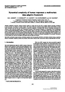
FIG. 2. (Color online) Dependence of the dynamical complexity at the node level and its topological role in a SF network of N = 150 R¨ ossler oscillators. (a) Complexity values Ci vs. d for different values of the node degree ki in a network with hki = 4. For the sake of comparison, the complete (E, black dashed line) and phase (R, black continuous line) synchronization curves are shown, rescaled for a better visualization. (b) hCik vs. k for the two coupling values d marked in (a) with vertical dashed lines, located before (d = 0.02) and after (d = 0.29) the phase synchronization transition. (c) hCik vs. the rescaled coupling dhki for the highest (filled markers) and lowest (void markers) node degree classes for three different mean degrees hki of the networks (see legend). Each point is the average of 10 network realizations.

full PS regime (vertical dashed line at d = 0.29 in panel (a)), the dependence is lost with hCik almost invariant with k. The negative correlation between hCik and k shown in Fig. S2(b) is not restricted to SF networks of neither identical nor phase coherent chaotic oscillators. In the Supplemental Material we report on the robustness of this relationship for a network of slightly different R¨ ossler oscillators by introducing some variability in the R¨ ossler natural frequencies. In addition, we also replaced the R¨ ossler oscillators by Lorenz chaotic ones, whose dynamics is far from being phase coherent, and obtained an equivalent hCik dependence on k for values of the coupling strength where the network is still not synchronous, as it can be seen in the Supplemental Information. To further explore the change in the dynamical complexity in the route to synchronization depending on the node degree, we varied the mean degree of the P (k). We found that the behavior scales with hki as shown in Fig. S2(c) for three different mean degrees, where the hCik is plotted vs. the rescaled coupling dhki. There, it is clear that the three curves of hCik for the nodes with the highest degree (filled markers) collapse up to exhibiting the same behavior with dhki, as well as those for the nodes with the lowest degree (void markers), whose decreasing trends are much less pronounced.

FIG. 3. (a) Phase order parameter R and synchronization error E vs. d for a star of N = 8 almost identical (within the 5% experimental tolerance) R¨ ossler-like electronic circuits (see the Supplementary Material for the system experimental description). (b) Dynamical complexity of the hub and of one of the leaves vs. d. Complexity measures are averaged over 30 different initial conditions and calculated over sequences of 5000 maxima with embedding length D = 3.

In order to provide some experimental evidence, we designed a star network with eight R¨ ossler-like chaotic electronic circuits. The reader is referred to Refs. [39–42] for a detailed description of the experimental implementation of the circuits and previous realizations in different network configurations. The results are presented in Fig. 3, where the synchronization state (Fig. 3(a)) and dynamical complexity C of the hub and of one of the leaves (Fig. 3(b)) are to be compared to their numerical counterparts in Fig. S1(a-b). Despite the natural parameter mismatch and environmental noise affecting our experimental set-up, the two markedly different paths of the dynamical complexities of both the hub and the leaves, a large loss in the hub and an almost constant level of complexity in the leaves, largely agree with those obtained in the numerical simulation, confirming the generality of the observation. The behavior can be understood analytically by performing a mean field approximation and a linear stability analysis of the actual state of each oscillator in the weakly coupling regime where the system is still far from reaching the same collective state [25, 26]. The local mean field P ¯ i = ki−1 N that oscillator i is receiving is x j=1 aij h(xj ). In the case of a highly connected node (ki ≫ 1), its mean field can be well approximated by the global mean field PN ¯ i ∼ X, whose variance is, X = N −1 j=1 , h(xj ), that is x below the onset of synchronization, very small [25, 43]. Under this assumption, the contribution from the coupling term to the time evolution of the hubs in Eq. (1) is simply N X that can be neglected since it is either zero or a constant depending whether the attractor has a symmetry with respect to the origin. Therefore, the

4 governing equations for the hubs [25] are given by x˙i ≃ f (xi ) + dN X − dki h(xi )

(2)

that is, the hub’s dynamics is being modulated by a strong negative self-feedback term (−dki h(xi )) that stabilizes the unstable periodic orbits resulting in a more stable trajectory than the original uncoupled one [44]. To prove this, let us consider all the infinitesimal displacements δx from a given trajectory xi of a hub. The time evolution of the tangent vector δxi is given by the linearization of the Eq. (2): δ x˙ i = [Jf (xi ) − dki Jh(xi )] δxi

(3)

where J stands for the Jacobian matrix. The solution to the variational equations of the perturbations results in an exponentially growth at a rate given by the Lyapunov exponents, whose maximum is given by Λ(k) = Λ0 − dki where Λ0 is the maximum positive Lyapunov exponent corresponding to a chaotic uncoupled oscillator and, without loss of generality, assuming that the coupling function h is linear. As a consequence, the trajectory will become dynamically less complex as a linear function of k, as observed in Fig. S2(b). Eventually, if the original node is chaotic and highly connected, it can become periodic with the consequent loss of statistical complexity. On the contrary, for the less connected nodes ki ∼ 1, in the weakly coupling regime, the diffusive term is too small as to modify the trajectory, and the node dynamics retains most of its original complexity. So far we have considered the node dynamics to be continuous and deterministic, which is a strong limitation in the potential application to real systems where noise is unavoidable. Therefore, we investigated whether the existing relationship between structure and chaotic flows at the micro-scale still holds in a network of pulse coupled neurons. We implemented the bio-inspired Morris-Lecar (ML) model [4] for type II excitatory neurons (with a discontinuous frequency-current response curve), whose equations describing the membrane potential behavior for each unit read [46]: C V˙i = −gCa M∞ (Vi − VCa ) − gK Wi (Vi − Vk ) −gl (Vi − Vl ) + qξi + Ii , W˙ i =φ τW (W∞ − Wi )

10-3 (a)

6

(4)

where Vi and Wi are, respectively, the membrane potential and fraction of open K + channels of the ith neuron and M∞ , W∞ , and τW are hyperbolic functions dependent on Vi and φ is a reference frequency. The parameters gX and VX account for the electric conductance and equilibrium potentials of the X = {K, Ca, leaky} channel. Parameter values are chosen such that neurons are subthreshold to neuronal firing which is induced by the white Gaussian noise qξi of zero mean and intensity q, and the d P −2(t−tj ) a (V0 − Vi ) injected synaptic current Ii = K j ij e

4

2 0 6

200 10

400

600

800

-3

(b) 5 4 3 5

10

15

20

25

30

35

40

FIG. 4. (Color online) Dependence of the dynamical complexity at the node level and its topological role in a SF network of N = 150 Morris-Lecar neurons. (a) Complexity values CT vs. d for low (k = 2) and high (k = 32) degree node values in a network with hki = 4. For the sake of comparison, the phase synchronization curve (R, black dotted line) is shown, rescaled for a better visualization. (b) CT vs. k for the two coupling values d marked in (a) with vertical dashed lines. Each point is the average of 10 network realizations.

given by the superposition of all the post-synaptic potentials emitted by the network in the past (see Supplemental Material for details). The typical neuronal dynamics exhibited by Eq. 4 when d = 0 consists of a sequence of spikes produced at random times tk whose amplitude variability is negligible. Therefore, we focused on the complexity Ci of the sequence of inter spike time tk − tk−1 patterns of each neuron. In order to quantify the level of synchronization among the network firing events we count how many neurons fire within the same time window. The total simulation time T is divided in n = 1, . . . , Nb bins of a convenient size τ , such that T = Nb τ , and the binary quantity Bi (n) is defined such that Bi (n) = 1 if the ith neuron spiked within nth interval and 0 otherwise. The coherence between the spiking sequence of neurons i and j is therefore characterized with the quantity sij ∈ [0, 1] PNb Bi (n)Bj (n) sij = PNb n=1 PNb , (5) B (n) n=1 i n=1 Bj (n)

where the term in the denominator is a normalization factor and sij = 1 means full coincidence between the two spiking series. The ensemble average of sij , S = PN hsij i = N (N2−1) i,j=1,i6=j sij is conveniently rescaled and reported in Fig. 4 as a dotted line indicating a transition from an asynchronous to an almost synchronous firing as the synaptic conductance d is increased. Superimposed to this curve are the complexities Ci of nodes with low (k = 2, blue dash-dotted line) and high (k = 32,

5 red solid line) degrees for 10 realizations of a SF network of N = 150 ML neurons. We observe that in this case of stochastic dynamics, as the coupling increases, the complexity of the highly connected nodes peaks at incipient levels of synchronization, as well as for the low degree nodes which occurs later. This is due to the fact that hubs are cross-talking with many nodes receiving low coherent noise-induced signals contributing to increase its own complexity. For larger values of the coupling strength (d = 300), still far from PS, the hubs complexity decreases as the information they are receiving is more coherent. In the bottom panel of Fig. 4, we show the correlation between the complexity hCik and the node degree at the two coupling strengths marked with dashed lines in the upper plot. Again, as in the case of the R¨ ossler network, a negative correlation of the complexity values with the number of synapses appears for intermediate values of the synchronization level. This suggests that, indeed, there is a region close to full synchronization where the complexity of a node can tell us about its degree. In this Letter, we have inspected the relationship between the topological role (degree) of a node in a complex network and its dynamical behavior (complexity). We showed both numerically and experimentally, that in a simple star of identical chaotic oscillators, the hub exhibits a minimum of complexity in the route to synchronization while the leaves almost keep unperturbed their

initial complex behavior. When considering more heterogeneous degree distributions (power-law kind), the same behavior is observed in the route to synchronization, with higher degree nodes exhibiting lower values of complexity. Importantly, when comparing the complexity of each node and its degree, we found a distinctive linear correlation with higher degree nodes exhibiting less complexity and that is generally observed in networks of other types of chaotic oscillators or pulse-coupled neurons. The reported results could explain recent observations about the low complexity of the hubs in functional brain networks [33] but, beyond than that, they suggest that the role played by the topology of a network could be unveiled by just computing the dynamical complexity associated with the time series sampled at each node. The fact that structural information of a network can be inferred without computing pairwise correlations like those commonly performed in functional networks could be exploited in diverse fields as neuroscience, econophysics or power grids. Financial support from the Ministerio de Econom´ıa y Competitividad of Spain (projects FIS2013-41057-P and FIS2017-84151-P) and from the Group of Research Excelence URJC-Banco de Santander is acknowledged. We thank J.M. Buld´ u for fruitful discussions. R.S.E. acknowledges support from Consejo Nacional de Ciencia y Tecnolog´ıa call SEP-CONACYT/CB-2016-01, grant number 285909.

[1] L. M. Pecora, Phys. Rev. E 58, 347 (1998). [2] M. Barahona and L. M. Pecora, Phys. Rev. Lett. 89, 054101 (2002). [3] S. Boccaletti, V. Latora, Y. Moreno, M. Chavez, and D.U. Hwang, Phys. Rep. 424, 175 (2006). [4] A. Arenas, A. D´ıaz-Guilera, J. Kurths, Y. Moreno, and C. Zhou, Phys. Rep. 469, 93 (2008). [5] E. Bullmore and O. Sporns, Nat. Rev. Neurosci. 10, 186 (2009). [6] M. Rohden, A. Sorge, M. Timme, and D. Witthaut, Phys. Rev. Lett. 109, 064101 (2012). [7] A. Pluchino, V. Latora, and A. Rapisarda, Int. J. Mod. Phys. C 16, 515 (2005). [8] N. Fujiwara, J. Kurths, and A. D´ıaz-Guilera, Phys. Rev. E 83, 025101 (2011). [9] E. Rodriguez, N. George, J. P. Lachaux, J. Martinerie, B. Renault, and F. J. Varela, Nature 397, 430 (1999). [10] L. Jean-Philippe, R. Eugenio, M. Jacques, and V. F. J., Human Brain Mapping 8, 194 (1999). [11] L. M. Pecora, F. Sorrentino, A. M. Hagerstrom, T. E. Murphy, and R. Roy, Nature Communications 5, 4079 (2014). [12] G. Tononi, O. Sporns, and G. M. Edelman, Proc. Natl. Acad. Sci. 91, 5033 (1994). [2] A. A. Rad, I. Sendi˜ na Nadal, D. Papo, M. Zanin, J. M. Buld´ u, F. del Pozo, and S. Boccaletti, Phys. Rev. Lett. 108, 228701 (2012). [14] O. Sporns, Curr. Opinion Neurobiol. 23, 162 (2013). [15] A. Arenas, A. D´ıaz-Guilera, and C. J. P´erez-Vicente,

Phys. Rev. Lett. 96, 114102 (2006). [16] J. G´ omez-Garde˜ nes, Y. Moreno, and A. Arenas, Phys. Rev. Lett. 98, 034101 (2007). [17] D. Li, I. Leyva, J. A. Almendral, I. Sendi˜ na Nadal, J. M. Buld´ u, S. Havlin, and S. Boccaletti, Phys. Rev. Lett. 101, 168701 (2008). [18] C. J. Honey, O. Sporns, L. Cammoun, X. Gigandet, J. P. Thiran, R. Meuli, and P. Hagmann, Proceedings of the National Academy of Sciences 106, 2035 (2009). [19] A. Navas, J. A. Villacorta-Atienza, I. Leyva, J. A. Almendral, I. Sendi˜ na Nadal, and S. Boccaletti, Phys. Rev. E 92, 062820 (2015). [20] P. S. Skardal, D. Taylor, and J. Sun, Phys. Rev. Lett. 113, 144101 (2014). [21] M. P. Van Den Heuvel and O. Sporns, Trends Cogn. Sci. 17, 683 (2013). [22] D. Papo, M. Zanin, J. A. Pineda-Pardo, S. Boccaletti, J. M. Buldu, and J. M. Buld´ u, Phil. Trans. R. Soc. B 369, 20130525 (2014). [23] G. Zamora-L´ opez, Y. Chen, G. Deco, M. L. Kringelbach, and C. Zhou, Sci. Rep. 6, 38424 (2016). [24] G. Deco, T. J. Van Hartevelt, H. M. Fernandes, A. Stevner, and M. L. Kringelbach, NeuroImage 146, 197 (2017). [25] T. Pereira, Phys. Rev. E 82, 036201 (2010). [26] C. Zhou and J. Kurths, Chaos 16, 015104 (2006). [27] R. L´ opez-Ruiz, H. Mancini, and X. Calbet, Phys. Lett. A 209, 321 (1995). [28] M. Martin, A. Plastino, and O. Rosso,

1 Phys. Lett. A 311, 126 (2003). [29] P. Lamberti, M. Martin, A. Plastino, and O. Rosso, Physica A 334, 119 (2004). [1] C. Bandt and B. Pompe, Phys. Rev. Lett. 88, 174102 (2002). [31] J. M. Amig´ o, K. Keller, and V. A. Unakafova, Phil. Trans. R. Soc. A 373, 20140091 (2018). [32] A. Politi, Phys. Rev. Lett. 118, 144101 (2017). [33] J. H. Mart´ınez, M. E. L´ opez, P. Ariza, M. Chavez, J. Pineda-Pardo, D. L´ opez-Sanz, P. Gil, F. Maest´ u, and J. M. Buld´ u, Sci. Rep. 8, 10525 (2018). [34] M. Barreiro, A. C. Marti, and C. Masoller, Chaos 21, 013101 (2011). [35] A. Schnurr, Stat. Papers 55, 919 (2014). [36] M. Zanin, L. Zunino, O. A. Rosso, and D. Papo, Entropy 14, 1553 (2012). [5] O. E. R¨ ossler, Phys. Lett. A 57, 397 (1976). [38] R. Albert and A.-L. Barab´ asi, Rev. Mod. Phys. 74, 47 (2002).

[39] R. Sevilla-Escoboza, R. Guti´errez, G. Huerta-Cuellar, S. Boccaletti, J. G´ omez-Garde˜ nes, A. Arenas, and J. M. Buld´ u, Phys. Rev. E 92, 032804 (2015). [40] R. Sevilla-Escoboza, I. Sendi˜ na Nadal, I. Leyva, R. Guti´errez, J. M. Buld´ u, and S. Boccaletti, Chaos 26, 065304 (2016). [41] I. Leyva, R. Sevilla-Escoboza, I. Sendi˜ na Nadal, R. Guti´errez, J. Buld´ u, and S. Boccaletti, Sci. Rep. 7, 45475 (2017). [42] I. Leyva, I. Sendi˜ na-Nadal, R. Sevilla-Escoboza, V. P. Vera-Avila, P. Chholak, and S. Boccaletti, Sci. Rep. 8, 8629 (2018). [43] M. G. Rosenblum and A. S. Pikovsky, Phys. Rev. Lett. 92, 114102 (2004). [44] S. Boccaletti, C. Grebogi, Y.-C. Lai, H. Mancini, and D. Maza, Phys. Rep. 329, 103 (2000). [4] C. Morris and H. Lecar, Biophys. J. 35, 193 (1981). [46] B. Sancrist´ obal, R. Vicente, J. M. Sancho, and J. Garc´ıaOjalvo, Front. Comput. Neurosci. 7, 18 (2013).

Supplementary Material: Dynamical complexity as a proxy for the network degree distribution I.

ORDINAL PATTERNS

We make use of the ordinal patterns [S1] formalism. This formalism associates a symbolic sequence to a time series, transforming the actual values of the measure into a set of natural numbers. Specifically, it works as follows: firstly, we have to decide what is going to be the size (D) of the bins that we are going to chop the time series in; then, for a given bin, we compare the values of the time series and order them in terms of its relative amplitudes. [S2] The main reasons to have chosen this method are the following: it is a classical, broad-field, well-established and known method, statistically reliable and robust to noise, extremely fast in computation and with a clear definition and interpretation in physical terms. It is derived from two also well-established measures (divergence and entropy), also easily interpretable when analyzing non linear dynamical systems. In addition, it only requires a soft criteria, namely that the time series must be pseudo-stationary and that M >> D! (where M is the number of points of the entire time series), which are easily checkable. Once we have the semantic signal, i.e. the natural numbers according to the ordinal patterns formalism, we proceed in the following way: 1. We count how many times each pattern appears (Nπ ). 2. We then define a probability of occurrence for each pattern: Pπ = in which we divide the time series, i.e. NT = N/D.

Nπ NT

, where NT is the total number of patterns

3. We construct an empirical probability distribution, which we call P from now on, from the pool of Pπ . We end up with a probability distribution P , constructed from the time series. We can now define the dynamical complexity measure we have used.

II.

ON THE WAY TO THE COMPLEXITY MEASURE

They key problem when trying to assign a value of the complexity of a time series is that the very definition of this quantity is a blurred line. Here we adopt the view that the Complexity should not arbitrarily grow but take into account the regime between pure noise and absolute regularity. Being this so, we need to characterize the disorder and a correcting term (i.e., a way of comparing known probability distributions with the actual one). In the main text, we took the path of defining the dynamical complexity (C) as the product of other two quantities: the Permutation Entropy (H) and the Disequilibrium (Q).

2 As it not evident how to get to that stage, we will begin by defining the classic Shannon entropy, that gives an idea of the disorder of the system: S[P ] = −

D! X

pj · log(pj )

(S1)

j=1

A simple normalization (specifically, the value of the entropy of the uniform probability distribution), Smax already yields the definition of our first ingredient, the Permutation Entropy: H=

S , Smax

Smax = S[Pe ],

Pe ≡ {1/D!}1,...,D! =⇒ 0 ≤ H ≤ 1

(S2)

Regarding the Disequilibrium, we have to introduce a way of comparing our actual probability distribution with the uniform one. A notion of distance can be acquired by several means; in this text, we adopt the statistical distance given by the Kullback-Leibler [S3] relative entropy (K): K[P |Pe ] = −

D! X

pj · log(pe ) +

D! X

pj · log(pj ) = S[P |Pe ] − S[P ]

(S3)

j=1

j=1

where S[P |Pe ] is the Shannon cross entropy. If we now symmetrize (S3), we get the Jensen-Shannon divergence (J): J[P |Pe ] = (K[P |Pe ] + K[Pe |P ])/2

(S4)

For our purposes, it is highly convenient to write (S4) in terms of S solely: J[P |Pe ] = S[(P + Pe )/2] − S[P ]/2 − S[Pe ]/2

(S5)

Finally, we can write the Disequilibrium (Q) as the normalized version of J as: Q = Q0 J[P |Pe ]

(S6)

−1

with Q0 = NN+1 log(N + 1) − 2 log(2N ) + log(N ) , implying again 0 ≤ Q ≤ 1. Having the exact mathematical form of both of its constituents, one can then define the Complexity (C) as: C = H · Q, III.

0≤C≤1

(S7)

THE MORRIS-LECAR MODEL

In the main text, we briefly mentioned the results of working with this bio-inspired model [S4]. Let us expand what are their constituents. The two main equations are given by: C V˙i = −gCa M∞ (Vi ) · (Vi − VCa ) − gK Wi (Vi − Vk )− gl (Vi − Vl ) + qξi + Isyn,i ,   ˙ Wi =φτw (Vi ) W∞ (Vi ) − Wi

(S8)

where Vi is the membrane potential, Wi is the recovery variable for the K channel, gCa , gK and gl are respectively the conductance of the Ca,K and leaky channels, VCa , VK and Vl are the resting electric potentials of the channels, and ξi is local white Gaussian noise of amplitude q. There are other ingredients in this model: the auxiliary functions. These are:       1h Vi − V1 i Vi − V3 i 1h Vi − V3 M∞ (Vi ) = 1 + tanh , W∞ (Vi ) = 1 + tanh , τw (Vi ) = cosh (S9) 2 V2 2 V4 2V4 for the sake of concreteness and replicability, we introduce table I, in which we detail the values of the parameters we used in the simulations. The highlight has been placed in the value of V3 because it is the parameter that lets us change the excitability type of the neuron. In this work, we have chosen V3 = 2.0 mV, which corresponds to a type II excitability neuron class (meaning a discontinous transition in the I − f domain). If we had used V3 = 12.0 mV instead, we would have been working with a type I excitability neuron.

3 C gCa gK gl VCa VK Vl V1 V2 V3 V4 φ

20.0 µF/cm2 4.0 µS/cm2 8.0 µS/cm2 2.0 µS/cm2 120.0 mV −80.0 mV −60.0 mV −1.2 mV 18.0 mV 2.0 mV 17.4 mV 1/15

TABLE I. Parameters used for the Morris-Lecar simulations.

IV.

¨ THE ROSSLER OSCILLATOR REVISITED

As we have already delved into a lot of detail in the main text to explain how this model [S5] behaves, we will directly move on to explain the next step we took to check the robustness of our results. In the case presented in the main text, we assumed that each oscillator had the very same parameters. We now let the internal frequency of each node to be slightly different, according to the homogeneous distribution Ωi = Ω0 ± δΩ; in this case, Ω0 = 1 and |δΩ| = 0.05, meaning that Ωi ∈ [0.95, 1.05]. The results of a N = 150 Scale-Free network, hki = 4, with this frequency dispersion, are portrayed in S1 (a)

(b)

CA

0.2 0.1 0 0

0.05

d

0.1

5

10

15

20

k

FIG. S1. Dynamical complexity C anti-correlates with the degree. All the measures are averaged over 10 initial conditions, storing sequences of maxima of length 104 per node, using D = 4 as the embedding length for the permutation patterns.

We again recover the correlation between the dynamical complexity and the degree of a certain node. The final test we have tried is to repeat this process with another model: the Lorenz oscillator.

4 V.

THE LORENZ OSCILLATOR

In order to check the robustness of our results, we wanted to add an extra model, which was different from the previous ones we used. The Lorenz oscillator [S6] was chosen because, although it is a chaotic oscillator like the R¨ ossler model, its attractor is quite different from the latter one. P Specifically, we used the network version of this oscillator, which consists in x˙ i = f (xi ) − d j Lij h(xj ), where
f (xi ) = 10 · (y − x), x · (28 − z) − y, xy − (8/3)z is the function governing the node dynamics, x ≡ (x, y, z) as the state vector, h(x) = (0, y, 0) is the output function and d is the coupling strength. L = {Lij } is the Laplacian matrix describing the coupling structure, with Lij = ki δij − aij where ki is the node degree, and A = {aij } the adjacency matrix, being aij = 1 if there is a link between nodes i, j and aij = 0 otherwise. To enable us to compare with the rest of our results, we simulated the same complex network as in the other cases: a Scale-Free made of 150 nodes, with hki = 4. The results are summed up in [fig S2]. (a)

(b)

CA

0.2 0.1 0 0

0.1

0.2

d

5

10

15

20

k

FIG. S2. (Color online) (a) Different curves for complexities against the coupling strength (see the main text for the parameter values). Each line represents (b) Dynamical complexity C anti-correlates with the degree. All the measures are averaged over 10 initial conditions, storing sequences of maxima of length 104 per node, using D = 4 as the embedding length for the permutation patterns.

We see that the main result is reproduced here: there is a correlation between the dynamical complexity C and the degree. In other words: it is possible to rank the topological relevance of a node only based in individual dynamical measurements.

[S1] C. Bandt and B. Pompe, Phys. Rev. Lett. 88, 174102 (2002). [S2] A. A. Rad, I. Sendi˜ na Nadal, D. Papo, M. Zanin, J. M. Buld´ u, F. del Pozo, and S. Boccaletti, Phys. Rev. Lett. 108, 228701 (2012). [S3] S. Kullback and R. A. Leibler, “On Information and Sufficiency,” . [S4] C. Morris and H. Lecar, Biophys. J. 35, 193 (1981). [S5] O. E. R¨ ossler, Phys. Lett. A 57, 397 (1976). [S6] E. N. Lorenz, Journal of the Atmospheric Sciences (1963), 10.1175/1520-0469(1963)020¡0130:DNF¿2.0.CO;2, arXiv:NIHMS150003.