Dynamical fidelity of a solid-state quantum computation

Dynamical fidelity of a solid-state quantum computation G.P. Berman[a] , F. Borgonovi[b,c], G. Celardo[b,d], F.M. Izrailev[e] , and D.I.Kamenev[a] [a]

arXiv:quant-ph/0206158v1 21 Jun 2002

Theoretical Division and CNLS, Los Alamos National Laboratory, Los Alamos, New Mexico 87545 [b] Dipartimento di Matematica e Fisica, Universit` a Cattolica, via Musei 41, 25121 Brescia, Italy [c] I.N.F.M., Unit´ a di Brescia and I.N.F.N., Sezione di Pavia, Italy [d] I.N.F.M., Unit` a di Milano, Italy [e] Instituto de F´isica, Universidad Aut´ onoma de Puebla, Apdo. Postal J-48, Puebla 72570, Mexico In this paper we analyze the dynamics in a spin-model of quantum computer. Main attention is paid to the dynamical fidelity (associated with dynamical errors) of an algorithm that allows to create an entangled state for remote qubits. We show that in the regime of selective resonant excitations of qubits there is no any danger of quantum chaos. Moreover, in this regime a modified perturbation theory gives an adequate description of the dynamics of the system. Our approach allows to explicitly describe all peculiarities of the evolution of the system under time-dependent pulses corresponding to a quantum protocol. Specifically, we analyze, both analytically and numerically, how the fidelity decreases in dependence on the model parameters. PACS numbers: 05.45Pq, 05.45Mt, 03.67Lx

I.

INTRODUCTION

Many suggestions for an experimental realization of quantum computers are related to two-level systems (qubits). One of the serious problems in this field is a destructive influence of different kinds of errors that may be dangerous for the stability of quantum computation protocols. In the first line, one should refer to finite temperature effects and interaction of qubits with an environment [1]. However, even in the case when these features can be neglected, errors can be generated by the dynamics itself. This “dynamical noise” can not be avoided since the interaction between qubits and with external fields are both necessary for the implementation of any quantum protocol. On the other hand, the inter–qubit interaction may cause the errors. Therefore, it is important to know to what extent the interaction effects may be dangerous for quantum computation. As is known from the theory of interacting particles, a two-body interaction between particles may result in the onset of chaos and thermalisation, even if the system under consideration consists of a relatively small number of particles (see, for example, the reviews [2, 3, 4] and references therein). In application to quantum computers, quantum chaos may play a destructive role since it increases the system sensitivity to external perturbations. Simple estimates obtained for systems of L interacting spins show that with an increase of L the chaos border decreases, and even a small interaction between spins may result in chaotic properties of eigenstates and spectrum statistics. On this ground, it was claimed [5] that quantum chaos for a large number of qubits can not be avoided, and the idea of a quantum computation

meets serious problems. On the other hand, recent studies [6] of a realistic 1/2spin model of a quantum computer show that, in the presence of a magnetic field gradient, the chaos border is independent on L, and that quantum chaos arises in extreme situations only, which are not interesting from the practical viewpoint. One should stress that a non-zero gradient magnetic field is necessary in the model [6] for a selective excitation of different qubits under time-dependent electromagnetic pulses providing a specific quantum protocol. Another point that should be mentioned in the context of quantum chaos is that typical statements about chaos refer to stationary eigenstates and spectrum statistics. However, quantum computation is essentially a time-dependent problem. Moreover, the time of computation is restricted by the length of a quantum protocol. Therefore, even if stationary Hamiltonians for single pulses reveal chaotic properties, it is still not clear to what extent stationary chaos influences the evolution of a system subjected to a finite number of pulses. In contrast with our previous studies [6], in this paper we investigate a time evolution of a 1/2-spin quantum computer system subjected to a series of pulses. Specifically, we consider a quantum protocol that allows to create an entangled state for remote qubits. For this, we explore the model in the so-called selective regime, using both analytical and numerical approaches. Our analytical treatment shows that in this regime there is no any fingerprint of quantum chaos. Moreover, we show that a kind of perturbation approach provides a complete description of the evolution of our system. We concentrate our efforts on the introduced quantity

2 (dynamical fidelity). This quantity characterizes the performance of quantum computation associated with the dynamical errors. Dynamical fidelity differs from the fidelity which is associated with the external errors, and which is widely used nowadays in different applications to quantum computation and quantum chaos, see for instance [7]. Our study demonstrates an excellent agreement of analytical predictions with numerical data. The structure of the paper is as follows. In Section II we discuss our model and specify the region of parameters for which our study is performed. In Section III we explore a possibility of quantum chaos in the selective regime, and analytically show that chaos can not occur in this case. We provide all details concerning the quantum protocol in Section IV, and demonstrate how perturbation theory can be applied to obtain an adequate description of the fidelity in dependence on the system parameters. Here, we also present numerical data and compare them with the predictions based on the perturbative approach. The last Section V summarizes our results.

In our model the spin chain is also subjected to a transversal circular polarized magnetic field. Thus, the expression for the total magnetic field has the form [6, 10, 11], ~ B(t) = [bp⊥ cos(νp t + ϕp ), −bp⊥ sin(νp t + ϕp ), B z (x)]. (1) As is mentioned above, here B z (x) is the constant magnetic field oriented in the positive x-direction, with a positive x-gradient (therefore, a > 0 in the expression for the Larmor frequencies). In the above expression, bp⊥ , νp , and ϕp are the amplitudes, frequencies and phases of a circular polarized magnetic field, respectively. The latter is given by the sum of p = 1, ..., P rectangular time-dependent pulses of length tp+1 − tp , rotating in the (x, y)− plane and providing a quantum computer protocol. Thus, the quantum Hamiltonian of our system has the form,   L−1 P P z z z Jk,n Ik In − ωk Ik + 2 H=− n>k

k=0

II.

SPIN MODEL OF A QUANTUM COMPUTER

Our model is represented by a one-dimensional chain of L identical 1/2-spins placed in an external magnetic field. It was first proposed in [8] (see also [9, 10, 11]) as a simple model for solid-state quantum computation. Some physical constraints are necessary in order to let it operate in a quantum computer regime. To provide a selective resonant excitation of spins, we assume that the time independent part B z = B z (x) of a magnetic field is non-uniform along the spin chain. The non-zero gradient of the magnetic field provides different Larmor frequencies for different spins. The angle θ between the direction of the√chain and the z-axis satisfies the condition, cos θ = 1/ 3. In this case the dipole-dipole interaction is suppressed, and the main interaction between nuclear spins is due to the Ising-like interaction mediated by the chemical bonds, as in a liquid state NMR quantum computation [1]. In order to realize quantum gates and implement operations, it is necessary to apply selective pulses to single spins. The latter can be distinguished, for instance, by imposing constant gradient magnetic field that results in the Larmor frequencies ωk = γn B z (xk ) = ω0 + ak, where γn is the spin gyromagnetic ratio and ak = xk and xk is the position of the k-th spin. If the distance between the neighboring nuclear spins is ∆x = 0.2 nm, and the frequency difference between them is ∆f = a/2π = 1 kHz, then the corresponding gradient of the magnetic field can be estimated as follows, |dB z /dx| = ∆f /(γn /2π)∆x ≈ 1.2 × 104 T/m. Here we used the gyromagnetic ratio for a proton, γn /2π ≈ 4.3 × 107 Hz/T. Such a magnetic field gradient is experimentally achievable, see, for example, [12, 13].

1 2

P P

Θp (t)Ωp

p=1

L−1 P k=0

!

(2)

e−iνp t−iϕp Ik− + eiνp t+iϕp Ik+ ,

where the “pulse function” Θp (t) equals 1 only during the p-th pulse, for tp < t ≤ tp+1 , otherwise, it is zero. The quantities Jk,n stand for the Ising interaction between two qubits , ωk are the frequencies of spin precession in the B z −magnetic field, Ωp is the Rabi frequency of the p-th pulse, Ikx,y,z = (1/2)σkx,y,z with σkx,y,z as the Pauli matrices, and Ik± = Ikx ± iIky . For a specific p-th pulse, it is convenient to represent the Hamiltonian (2) in the coordinate system that rotates with the frequency νp . Therefore, for the time tp < t ≤ tp+1 of the p-th pulse our model can be reduced to the stationary Hamiltonian, H(p) = −

L−1 P k=0

(ξk Ikz + αIkx − βIky ) − 2

P

n>k

Jk,n Ikz Inz ,

(3) where ξk = (ωk − νp ), α = Ωp cos ϕp , and β = Ωp sin ϕp . We start our considerations with the simplified case of the Hamiltonian (3) for a single pulse, by choosing ϕp = 0. We also assume a constant interaction between nearest qubits only (Jk,n = Jδk,k+1 ), and we put Ωp = Ω. Then the Hamiltonian (3) takes the form, H

(p)

=

L−1 Xh k=0

z −ξk Ikz −2JIkz Ik+1

i

−Ω

L−1 X k=0

Ikx ≡ H0 +V. (4)

In the z-representation the Hamiltonian matrix of size 2L is diagonal for Ω = 0. For Ω 6= 0, non-zero off-diagonal matrix elements are simply Hkn = Hnk = −Ω/2 with n 6= k. The matrix is very sparse, and it has a specific structure in the basis reordered according to an increase

3 of the number s. The latter is written in the binary representation, s = iL−1 , iL−2 , ..., i0 (with is = 0 or 1, depending on whether the single-particle state of the i−th qubit is the ground state or the excited one). The parameter Ω thus is responsible for a non-diagonal coupling, and we hereafter define it as a “perturbation”. In our previous studies [6] we have analyzed the socalled non-selective regime which is defined by the conditions, Ωp ≫ δωk ≫ J. This inequality provides the simplest way to prepare a homogeneous superposition of 2L states needed for the implementation of both Shor and Grover algorithms. Our analytical and numerical treatment of the model (2) in this regime has shown that a constant gradient magnetic field (with non-zero value of a) strongly reduces the effects of quantum chaos. Namely, the chaos border turns out to be independent on the number L of qubits. As a result, for non-selective excitation quantum chaos can be practically neglected (see details in [6]). Below we consider another important regime called selective excitation. In this regime each pulse acts selectively on a chosen qubit, resulting in a resonant transition. During the quantum protocol, many such resonant transitions take place for different p pulses, with different values of νp = ωk . The region of parameters for the selective excitation is specified by the following conditions [10], Ωp ≪ Jk,n ≪ a ≪ ωk .

|...0, 1, 0...i |...1, 1, 1...i |...1, 1, 0...i |...0, 1, 1...i

(5)

The meaning of these conditions will be discussed in next Sections. III.

speaking, the above condition in a strong sense (Ω ≫ δf ) means that exact eigenstates consist of many unperturbed (V = 0) states. Typically, the components of such compound states can be treated as uncorrelated entries, thus resulting in a chaotic structure of excited manybody states. However, one should note that in specific cases when the total Hamiltonian is integrable (or quasiintegrable), the components of excited states have strong correlations and can not be considered as chaotic, although the number of components with large amplitudes can be extremely large (see details in [6]). It is relatively easy to estimate Mf in the regime of selective excitation. Let us consider an eigenstate of H0 , |1, 0, 0, 0, 1, 0, ..., 0, 0, 1, 0i, as a collection of 0’s and 1’s that correspond to −1/2 and 1/2-spin values. Since the perturbation V is a sum of L terms, each of them flipping one single spin, one gets Mf ∼ L. In order to estimate (∆E)f , let us first consider the action of V on the k-th spin, and for each spin compute the relative energy difference between the final and the initial energy. One can find that if the k-th spin has the value 1/2, there are four possible configurations of neighbor spins coupled by the perturbation,

Ω (∆E)f . > δf ≈ 2 Mf

(6)

Here (∆E)f is the maximal difference between the ener(2) (1) gies E0 and E0 corresponding to a specific many-body state |1i , and all other states |2i of H0 , that have nonzero couplings h1|V |2i. Correspondingly, Mf is the number of many-body states |2i coupled by V to the state |1i. A further average over all states |1i should be then performed. In fact, such a comparison (6) is just the perturbation theory in the case of two-body interaction. Strictly

(7)

If the k-th spin has the value −1/2, there are also four possible different arrangements, |...0, 0, 0...i |...1, 0, 1...i |...1, 0, 0...i |...0, 0, 1...i

ABSENCE OF QUANTUM CHAOS IN THE SELECTIVE EXCITATION REGIME

Here, we consider the properties of the stationary Hamiltonian (4) in the regime of selective excitation. In order to estimate the critical value of the interaction J, above which one can expect chaotic properties of eigenstates, one needs to compare the typical value of the offdiagonal matrix elements (which is Ω/2) with the mean energy spacing δf for unperturbed many-body states that are directly coupled by these matrix elements. Therefore, the condition for the onset of chaos has the form,

→ |...0, 0, 0...i, → |...1, 0, 1...i, → |...1, 0, 0...i, → |...0, 0, 1...i.

→ |...0, 1, 0...i, → |...1, 1, 1...i, → |...1, 1, 0...i, → |...0, 1, 1...i,

(8)

which are the inverse transitions of (7). Correspondingly, the energy changes are determined by the relation, (f )

|E0

(i)

− E0 | = |ξk ± 2J|, |ξk |,

k = 1, ..., L − 2. (9)

The analysis for the border spins can be performed in a similar way, and one gets four possible configurations, with the following energy changes, (f )

|E0

(i)

− E0 | = |ξk ± J|,

k = 0, L − 1.

(10)

Summarizing the above findings, and setting for instance νp = ω0 , one can conclude that (∆E)f can be estimated as follows, (f )

(∆E)f = M ax(|E0

(i)

− E0 |) = ωL−1 − ω0 + J.

(11)

As a result, the condition for the onset of quantum chaos can be written in the form, ωL−1 − ω0 + J (∆E)f a(L − 1) + J Ω = > = , 2 Mf L L

(12)

4 or Ω > Ωcr ≃ a +

J . L

(13)

However, this critical value is outside the range of parameters required to be in the selective excitation regime Ω < a (see inequality (6)). Thus, we can conclude that quantum chaos for stationary states can not appear in the selective excitation regime. Note that the analysis is done for a single pulse of a time-dependent perturbation. IV.

FIDELITY OF A QUANTUM PROTOCOL

Analytical results obtained above, show that during a single electromagnetic pulse the system can be described by perturbation theory. Indeed, if matrix elements of perturbation are smaller than the energy spacing between directly coupled many-body states, exact eigenstates can be obtained by perturbation theory. Thus, one can expect that for a series of time-depended pulses the evolution of the systems can be also treated making use of a kind of perturbative approach. In what follows, we study the dynamics of the system by applying a specific set of pulses (quantum protocol) in order to create an entangled state for remote qubits (with k = 0 and k = L − 1) starting from the ground state, |ψ0 i = |0L−1 , ..., 01 , 00 i (we omit the subscripts below). Our main interest is in estimating the errors that appear due to unwanted excitations of qubits. We show that these errors can be well understood and estimated on the basis of the perturbation theory developed for our time-dependent Hamiltonian (2), in the parameter range where the protocol holds. A.

Selective excitation regime and perturbation theory

Any protocol is a sequence of unitary transformations applied to some initial state in order to obtain a final state, |ψ i i. In this model of quantum computer the protocol is realized by applying a number of specific rfpulses, so that we get a state |ψ r i which is, in principle, different from the ideal state |ψ i i. The difference between the final state |ψ r i and the ideal state |ψ i i can be characterized by a dynamical fidelity, F = |hψ i |ψ r i|2 .

(14)

Note that, in our case the dynamical fidelity F does not explicitly depend on a perturbation parameter added in the Hamiltonian (2) in order to get a distorted evolution, as is typically assumed in the study of quantum chaos. Indeed, the final state is determined by the total Hamiltonian (2), R tp P Y −i H(t)dt tp−1 ˆ (T )|ψ0 i ≡ Tˆe |ψ0 i, (15) |ψ r i = U p=1

ˆ (T ) where T = tp is the total time to entangle spins, U is the unitary operator given by the sequence of pulses in the protocol, and Tˆ− is the usual time-ordered product. Therefore, it is not possible to identify a single perturbation parameter which is responsible for a “wrong” evolution of the system. The selective excitation regime is characterized by the action of pulses that are resonant with a transition between two energy states which differ for the state (up or down) of one spin only. A close inspection of the time independent Hamiltonian (4), defines the region of parameters where the selective excitation of single spins can be performed. Diagonal elements of Hamiltonian (4) are given by the (i) eigenvalues E0 of H0 , while non-zero off-diagonal elements are constant and equal to −Ω/2. In order to have a resonant transition between two energy states, their energy difference ∆ has to be zero. On the other side, for each state no more than one resonant transition should be allowed. So, we require that the energy differences given by Eqs. (9,10) are different from zero (apart from the wanted transition). This leads to the following set of equalities (“fake transitions”), J J J J

= a k4 = a k2 = ak = a k3

when when when when

k = 1, ..., L − 3, k = 1, ..., L − 3, k = 1, ..., L − 2, k = 1, ..., L − 2,

(16)

From Eqs.(16) it is easy to see that first “fake” transition appears for J1 = a/4, the second for J2 = a/2 and so on up to the last one for Jf = a(L − 2). All these resonances can be avoided if we choose a ≫ 4J. Indeed, it is not enough to chose simply a > 4J since resonances have finite widths. Transitions can be defined according to their energy difference ∆, 1) resonant transitions, ∆ = 0; 2) near–resonant transitions, ∆ ∼ J; 3) non–resonant transitions, ∆ ∼ a. For a ≫ 4J, each state can undergo one resonant or near-resonant transition only, and many non-resonant ones. The latter can be neglected if we choose a ≫ Ω. Under these conditions we can form couples of states, connected by resonant or near-resonant transitions, and we can rearrange the Hamiltonian matrix (4) by 2 × 2 block matrices representing all resonant and near-resonant transitions. This allow us to describe the dynamical evolution of the system as a two-state problem. Using this procedure, the entire sequence of pulses can be evaluated. Note that special attention has to be paid to an additional phase shift that arises between any two pulses, due to the change of frame. We remind that the

5 transformation between the rotating and the laboratory frame is given by the expression, P z (17) |ψ(t)iLab = eiνp t k Ik |ψ(t)iRot

Indeed, let us consider an initial basis state |mi at time t = 0, and find the probability for a resonant (∆ = 0) or near-resonant (∆ ∼ J) transition to the state |pi with the energy difference Ep − Em . Here Ep and Em are the eigenenergies of the time-independent part of the Hamiltonian (2), written in the laboratory frame. Setting, X ψ(t) = cn (t)e−iEn t |ni, (18) n

and cp (0) = 0, the application of a pulse for a time τ gets: ∆ −i cm (τ ) = cm (0)[cos( λτ sin( λτ 2 ) + i λ ∆τ 2 )]e λτ Ω i 2 −iEp τ , cp (τ ) = cm (0)[i λ sin( 2 )]e

∆τ 2

−iEm τ

,

(19) √ where λ = Ω2 + ∆2 . Note that Eqs.(19) refer to the laboratory frame. As we can see, the parameter ǫ determined as ǫ=

τ p  Ω2 2 + ∆2 sin Ω Ω2 + ∆2 2

(20)

characterizes the probability of resonant and nearresonant transitions. In particular, the probability of unwanted near-resonant transitions goes like ǫ, and it can be reduced by assuming J ≫ Ω. Combining all the above expression, we get the condition (5). Correspondingly, the probability for a non-resonant transition (neglecting terms of the order 1/L, and assuming a ≫ Ω ) is given by the parameter η [11], η=

Ω2 . 4a2

(21)

We would like to stress that even if the ideal state has been constructed taking into account resonant transitions only, our dynamical fidelity is a measure of dynamical errors that are due to near and non-resonant transitions. Let us now briefly discuss the perturbative approach that is based on recent studies published in Ref.[11]. The main idea is that for each p-th pulse the unperturbed basis can be rearranged in such a way that the Hamiltonian matrix is represented by 2×2 block matrices, as described above. This is what we call unperturbed Hamiltonian for a specific p-th pulse. One should note that this unperturbed Hamiltonian is Ω-dependent. Let us now define by V the Ω-dependent part which is responsible for non-resonant transition and not described by the 2 × 2 block matrices. Then it is easy to obtain the unperturbed eigenstates, |ψq0 i, and the unperturbed eigenvalues, ǫ0q , by diagonalizing each of the 2 × 2 blocks independently.

After this step, one can compute the perturbed eigenstates by taking into account first order terms only, |ψq i = |ψq0 i +

X hψq0 |V|ψq0′ i |ψq0′ i. 0 − ǫ0 ǫ ′ q q ′

(22)

q 6=q

Note that this perturbative approach is supposed to be valid when Eqs.(16) are not satisfied, and when the errors due to near-resonant transitions are much larger than the errors due to non-resonant ones, ǫ ≫ η. B.

Quantum protocol

Let us briefly sketch the algorithm and the particular protocol which was developed in Ref. [10]. Starting from the ground state |ψ0 i = |0...0i and applying a number of specific pulses, we would like to generate the following entangled state, 1 |ψ i i = √ (|0...0i + |10....01i) . 2

(23)

This algorithm could serve, for instance, as the first step for a more general teleportation protocol, and for an implementation of conditional quantum logic operations. The algorithm can be realized in the following way (for details see Ref. [10]), |0, ..., 0i → (|0, ..., 0i + |1, 0, .., 0i) → (|0, ..., 0i + |1, 1, 0, .., 0i) → (|0, ..., 0i + |1, 1, 1, 0, .., 0i) → (|0, ..., 0i + |1, 0, 1, 0, .., 0i) → . . . → (|0, ..., 0i + |1, 0, .., 1i).

(24)

Physically, the above algorithm can be done by applying suitable rf-pulses that are resonant to the desired transitions. The latter are originated from induced Rabi oscillations between the resonant states. To flip the k-th spin we have to choose the frequency ν of the rf-pulse according to the relation νp = E1 − E2 , where |1i and |2i are the states involved in the transition and E1 and E2 are the eigenenergies of the timeindependent part of Hamiltonian (2). For instance, for the first pulse we have to set, ν1 = |E|1,0,...,0i − E|0,...,0i |, and we have to apply it for a time t1 = π/2Ω to get equal superposition of the states involved in the transition. For other pulses we require that the first state (|0, ..., 0i) remains the same (apart from an additional phase), while the second state flips the k−th spin. This amounts to say that the probability of unwanted states is due to non-resonant transitions of both states, and to near-resonant ones only of the first state in the r.h.s. of Eq.(24). Specifically, the state |0, ..., 0i undergoes nearresonant transitions with ∆ = 2J for each pulse, except the first one which is resonant, and the forth for which ∆ = 4J. One should also take into account that at each pulse the state |0, ..., 0i get an additional phase, see eqs.

6

where L ≫ 1. Before discussing our numerical results we would like to stress that in contrast to what is mainly considered in the literature, the time for our dynamical fidelity is not an independent variable. Indeed, the length of the protocol is determined by the total number of qubits, L. Specifically, 2L − 2 pulses are necessary in order to create the entangled state, so that the protocol time T is proportional to the number of qubits. C.

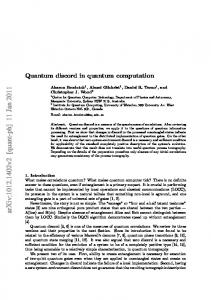
Dynamical fidelity: theory and numerical data

Quite unexpectedly, the dynamical fidelity (14) increases with an increase of the Ising coupling J, as soon as J ≪ a/4. This is due to the fact that the probability of unwanted near-resonant transitions is proportional to ǫ ∼ (Ω/J)2 (see Eq.(20) where ∆ ∼ J for near-resonant transitions ). The larger is J, the smaller is the probability of non-resonant transitions, therefore, the dynamical fidelity F increases with an increase of J. In Fig.1 we show how the dynamical fidelity (14) depends on the inter-qubit interaction J. For convenience, the function 1 − F is shown here and below, instead of F . Numerical data have been obtained in two different ways. Full curve corresponds to exact computation of the time-dependent Hamiltonian (2). Data in Fig.1a are compared with those obtained from the perturbative approach explained above. Apart from very strong peaks (see Fig.1b) for which the dynamical fidelity vanishes, one can say that the global tendency is an improvement of the dynamical fidelity for larger values of J. However, strong oscillations occur reflecting a resonant nature of the dynamics of our system. Perfect agreement between perturbative results and numerical data is found for very large variations of the interaction strength J. High peaks for 1 − F , clearly seen in Fig.1b, are due to Eqs.(16), in these points the quantum algorithm fails. Thus, one should avoid these situations in a quantum computation. As for the minima in Fig.1a for which the dynamical fidelity is close to one, they occur when ǫ = 0, or, when Ωp 2 J= 4k − 1, 2

0

10

Numerical Perturbative

−1

10

a)

1−F

−2

10

−3

10

−4

10

−5

10

0

0.5

1

1.5

2

J 1

b) 1−F

(19). We took them into account in the definition of the ideal state. Since in the selective excitation regime we have ǫ ≫ ν, contributions from near-resonant transitions are much larger than the one due to non-resonant transitions. Our algorithm consists of 2L − 2 separate pulses, therefore, some modifications are necessary in order to be able to control small unwanted probability. For the product of probabilities this requires to impose, 2Lǫ < 1 and 2Lη < 1, that can be written in the form, r r Ω Ω 2 2 ≪ , ≪ (25) J L a L

0.5

0

0

25

50

75

100

J FIG. 1: The dependence 1 − F is shown as a function of the Ising coupling J for L = 6 spins, Ω = 0.118 and a = 100. Full line represents the numerical data for the dynamical fidelity F defined by Eq.(14), and obtained from direct numerical computation of the system evolution. (a) Full circles stand for perturbative calculations, and full curve corresponds to numerical results. (b) The same numerical results as in (a), but for a larger range of J. The theoretical expression as given by Eq.(30) is also shown in (a).

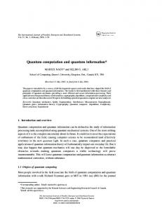
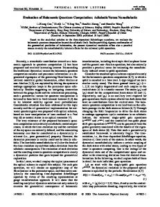
where k is an integer number. This relation corresponds to the 2πk-condition [10, 11, 14]. Let us now explore the dependence of the dynamical fidelity on the parameter a which is proportional to the gradient of the external magnetic field, a = γn ∆x(dB z (x)/dx), where ∆x is the distance between neighboring qubits. (Below, we shall refer to the parameter a as to the magnetic field gradient.) Numerical data for the dependence of 1 − F on a are presented in Fig.2. One can see that the dynamical fidelity is getting better for large enough values of a. We already mentioned that for a < 4J a problem may arise in the protocol due to “fake” transitions. On the other side, in the regime a ≫ 4J the dynamical fidelity reaches an asymptotic value which depends on J and Ω only, see Fig.2. It is also important to understand the dependence of the dynamical fidelity on the Rabi frequency Ω. The data manifest two specific properties demonstrated in Fig.3. The first one is a global decrease of the dynamical fidelity with an increase of Ω. The second peculiarity is due to strong oscillations that occur for ǫ = 0, namely for those Ω values that correspond to the 2πk-conditions, 2J . Ωk = √ 4k 2 − 1

(26)

For these values of Ω near-resonant transitions vanish, and non-resonant transitions remain only. Thus, the dynamical fidelity has maxima which provides, in principle,

7

1−F

10

0

10

−1

10

−2

is excellent. On the other hand, we cannot choose an extremely small value of Ω since it implies a large time duration of the pulse (τ ∼ π/Ω). Note, that the total time for a quantum protocol should be kept well below the decoherence time (the latter can be quite large for nuclear spins [15]). Taking this point into account, an optimal choice √ is to take the largest possible value, Ω = Ω2 = 2J/ 15 < J, and large enough value of a (in order to significantly suppress the non-resonant transitions). D.

10

−1

10

0

10

1

10

2

a FIG. 2: The dependence 1 − F as a function of the gradient of a magnetic field is shown for L = 6 spins, Ω = 0.118 and J = 1. As one can see, for a < 4J the correspondence is not so good as for a > 4J. 0

10

Numerical Perturbative

−1

10

Fidelity: dependence on the number of qubits

−2

10

Finally, we studied the dependence of the dynamical fidelity on the number L of spins in the chain. As was noted before, for a chosen protocol its length is proportional to L. Numerical data clearly manifest a linear decrease of the dynamical fidelity with the number of qubits, see Fig. 4. This dependence can be also understood on the basis of perturbation theory, by neglecting the change of phases between the ideal and the real state. This can be done since we already considered the main change of phases in the definition of the ideal state. Let us write, X |ψ r i = ck |ψk i, (27)

1−F

k

and assume that after M pulses the components c0 and c1 are, 1 1 √ (28) c1 = √ . c0 = √ 1 − M ǫ; 2 2

−3

10

−4

10

−5

10

k=8

k=7

k=6

−6

10

0.05

0.1

Ω

0.15

0.2

FIG. 3: The difference 1 − F as a function of the Rabi frequency Ω for L = 6 spins, J = 1 and a = 100. Full curve is the result of direct numerical simulation, circles are obtained from the perturbative approach described in the text. Arrows show few resonant values of Ω given by Eq.(26).

the best condition for a quantum computation. Nevertheless, let us consider the values of Ω that correspond to maxima in Fig.(3). This we do in order to make an estimate in the worst possible condition. A brief analysis of the fidelity for specific values Ω = Ωk will be sketched in the last subsection. As one can see, for values of Ω different from Ωk , the “average” dynamical fidelity increases when the Rabi frequency decreases. This is due to the fact that the probability to generate unwanted states (due to both non-resonant and nearresonant transitions), is proportional to (Ω/∆)2 . Therefore, the smaller is Ω the more reliable the algorithm is. Note that the agreement with the perturbative approach

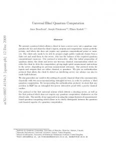
Here c0 and c1 are the complex amplitudes of two states in Eq.(23), but obtained as the result of the quantum protocol. This means that the probability of near-resonant states after M pulses is small, M ǫ ≪ 1. Then we get, √ 1 ǫ F = (2 − M ǫ + 2 1 − M ǫ) ∼ 1 − M , (29) 4 2 where ǫ ∼ Ω2 /4J 2 and M = 2L − 3 for our specific algorithm. Combining all the above expressions, one gets,   Ω2 3Ω2 F ∼ − 2L + 1 + , (30) 4J 8J 2 which implies a linear decrease of the dynamical fidelity with an increase of the number of qubits, L. The slope is given by the parameter mth = −Ω2 /4J 2 . Of course, this consideration is valid far from the resonant conditions (16). To compare numerical data with the above analytical estimate for mth , we obtained the slopes in Fig. 4 by the best fit to a linear dependence. These slopes versus J are shown in Fig. 5, together with the theoretical result for mth . As one can see, the agreement is very good except for small values of the Ising interaction, J ≃ Ω, where the probability of near-resonant transitions becomes large.

8 1

1.002

0,99998

1

0.998

F

F

0,99996

0.996 0,99994

J=5.01 0.994

J=9.99 0,99992

J= 1.945

0.992

0,9999

0.99

1

2

3

4

5

6

7

8

9

10

2

4

11

L FIG. 4: The dynamical fidelity as a function of the number L of spins, for different J values and Ω = 0.118, a = 100. Numerical data (triangles for J = 1.945, circles for J = 5.01 and squares for J = 9.99) are compared with the results from the perturbation theory (crosses). Also shown are the best linear fits (dot-dashed lines).

−m

10

0

10

−1

10

−2

10

−3

10

−4

10

−5

10

−6

10

Numerical mth

10

−1

10

0

10

1

10

2

J FIG. 5: Comparison between theoretical and numerical linear slopes for the fidelity, as a function of the interaction J.

E.

Optimal algorithm

Choosing Ω values as given by Eq.(26), one gets that the probability for near-resonant transition is zero, ǫ = 0. So, only non-resonant transitions lead to unwanted states. In Fig.(6) we show the fidelity as a function of the number of spins L for Ωk = 0.1216. These data should be compared with the analogous ones indicated by triangles in Fig.(4). As one can see, despite the closeness of these two Ω values (less than 3% of difference), the fidelity is better by two order of magnitude (see different scales on the y-

8

10

FIG. 6: The dynamical fidelity as a function of the number L of spins, for J = 1.945 and Ωk = 0.1216, a = 100. Also shown is the best linear fit with the slope 9.2 ± 0.3 × 10−6 .

axis). It is clear that such preferred Ω values should be chosen in any practical implementation of the algorithm. However, due to a high instability of such resonant values, see Fig.(3), the detailed analysis can only be done within a more general study under the presence of small variations in parameters such as Ω, J, a. This study is currently in progress. V.

−2

6

L

CONCLUSIONS

We have studied the model of a quantum computer that consists of a one-dimensional chain of 1/2-spins (qubits), placed in a time-dependent electromagnetic field. The latter is given by a sequence of rf-pulses, corresponding to a chosen quantum protocol that allows to generate an entangled state for remote qubits from the initial ground state. Main attention is paid to the analysis of the dynamical fidelity, defined as an overlap of the actual finite state, with the ideal one determined by the quantum protocol. We considered the region of the selective excitation where the resonant excitations of specific qubits can be implemented by time-dependent pulses. Analytical treatment of the stationary Hamiltonian which describes the evolution of the system during a single pulse, has revealed that in the selective regime the quantum chaos can not appear. Moreover, in this regime a perturbation theory can be applied to all quantities of interest. Our detailed study of the dynamical fidelity manifests excellent agreement between numerical data and the predictions obtained in the perturbative approach. In particular, we have found how to choose parameters of the model in order to get the best dynamical fidelity for the creation of the remote entangled state. Specific attention has been paid to the dependence of the dynamical fidelity on the number L of qubits. We show, both analytically

9 and numerically, that the dynamical fidelity decreases linearly with an increase of L, and we give an analytical estimate for the slope of this dependence. VI.

ACKNOWLEDGMENTS

The work of GPB was supported by the Department of Energy (DOE) under the contract W-7405-ENG-36,

[1] I.L. Chuang, R. Laflamme, P.W. Shor, and W.H. Zurek, Science, 270, 1633 (1995). [2] V. Zelevinsky, B.A. Brown, N. Frazier, and M. Horoi, Phys. Rep., 276, 85 (1996). [3] T. Guhr, A. M¨ uller-Groeling, and H.A. Weidenm¨ller, Phys. Rep., 299, 189 (1999). [4] V.K.B. Kota, Phys. Rep., 347, 223 (2001). [5] B. Georgeot and D.L. Shepelyansky, Phys. Rev. E., 62, 3504 (2000); ibid, 6366. [6] G.P. Berman, F. Borgonovi, F.M. Izrailev, and V.I. Tsifrinovich, Phys. Rev. E., 64 056226 (2001); Phys. Rev. E., 65, 015204 (2001). [7] A.Peres, Phys. Rev. A 30, 1610 (1984); R.A. Jalabert and H.M. Pastawski, Phys. Rev. Lett. 86, 2490 (2001); Ph. Jacquod, P.G. Silvestrov and C. W. J. Beenakker, Phys. Rev. E 64, 055203 (2001); N.R. Cerruti and S.Tomsovic, Phys. Rev. Lett. 88, 054103 (2002); T.Prosen, Phys. Rev. E 65, 036208 (2002); F.M. Cucchietti, C.H.Lewenkopf, E.R.Mucciolo, H.M. Pastawsky and R.O. Vallejos, Phys.

by the National Security Agency (NSA) and Advanced Research and Development Activity (ARDA). FMI acknowledges the support by CONACyT (Mexico) Grant No. 34668-E. We acknowledge R.Bonifacio for useful discussions. Authors also thanks the International Center at Cuernavaca for financial support during the workshop ”Chaos in few and many-body problems” where this work was started.

[8] [9] [10] [11] [12] [13] [14] [15]

Rev. E 65, 046209 (2002) ; G.Benenti and G.Casati, quant-ph/0112132; T.Prosen, T.H.Seligman, M.Znidaric, quant-ph/0204043. G.P. Berman, G.D. Doolen, G.D. Holm, V.I. Tsifrinovich, Phys. Lett. A , 193, (1994) 444. G.P. Berman, G.D. Doolen, R. Mainieri, and V.I. Tsifrinovich, Introduction to Quantum Computers, World Scientific Publishing Company, 1998. G.P. Berman, G.D. Doolen, G.V. L´ opez, and V.I. Tsifrinovich, Phys. Rev. A, 6106, 2305 (2000). G.P. Berman, G.D. Doolen, D.I. Kamenev, and V.I. Tsifrinovich, Phys. Rev. A, 6501, 2321 (2002). K.J. Bruland, W.M. Dougherty, J.L. Garbini, J.A. Sidles, S.H. Chao, Appl. Phys. Lett., 73, 3159 (1998). D. Suter and K. Lim, Phys. Rev. A, 65, 052309 (2002). G.P. Berman, D.K. Campbell, V.I. Tsifrinovich, Phys. Rev. B, 55, 5929 (1997). B.E. Kane, Nature, 393, 133 (1998).