Dynamical fine-tuning of initial conditions for small field inflations arXiv

arXiv:1511.05923v1 [hep-ph] 18 Nov 2015

KEK-TH-1872 LAPTH-064/15

Dynamical fine-tuning of initial conditions for small field inflations

Satoshi Iso a,b , Kazunori Kohri a,b and Kengo Shimada c a

c

KEK Theory Center, High Energy Accelerator Research Organization (KEK), b Graduate University for Advanced Studies (SOKENDAI), Tsukuba, Ibaraki 305-0801, Japan

LAPTh, Universit´e de Savoie, CNRS, B.P. 110, F-74941 Annecy-le-Vieux, France

e-mails: satoshi.iso(at)kek.jp, kohri(at)post.kek.jp , kengo.shimada(at)lapth.cnrs.fr Abstract Small-field inflation (SFI) is widely considered to be unnatural because an extreme fine-tuning of the initial condition is necessary for sufficiently large e-folding. In this paper, we show that the unnaturally-looking initial condition can be dynamically realised without any fine-tuning if the SFI occurs after rapid oscillations of the inflaton field and particle creations by preheating. In fact, if the inflaton field φ is coupled to another scalar field χ through the interaction g 2 χ2 φ2 and the vacuum energy during field infla√ the small 2 4 tion is given by λM , the initial value can be dynamically set at ( λ/g)M /Mpl , which is much smaller than the typical scale of the potential M. This solves the initial condition problem in the new inflation model or some classes of the hilltop inflation models.

1

1

Introduction

The recent observation of the precise CMB data by the Planck satellite[1] gives an upper bound of the tensor to scalar ratio r = 16 = ∆2T /∆2S < 0.12 with 95 % confidence level. Here the amplitudes of the tensor and the scalar fluctuations (in dimensionless form) are given by ∆2T (k) ≡

2ρ k3 PT (k) = 2 4 , 2 2π 3π Mpl

∆2S (k) ≡

k3 ρ . Pζ (k) = 2 2 2π 24π Mpl4 

(1)

ρ is the energy density of the universe and related to the Hubble parameter by the Einstein equation H 2 = ρ/3Mpl2 . Mpl = 2.4 × 1018 GeV is the reduced Planck scale. The scalar fluctuations (curvature perturbations) [1] are given by ∆2S = 2.215 × 10−9 at the pivot scale kCMB = 0.05 Mpc−1 . This constrains the energy scale of the primordial inflation ρ1/4 < 1.9 × 1016 GeV. Large field inflation models often predict larger values of r than the observed value, and it gives a chance of revival to small field inflations (SFI). However, SFI has been known to have some drawbacks. First, SFI often predicts smaller spectral index of the scalar perturbations compared to the observed value ns ∼ 0.96. The problem can be solved by introducing a tilt (a linear type potential) in the inflaton potential (see, for example, [3][4][5][6]). Another longstanding problem of SFI is that it requires very fine-tuning of the initial condition. In order to explain the sufficiently large e-folding, it is necessary to put the initial value of the SFI very close to the top of the potential in the case of the Coleman-Weinberg type inflation.

The purpose of the paper is to show that such an unnaturally-looking initial condition can be dynamically fixed by using the preheating mechanism [7, 8] without introducing any finetunings of the initial condition. We only require that the SFI follows rapid oscillation of the inflaton field which had produced large number of particles and modified the inflaton potential so that the inflaton field is trapped near the origin. The mechanism is similar to the moduli trapping mechanism discussed in [9], and also discussed previously in the context of the SFI [10][11]. In this paper, we revisit the problem and show that the√initial value of the SFI is dynamically set at a sufficiently close point near the origin; φini ∼ ( λ/g)M 2 /Mpl  M where the vacuum energy there is given by ∼ λM 4 and g is the strength of interaction g 2 φ2 χ2 between the inflaton φ and another scalar field χ. The organisation of the paper is as follows. In sec 2, the fine-tuning problem of the initial condition for the SFI is explained. In sec 3, we briefly comment on the large field inflation in the Coleman-Weinberg potential. In sec 4, the preheating mechanism is discussed, and we obtain the conditions for the broad parametric resonance to occur. In sec 5, we study the effect of the created particles by preheating on the coherent motion of the inflaton, and show when the broad parametric resonance ends. In sec 6, we show that the created particles can trap the inflaton field near the top of the hill of the potential. Finally in sec 7, we show that the unnaturally-looking initial condition of the SFI can be dynamically set without any fine-tuning, and summarize in sec 8.

2

2.0

1.5

Φ > Mpl

1.0

0.5

0.00

Φ< !0.5 0.0

M2 Mpl


0.5

1.0




1.5

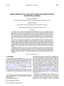
Figure 1: Coleman-Weinberg potential has the true minimum at φ = M . It is flat at the origin φ = 0. Two possibilities of inflationary scenario exist, the large field inflation (chaotic inflation) and the small field inflation (new inflation). The LFI has the beyond-Planck scale problem while the SFI has the fine-tuning problem of the initial condition.

2

Small field inflation and the fine-tuning problem

We particularly consider the CW type potential [12] shown in figure 1;   φ2 1 λφ4 ln 2 − + V0 V (φ) = 4 M 2

(2)

where V0 = λM 4 /8. The minimum of the potential is given at φ = M . In this paper, we assume M  Mpl .

Such potentials are studied in various situations, in particular, in the analysis of the radiative symmetry breaking of gauge theories, such as the grand unified theories (GUT) or extensions of the standard model (SM). Especially, it has attracted renewed interest recently as a simple model of physics beyond the SM satisfying the experimental constraints imposed on the BSM by the LHC and flavor experiments. In [13, 14], based on the idea of [15], we proposed a minimal extension of the SM by introducing B − L (Baryon number minus Lepton number) U (1) gauge field Z 0 , an additional scalar φ whose vacuum expectation value (VEV) breaks the B − L gauge symmetry, and the right handed neutrinos which cancel the gauge anomaly of the B − L symmetry. We show that the electroweak (EW) gauge symmetry breaking is triggered by the B − L breaking, which is radiatively broken by the CW mechanism. The model is a minimal extension of the SM in which radiative symmetry breaking can generate the EW scale. 3

One of our motivations of the present analysis is to investigate the cosmological possibility of the model, but in order to make our discussions as general as possible, we do not use the specific numerical values of the coupling constants in the following. We make use of the scalar field φ as an inflaton field. Since φ has the CW type potential as in the Fig. 1, two types of inflations are possible: the large field inflation (LFI) and the small field inflation (SFI). The large field type can be regarded as the chaotic inflation with a quartic potential. On the other hand, the small field CW inflation was studied in the early eighties in the non-supersymmetric GUT models[16, 17, 18], and called the new inflation. In order to realize the SFI, it is often assumed that the inflaton field is trapped at the origin due to thermal corrections to the effective potential generated in the reheating of the LFI. When the fluctuations of the field are dominated by the vacuum energy at φ = 0, the SFI occurs. Then the radiation generated so far rapidly dilute, and the inflaton field φ rolls down to the true minimum at φ = M . The mechanism works when the reheating occurs by perturbative decay of inflaton. Since the decay process produces relativistic particles, the modification of the inflaton potential is not always sufficient to lift the true minimum to trap the field around the origin. Also, in order to explain the CMB fluctuations, the inflaton field must start from a very small value φ  M near the top of the potential. In the following we explain how much fine-tuning is necessary. First we calculate the slow roll parameters to estimate the necessary initial condition in the SFI. Taking derivatives with respect to φ, we have   φ2 φ2 00 2 0 3 (3) V = λφ ln 2 , V = λφ 2 + 3 ln 2 . M M Mass of the scalar at the minimum is given by m2φ = V 00 (M ) = 2λM 2 . For small values of fields (φ < M ), the slow roll parameters are calculated to be   0 2 2  6  2 2 MPl MPl V φ φ2 ≈ 32  = ln 2 , (4) 2 V M M M  2  2  00  φ2 MPl φ V 2 ≈ 24 ln 2 . (5) η = MPl V M M M Here we used V ≈ V0 in the region φ  M. The slow roll conditions , |η| < 1 require that the field value φ during the SFI must be extremely smaller than M ; thus the relation   |η| follows. Inflation stops at |η| = 1 where the slow roll condition is violated. Eq. (5) can be approximately solved as s   |η| −1 24MP2 l M 2 ln . φ ≈ 24 |η|M 2 Mpl

(6)

It requires that, in order to satisfy the the slow roll condition with sufficiently large e-folding, the inflation must start from the very small initial condition, φini ∼ (10−3 |η|)1/2

M2  M. Mpl

(7)

This is the infamous fine-tuning problem of the initial condition of the SFI. In deriving the coefficient numerically, we inserted M = 1010 GeV and |η| = 0.02 but the coefficient 10−3 does 4

not depend so much on the details of these values. For these values, the initial value needs to be φini ∼ 10−11 M. Since M is the typical scale of the potential (the energy scale at the minimum of the CW potential), such small coefficient 10−11 seems very unnatural as the initial condition. This is one of the reasons that large field inflations, such as the chaotic ones, are more favoured than the SFI. The slow roll parameter  is much smaller than |η| and given by |η|3 = 432 ln(24Mpl2 /|η|M 2 )



M MP l

4

−5

3

∼ 4 × 10 |η|



M MP l

4

1.

(8)

In order to make the amplitude of the scalar perturbation ∆2S consistent with the Planck data [1], ∆2S = 2.215 × 10−9 , the quartic coupling of the CW potential λ must be extremely small λ ∼ 10−15 . In the following sections, we see that the smallness of the coupling becomes important to generate rapid particle creations during coherent oscillations of the inflaton field. Here we comment on the issue of the smallness of the spectral index ns . Those who are more interested in the initial condition problem can skip this paragraph. The e-folding number N of the SFI is related to the slow roll parameter η as   Z φ 1 V 3 1 1 dφ ≈ − . (9) N = 2 0 MPl 2 |η| |ηend | φend V By putting |ηend | = 1, we have η = −1/(2N/3 + 1). Since   |η|, the spectral index of the scalar perturbation is given by ns = 1 − 6 + 2η ∼ 1 + 2η. Hence ns ∼ 0.96 [1] requires an e-folding number N = 3/(1 − ns ) − 3/2 = 73.5. On the other hand, the e-folding number at the pivot scale of CMB is given by !   1/4 1 TR V0 2 + ln , (10) NCMB = 61 + ln 3 1016 GeV 3 1016 GeV where we assumed that there was an epoch of the inflaton field’s oscillation induced by its mass term after the inflation and then the radiation dominated epoch continues until the 1/4 matter-radiation equality epoch. The smallness of the vacuum energy V0 ∼ 10−4 M  MP l suggests a smaller e-folding number than 61, which is inconsistent with the above large e-folding number N = 73.5. Various resolutions of the inconsistency have been proposed [3][4][5]. In our previous letter [6], we proposed another possibility that a linear potential is generated by the chiral condensates of quarks. In the rest of the paper, we solve the fine-tuning problem of the initial condition given in (7) by using the dynamics of preheating during the rapid oscillation of inflaton field before the SFI starts.

3

Large field inflation and beyond-Planck problem

Before trying to solve the initial condition problem of the SFI, we remind the readers of the beyond-Planck scale problem in the LFI. If the inflation has the potential of the CW type in Figure 1, it is natural to think that in the early universe a coherent motion of the inflaton 5

starts from a field value with φ  M. Then the potential can be approximated by the quartic one V = λφ4 /2. The slow roll parameters in the region φ  M are given by  0 2  2 2 V MPl MPl ≈8 (11)  = 2 V φ  2  00  MPl V ≈ 12 = 3/2. (12) η = MPl V φ If the field value is much larger than the Planck scale Mpl , the slow roll conditions are satisfied and the LFI occurs. The spectral index for the scalar perturbation is given by ns = 1−6+2η = 1 − 3. Hence, in order to explain the CMB data ns = 0.9603 ± 0.0073, we need  ∼ 0.013, and accordingly the field value at the pivot scale φ ∼ 25Mpl is necessary. The tensor-scalar ratio is predicted as r = 16 ∼ 0.208, and the e-folding is given by Z φ Z φ V 1 1 1 dφ 2 2 √ √ N = = dφ = (φ − φ ) ∼ −1 end 2 2 0 8MPl  2MPl φend  φend MPl V

(13)

(14)

where we put end = 1. Two drawbacks are known in LFI. First it predicts large tensor to scalar ratio (13) which seems to be inconsistent with the Planck and BICEP2/Keck Array observations [1, 2]. Second the large field value φ  Mpl may invalidate the analysis of the inflaton potential within renormalizable field theories, and higher mass-dimensional terms cannot be excluded. They are common problems of the LFI. We call the second one the beyond-Planck-scale problem in this paper. In the following, we show that, in the CW type potential, the SFI naturally follows the LFI. Hence, the CMB fluctuations are generated during the SFI, and the first problem is absent. Furthermore, as we show later, in order to solve the initial condition problem of the SFI (7), it is sufficient to require that, before the SFI occurs, the field starts from somewhere in an intermediate region M < φ < Mpl . Hence the beyond-Planck-scale problem is also absent.

4

Preheating: broad parametric resonance

We consider a coupled system of two scalar fields, an inflaton field φ and another scalar field χ. The potential of the model is V (φ, χ) = V (φ) +

g2 2 2 φχ , 2

(15)

where V (φ) is given in (2). The model can be considered as a toy model of the classically conformal B − L extended standard model [13]. The SM singlet scalar whose VEV breaks the B − L gauge symmetry plays the role of the inflaton φ, and the scalar field χ corresponds to the B − L U (1) gauge field Z 0 . Hence the coupling g represents the B − L gauge coupling gB−L . In the model [13], Z 0 gauge boson is coupled to the SM particles and decays into them. In the 6

present paper, we briefly comment on the effects of the χ decay and leave detailed (numerical) analysis for future investigations. The strengths of the two coupling constants, λ and g, are assumed to satisfy the following inequality g 2  λ.

(16)

It is a natural assumption since the quartic coupling of the inflaton must be very small λ ∼ 10−15 while the (gauge) coupling g is not necessarily so. The equations of motion of the scalars are given by φ + V 0 (φ) + g 2 χ2 φ = 0, χ + g 2 φ2 χ = 0.

(17)

The d’Alembertian operator acting on modes with comoving momenta k is given by  = ˙ ∂t2 + 3H∂t + (k 2 /a2 ), where a is the scale factor and the Hubble constant is given by H = a/a, " # 2 ˙2 χ ˙ 1 φ H2 = + V (φ, χ) + . (18) 3Mpl2 2 2 We divide the inflaton field into the coherent motion (zero mode) φ0 and fluctuation (non-zero modes) ϕ as φ(t, x) = φ0 (t) + ϕ(t, x) .

(19)

For a sufficiently large initial value φ√ 0 > Mpl , the coherent motion of the inflaton field realizes the LFI. The LFI ends around φ0 ∼ 12Mpl where η ∼ 1, and starts falling down towards the minimum. The energy density of the universe is dominated coherent oscillation, and the √ by the 1 field starts oscillation with the effective frequency ωeff ∼ λΦ0 . Here Φ0 is the amplitude of the oscillation. The effective frequency of the inflaton oscillation ωeff is larger than the Hubble constant H after the oscillation starts. Hence, the expansion of the universe can be neglected during each oscillation of the φ field. It is also worth mentioning here that ωeff largely changes in finite density state. It is discussed in the next section. In the coherent motion of the inflaton field, the χ and the non-zero modes of φ acquire time-dependent mass terms: mχ (t)2 = g 2 φ0 (t)2 ,

mϕ (t)2 = 3λφ0 (t)2 ,

(20)

2 and, if the adiabaticity condition (|ω|/ω ˙ < 1) is violated, particle creations by parametric resonance occur. It is called the preheating mechanism [7]. The equation of motion for the mode with momentum k is approximated by   k2 2 2 2 2 2 2 (21) χ¨k + 3H χ˙ k + ωχ (k)χk ∼ 0 where ωχ (k) = g Φ0 sin (ωeff t) + δm + 2 . a

In √ the quartic potential of λφ4 /4, the solution to the equation of motion φ¨0 + λφ30 = 0 is given by φ0 (t) = Φ0 cn( λΦ0 t, 1/2). The Jacobi √ elliptic function is well approximated by the trigonometric function φ0 (t) ∼ Φ0 cos(ωeff t) where ωeff = 0.8472 λΦ0 . 1

7

For later convenience we added the term δm2 which represents slowly changing mass shifts due to back reactions of the created particles. It is a finite density effect and absent until particles are created by preheating. This term plays an important role in section 5. As mentioned, the expansion of the universe is much slower than the inflaton oscillation. Then, by neglecting the Hubble term, the equation becomes identical with the Mathieu equation. The violation of the adiabaticity condition is efficient near φ0 ∼ 0 and for smaller k. The equation is transformed into the standard form of the Mathieu equation by defining the new coordinate z = ωeff t, ∂ 2 χk + (A − 2q cos 2z)χk = 0, ∂z 2  2  k |mχ |2 (gΦ0 )2 (gΦ0 )2 1 2 , q = = . (22) + δm + A= 2 2 2 ωeff a2 2 4ωeff 4ωeff √ where we defined |mχ | = gΦ0 . In the standard form, A represents the ratio of the (averaged) frequency of the χk field to the frequency of the external force. On the other hand, q represents the strength of the external force. The Mathieu equation describes the phenomena of parametric resonances, and the solution is unstable in some regions of (A, q) parameter space. For q < 1, the solution is unstable only when A satisfies special conditions for the narrow resonance [7]. On the contrary, if the external force is sufficiently strong q > 1, the solution is unstable for wide range of parameter space and the ratio of the frequencies A is not strongly constrained. This is called the broad parametric resonance. In a realistic model, we need to take into account back reactions from the produced particles and the red-shift of momenta by the expansion of the universe. They change the narrow resonance condition for A, and hence, in order to realize the rapid increase of particles due to the Bose enhancement, the broad resonance condition q  1 is necessary. The particle creation is most efficient around φ0 = 0, and in order to estimate the particle creation rate, we expand the external force around φ0 (t) = 0. The equation of motion (21) is then approximated by   2 k 2 2 2 + δm + |ω˙ χ | t χk = 0 . (23) χ¨k + a2

where |ω˙ χ | ≡ gΦ0 ωeff . It is identified with the Schr¨odinger equation in an inverted harmonic potential, and the particle creation due to the Bogoliubov transformation around t = 0 is calculated as the tunneling rate in the potential. The Bogoliubov coefficient βk is given by  2  1 k 2 2 −πκ2k 2 |βk | = e , κk = + δm . (24) |ω˙ χ | a2 A necessary condition for the preheating is κk . 1. Otherwise, the adiabaticity condition is not violated and the particle creations do not occur efficiently. This gives an upper bound of momenta of created particles. To summarize, the particle creation due to the preheating (broad resonance) occurs only when the two conditions, q  1 and κ . 1, are satisfied. For the sufficient particle creation of χ particles, it is necessary to satisfy ·

qχ =

|mχ |2 (gΦ0 )2 g2 = ∼ 1 2 2 4ωeff 4ωeff λ 8

(25)

·

k2 + δm2 . |ω˙ χ | = gΦ0 ωeff a2

(26)

Here we explicitly write the subscript χ in qχ to distinguish it from the same parameter for other particles. When these conditions are satisfied together with the Bose enhancement effect, the rapid growth of the χ particles occur. Then the particle number density increases exponentially as nχ ∝ e2µz . The coefficient µ is O(0.1) [7]. It varies model by model, but the detailed value of µ is not essential in the following discussions. If the created particles χ decay or annihilate into other particles, or dilute due to the rapid expansion of the universe, faster than the creation rate µωeff , Bose enhancement effect does not work. Hence the following conditions ·

µωeff > Γχ , H

(27)

need to be taken into account for the exponential growth of particle The p √ numbers to occur. √ 2 < Hubble parameter H = λ/12(Φ0 /Mpl ) is smaller than µωeff ∼ µ λΦ0 for Φ0 ∼ 12µMpl , and we can neglect the effect of the expansion of the universe in the period of rapid oscillation. In the B − L model [14], χ decays into SM particles with the coupling g. Hence the decay √ 2 3 width √ is given by Γχ ∼ g mχ ∼ g Φ0 while the effective frequency is ωeff ∼ λΦ0 . Hence, if µ λ > g 3 , the condition µωeff > Γχ is satisfied. Indeed, as mentioned at the end of section 7, λ ∼ g 4  1 is required in the model [14] and thus the decay rate is smaller than the production rate. Let’s go back to the conditions (25) and (26) . The first condition (25) is satisfied in our model since λ is extremely small. When δm2 = 0, the second condition (26) gives an upper bound of the physical momenta p = k/a of the created particles, p2 < p2?

(28)

√ p2? ≡ |ω˙ χ | = gΦ0 ωeff ∼ (gΦ0 )2 / qχ .

(29)

where

Since particles with lower momenta are more efficiently produced, the number distribution is far from being in thermal equilibrium. For qχ  1, the mass squared m2χ (t) = (gφ0 (t))2 is larger than p2? and the created χ particles behave non-relativistically, except for short intervals of the −1/4 oscillation satisfying φ0 (t) < qχ gΦ0 . In finite density state discussed in the next section, the l.h.s. of (28) is replaced by p2 + δm2 . Therefore, when back reactions of created particles generate larger mass corrections δm2 > p2? , the wave equations for χ with any low momenta behave adiabatically and the particle creations stop. On the contrary to χ, ϕ particles (non-zero modes of φ) are not efficiently produced by the preheating since the first condition q  1 is not satisfied. The parameter q for ϕ is given by qϕ =

3λΦ20 |mϕ |2 = ∼ O(1) 2 2 4ωeff 4ωeff

(30)

and it does not satisfy the broad resonance condition. Furthermore, as seen in the next section, production of χ particles leads to a larger frequency ωeff , and consequently qϕ becomes much smaller than O(1). Hence the preheating never occurs for ϕ. But instead, ϕ particles can 9

be rapidly produced from the χ particles by rescatterings χ + φ0 → χ + ϕ and annihilations 2χ → φ0 + ϕ, or 2χ → ϕ + ϕ. These particles have momenta p . p? . Since its mass is generated by finite density effects only, ϕ behaves relativistically [20]. It does hold even after the finite density effect gives a nonvanishing mass m2ϕ = λhϕ2 i because λ  g 2 is assumed in the present analysis.

5

Back reactions and the end of preheating

Once the oscillation of the inflaton starts, the number density of χ particles grow exponentially. As discussed, µωeff is much larger than the Hubble constant for Φ0  Mpl , and the production rate of nχ is always larger than the expansion rate of the universe and a precise value of µ is not important. Soon after nχ increases, the scattering and annihilation process through the interaction term g χ φ rapidly create non-zero modes ϕ, and the universe is filled with χ and ϕ particles2 . The number density nϕ grows until it becomes equal to nχ [20]. The χ field acquires an additional mass correction in addition to (20), 2 2 2

m2χ = g 2 (φ20 (t) + hϕ2 i) .

(31)

At the beginning of preheating, the coherent part is dominant, but soon the second term becomes comparable to the first term. The 2-point function at the same space-time point can be evaluated by using the Hartree approximation as Z nϕ d3 k nϕ,k + 1/2 2 ∼ (32) hϕ i = 3 (2πa) ωk p? where ωk is replaced by the typical momentum p? of ϕ. In the following we see that the preheating stops when both terms become comparable and indistinguishable. The coherent motion of φ is also modified by the additional contribution g 2 hχ2 iφ2 /2 in finite density state. The 2-point function for χ field is similarly evaluated as Z d3 k nχ,k + 1/2 nχ 2 hχ i = ∼ . (33) 3 (2πa) ωk g|φ| Here, by using the fact that the created particles are nonrelativistic3 , ωk is replaced by mχ = p g|φ0 (t)|. It is justified as long as |φ0 | > hϕ2 i in (31). Then the interaction between the inflaton and the χ field gives the induced potential which is linear [7] in φ, g 2 2 2 g 2 nχ 2 g hχ iφ ∼ φ = nχ |φ| . 2 2 g|φ| 2 2

(34)

In the paper [20], the evolution of occupation numbers were numerically investigated. FIG.13 in [20] shows the rapid growth of ϕ after χ particles are created by the preheating. It also shows that the occupation numbers of ϕ and χ become equal when the exponential growth stops. 3 At later stages of preheating, the energy is transferred from IR to UV momenta due to scatterings and the χ particles become relativistic. Numerical simulations are necessary for further precise evaluations of hχ2 i. We leave it for future investigations.

10

Comparing this with the original potential λφ4 /2, the above term becomes more dominant when the number of created particles nχ is larger than the number density determined by the amplitude of the inflaton oscillation; nχ > (λ/g)Φ30 . Hence, the quartic potential of the inflaton is gradually modified by the back reaction of created particles, and when the above condition is satisfied, inflaton oscillation can be approximated by the linear-type potential V ∝ |φ| for p 2 |φ| > hϕ i. The effective frequency of the inflaton oscillation in the linear potential is given 2 by ωeff ∼ gnχ /Φ0 ∼ g 2 hχ2 iφ0 =Φ0 . When the 2-point function hϕ2 i in (31) increases up to hϕ2 i = Φ20 , hχ2 i is replaced by hχ2 i =

nχ gΦ0

(35)

and the inflaton potential changes from the linear to the quadratic one for φ < Φ0 ,4 g 2 2 2 gnχ 2 hχ iφ ∼ φ . 2 2Φ0

(36)

Hence the effective frequency of the inflaton oscillation does not changed, and is given by 2 ωeff = gnχ /Φ0 . Through the preheating, the energy of the coherent motion of inflaton is transferred to the energy of the created particles. The preheating finally ends either the condition for the broad parametric resonance qχ > 1 (the value of qχ in zero density state is given in (25)) or the condition for the mass correction δm2 < p2? is violated. Since qχ , δm, p? are functions of g, λ, hχ2 i and hϕ2 i, we need to numerically solve the evolution of 2-point functions hχ2 i, hϕ2 i and the coherent mode Φ0 . In the following we evaluate the conditions for broad parametric resonance based on the above ansatz for the 2-point functions. The parameter qχ gets modifications by the created particles as follows. The mass of the χ field in finite density state is given by eq.(31). On the other hand, the effective frequency ωeff of the inflaton field is given as 2 ωeff ∼ λ(Φ20 + hϕ2 i) + g 2 hχ2 i ,

(37)

and it receives larger corrections than the bare term λΦ20 because λ  g 2 . Accordingly the parameter qχ to determine the broad parametric resonance for χ particles in the finite density state is replaced by m2χ g 2 (Φ20 + hϕ2 i) ∼ . qχ = 2 4ωeff λ(Φ20 + hϕ2 i) + g 2 hχ2 i

(38)

As we saw, when created particles are absent, it is qχ = g 2 /λ  1. As the χ particles are created by preheating (remember g 2  λ), the last term becomes to dominate the denominator 2 and ωeff is approximated by g 2 hχ2 i. The preheating stops when hχ2 i ∼ Φ20 and qχ decreases down to O(1). At the time, the mass of ϕ becomes p mϕ = ωeff ∼ g hχ2 i ∼ gΦ0 . (39) 4

In [11], from the validity of the quadratic potential for φ > Φ0 and numerical simulations, the authors concluded that the effective potential is linear for large φ > Φ0 even after the ϕ production up to hϕ2 i ∼ Φ20 , and consequently the first order phase transition occurs.

11

Thus, since p? =

√

gΦ0 ωeff , we have the following relation mχ ∼ mϕ ∼ p? ∼ gΦ0

(40)

when the preheating stops. If ϕ are rapidly produced by scatterings, we have the chemical equilibrium nϕ ∼ nχ . Then the relation hϕ2 i = hχ2 i = Φ20 follows (32) and (35). This is the case we study in our paper. (See also the footnote 5.) When the condition qχ > 1 is violated, the other condition δm2 < p2? for the preheating becomes simultaneously violated in the above situations. Both sides are given by δm2 = g 2 hϕ2 i p and p2? = gΦ0 ωeff ∼ g 2 Φ0 hχ2 i ∼ g 2 Φ20 . Hence if ϕ particles are rapidly produced and hϕ2 i = hχ2 i = Φ20 holds, δm2 = p2? is satisfied and even zero-momentum particles cannot be created.

To summarize, all the fluctuations have the same amplitude hϕ2 i = hχ2 i = Φ20 when the preheating stops. And the number densities are related to the amplitude of fluctuations as nχ (t) = nϕ (t) = gΦ30 (t) .

(41)

Initially, gΦ30 is larger than nχ and nϕ , and the preheating occurs. The amplitude of the coherent oscillation Φ is reduced and the number density nχ increases. At the same time scatterings produce ϕ particles and increase nϕ . Finally, the preheating stops when the number densities become equal to gΦ30 . In addition, the effective masses of the particles become equal mχ = mϕ = gΦ0 . These properties are consequences of the hierarchy in the coupling constants g 2  λ. The initial value Φ0,start of the coherent motion of the inflaton field determines the amplitude Φ0,end at which the broad parametric resonance stops. Since the particle production occurs faster than the Hubble time scale, the energy conservation gives a relation between them as follows. The potential energy of the initial inflaton configuration λΦ40,start is transfered to the energy of the χ and φ particles ∼ g 2 hϕ2 ihχ2 i = g 2 Φ40,end . Thus we have  1/4 λ Φ0,end = Φ0,start . (42) g2

Note that the finite density state is not in the thermal equilibrium since the preheating is mostly efficient for very low momentum particles. Further studies of the process towards thermal equilibrium (i.e. turbulence flow from IR to UV momenta) are left for future investigations [21] 5 . After the preheating stops, the energy density is dominated by the χ and φ particles, and given by ρ ∼ g 2 Φ40 (t). In the following, we use Φ to indicate the typical amplitude of the fluctuations. As the universe expands, the particle densities gradually dilute and the amplitude Φ(t) decays as well.

6

Trapping the inflaton near the top of the potential

The inflaton potential is modified due to the created particles and the potential is raised, which may prevent the inflaton field from falling down to the minimum φ = M of the Coleman5

In [21], the authors studied a case where the created particles χ interact with themselves and its number density generates the mass for χ itself. In such cases, the exponential growth stops much earlier and the stationary turbulence ( which leads to linear growth of occupation numbers ) is shown to occur. In the process, the energy flows from IR modes to UV modes.

12

1.0

V( )

V( )

0.20

0.8

0.15 0.6

Φ0

0.4

0.10

Φ0

0.2

0.0 0.0

φ 0.2

V( )

0.4

0.6




0.8

1.0

1.2

0.05

φ 0.00 0.0

0.2

V( )

!

"1/3◆ ✓ g 2 g 2 1/3 φ∼ ⇠ Φ0 λ

0.4

0.6

Φ0

0.5

Φ0

1.0

M




1.0

! ✓"1/3 ◆ 2 2 1/3

g g φ∼ ⇠ λ

Φ0




0.8

φ

M

φ




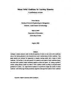
Figure 2: Schematic figures of the inflaton potential modified by the finite density effect. When the amplitude of the fluctuations Φ is larger than Φ1 ≡ (4eλ/3g 2 )1/3 M , the potential has no nontrivial minimum (Fig.A). As the amplitude becomes smaller, the nontrivial minimum appears (Fig.B, C). For smaller amplitude of Φ, the minimum at φ = M becomes the true minimum as in Fig.D. The position of the potential barrier is located around (g 2 /λ)1/3 Φ and it is always on the right of Φ, if g 2 > λ.

Weinberg potential V (φ). Since the magnitude of the potential raise depends on the amplitude of the fluctuations hχ2 i = Φ2 , it is necessary to check whether the field is trapped without falling down to the minimum. In this section, we show that it actually happens for wide range of parameters. As we saw in the previous section, when the number density of created particles becomes comparable to gΦ30 , the preheating stops. After the preheating stops, the amplitudes of fluctuations keep the relation hχ2 i = hϕ2 i = Φ2 since χ and φ particles are in chemical equilibrium and the zero mode φ0 is indistinguishable from the non-zero modes ϕ. Keeping this relation, the amplitudes decrease as the universe expands. When the amplitude of the fluctuations is Φ, the inflaton potential is approximated by ( 2 2   g Φ φ2 1 λ 4 φ2 |φ| < Φ 2 φ ln 2 − + δV, δV = (43) V = 2 3 g Φ 4 M 2 |φ| |φ| > Φ 2 The second term δV is the finite density contribution of created particles. The first term also receives an additional contribution in finite density state, but since g 2 > λ, it is negligible compared to the last term. The main role of the first term is to give the minimum at φ = M. 13

Due to δV , the minimum at φ = M is lifted as in Fig.2. The question is whether the position of the barrier between two minima is on the right of the field value φ = Φ. For g 2 > λ, it can be shown that the modified potential of (43) has a nontrivial minimum only when Φ . Φ1 ≡ (4eλ/3g 2 )1/3 M . Otherwise, the potential has the unique minimum at φ = 0 as in Figure 2A. Thus the coherent motion falls towards the origin until the amplitude becomes smaller than Φ = Φ1 . For Φ < Φ1 in Figure 2B, C, D, the potential has two local minima. It can be easily shown that the position of the barrier between two minima is given by φ ∼ (g 2 /λ)1/3 Φ. Hence, for g 2 > λ, the barrier is always on the right of Φ. Even after the amplitude decreases further and the finite density effect is no longer capable to lift the minimum at φ = M above V = 0 (see Fig.2D ), the inflaton field is kept being trapped within the barrier. The above trapping mechanism occurs only when sufficient particle creation has finished before the field falls down to the true minimum. Namely, in order to trap the field in the potential barrier, the quadratic potential must be generated before the field falls down. A sufficient condition for this is that, the amplitude of the inflaton Φ0,end at the end of the preheating is larger than M ; Φ0,end > M . Therefore, using (42), if Φ0,start satisfies the condition Φ0,start > (g 2 /λ)1/4 M ,

(44)

χ particles are sufficiently produced so that it can trap the inflaton field within the potential barrier.6 The field value Φ0,start can be much smaller than the Planck scale, and the beyondPlanck-scale problem is absent. Finally we comment on the effects of thermalization of χ particles on the trapping mechanism. In particular, we take the B − L model as an example. When the preheating stops, the relation nχ = gΦ3 holds. In the B − L model, as discussed after eq.(27), the decay rate of χ is given by Γχ = g 3 Φ. χ can also annihilate into the SM particles, whose rate is estimated as Γχ,annih ∼ g 4 nχ /m2χ ∼ g 3 Φ. Hence, if Φ < g 2 Mpl , these rates are larger than the Hubble √ parameter H ∼ gΦ2 /Mpl and the thermal bath with the temperature T ∼ gΦ is produced. Furthermore, when Φ < g 7/2 Mpl , the B − L scattering rate satisfies Γscatt ∼ g 4 T > H and all the system including the B − L and the inflaton fields is thermalized. Then the fluctuation of fields are determined by the temperature Φ2T ≡ hϕ2 i ∼ hχ2 i ∼ T 2 ∼ gΦ2 . They are smaller than the original value of the fluctuations hϕ2 i ∼ hχ2 i = Φ2 . This is because thermalization transfers energy from IR to UV regions with typical momentum p ∼ T and reduces the large fluctuation produced by the preheating. Consequently the coefficient of the quadratic term in (43) is replaced by g 2 hχ2 i = g 2 Φ2T for |φ| < ΦT /g. In this case, the position of the barrier is given by (g 2 /λ)1/2 ΦT . For the amplitude of the fluctuation is ΦT , the barrier is always on the right of the fluctuation and the trapping mechanism similarly holds.

7

Dynamical fine-tuning of the initial condition

We now determine the initial value of the SFI. The amplitudes of the oscillation and fluctuations decrease in the expanding universe where the energy density is dominated by the energy of 6

To get the actual lower bound on Φ0,start , accordingly the field value where the zero mode φ0 starts rolling down, we need a detailed numerical calculation with being careful of the shape of the Colman-Weinberg potential (2). It’s beyond the scope of this paper and left as a future work. Depending on the initial value, new inflation with a sufficient e-folding could occur without the inflaton oscillation [19].

14

the created particles, ρ ∼ g 2 Φ4 . But as the amplitude becomes smaller, the vacuum energy V0 = λM 4 /8 will dominate the energy of created particles. By comparing these energies, we see that the de Sitter expansion starts when the amplitude becomes smaller than the following value,  1/4 λ Φ∼ M . (45) 8g 2 It is already small but still much larger than the necessary initial condition in eq.(7). During the de Sitter expansion, the inflaton continues to oscillate until theqeffective frequency of the inflaton ωeff = gΦ becomes smaller than the Hubble constant H = λM 4 /24Mpl2 of the de Sitter universe. Hence the amplitude of fluctuations continues to decay as far as the condition ωeff > H is satisfied. The oscillation of the inflaton finally stops when the condition r 1 λ M2 , (46) Φ. g 24 Mpl is satisfied. After this condition is satisfied, the inequality ωeff < H holds and the fluctuations of the inflaton field with lower momenta than the Hubble constant are frozen. Therefore, in the new inflation model with the Coleman-Weinberg potential, the amplitudes of the coherent motion and also the fluctuations are reduced to the very small value7 . Eq.(46) solves the fine-tuning problem of the small field inflation (7). Let us estimate the coefficient in (46) numerically. The quartic coupling is determined by the amplitude of the curvature fluctuations as λ ∼ 10−15 . Inserting the value in (46), it becomes  −5  2 M 10 −3 . (47) Φ ∼ 10 g Mpl It is smaller than the upper bound of (7) if the coupling g satisfies g & 10−5 . For general models g is a free parameter and we can take any value, but in the B − L extension of the SM [14], the β-function of the quartic coupling λ has a contribution from the gauge coupling; βλ = 96g 4 /16π 2 . Hence unless g 4 ∼ λ, we need a fine-tuning to keep the smallness of λ. The most natural assumption is g ∼ λ1/4 ∼ 10−4 . Thus, within the model [14], the initial condition problem of the SFI is naturally solved.

8

Summary

In this paper, we proposed a mechanism to solve the fine-tuning problem of the new inflation, the small field inflation with the Coleman-Weinberg type potential. The key relation (46) to determine the initial value is obtained by comparing the effective frequency of the oscillation and the Hubble constant (H 2 = V0 /3Mpl2 ). The flatness at the top of the potential is responsible 7

If the system is thermalized as discussed at the end of section 6, the energy density of the universe ρ is given by ∼ Φ4T and the r.h.s. of (45) is replaced by (λ/8)1/4 M . During the de Sitter expansion, the scattering rate Γscatt become smaller than the Hubble constant H. Then the system is no longer in thermal equilibrium. But the amplitude of fluctuation ΦT is red-shifted and continues to reduce as a−1 . Since the effective frequency of inflaton is given by ωeff = gΦT , the fluctuation is frozen at the same value of (46).

15

for the fine-tuning problem of the SFI. Corresponding to this fact, the effective frequency should be dynamically generated by the fluctuations of created particles. Then, from the dimensional analysis, we can expect that it is given by ωeff = gΦ, where g is the coupling to the field which gives effective potential of the inflaton. Then, energy is given by V0 = λM 4 , the √ if the vacuum initial value of the inflaton is given by Φ ∼ λ/g(M 2 /Mpl ). Therefore, once the inflaton field is trapped by the quadratic potential generated in the preheating, the fine-tuning problem in similar models can be solved. For hilltop inflation models with a negative curvature potential (−µ2 φ2 /2) at the origin, the dynamical fine-tuning mechanism for the small field inflation does not work since the system undergoes the first order phase transition before a sufficiently large e-folding number is gained [11]. Hence the flatness (µ = 0) at the top of the hill is essential to solve the fine-tuning problem of the initial condition in SFI. It is interesting that two completely different fine-tuning problems, the Higgs mass [15] and the initial condition in SFI, can be solved dynamically by simply assuming the absence of the dimensionful parameter µ in the bare Lagrangian.

Acknowledgments We would like to thank Hideo Kodama for useful discussions and comments. This work is supported by the Grant-in-Aid for Scientific research from the Ministry of Education, Science, Sports, and Culture, Japan, Nos. 23540329, 23244057 (S.I.), 26105520, 26247042, 15H05889 (K.K.).

References [1] P. A. R. Ade et al. [Planck Collaboration], ”Planck 2015 results. XX. Constraints on inflation,” arXiv:1502.02114[astro-ph.CO]. [2] P. A. R. Ade et al. [BICEP2 and Keck Array Collaborations], “BICEP2 / Keck Array VI: Improved Constraints On Cosmology and Foregrounds When Adding 95 GHz Data From Keck Array,” arXiv:1510.09217 [astro-ph.CO]. [3] G. Barenboim, E. J. Chun and H. M. Lee, “Coleman-Weinberg Inflation in light of Planck,” Phys. Lett. B 730, 81 (2014). [4] K. Nakayama and F. Takahashi, “PeV-scale Supersymmetry from New Inflation,” JCAP 1205, 035 (2012). [5] F. Takahashi, “New inflation in supergravity after Planck and LHC,” Phys. Lett. B 727, 21 (2013) [arXiv:1308.4212 [hep-ph]]. [6] S. Iso, K. Kohri and K. Shimada, “Small field Coleman-Weinberg inflation driven by a fermion condensate,” Phys. Rev. D 91 (2015) 4, 044006 [arXiv:1408.2339 [hep-ph]]. [7] L. Kofman, A. D. Linde and A. A. Starobinsky, “Towards the theory of reheating after inflation,” Phys. Rev. D 56, 3258 (1997) [hep-ph/9704452].

16

[8] P. B. Greene, L. Kofman, A. D. Linde and A. A. Starobinsky, “Structure of resonance in preheating after inflation,” Phys. Rev. D 56, 6175 (1997) [hep-ph/9705347]. [9] L. Kofman, A. D. Linde, X. Liu, A. Maloney, L. McAllister and E. Silverstein, “Beauty is attractive: Moduli trapping at enhanced symmetry points,” JHEP 0405 (2004) 030 [hep-th/0403001]. [10] L. Kofman, A. D. Linde and A. A. Starobinsky, “Nonthermal phase transitions after inflation,” Phys. Rev. Lett. 76 (1996) 1011 [hep-th/9510119]. [11] G. N. Felder, L. Kofman, A. D. Linde and I. Tkachev, “Inflation after preheating,” JHEP 0008 (2000) 010 [hep-ph/0004024]. [12] S. R. Coleman and E. J. Weinberg, “Radiative Corrections As The Origin of Spontaneous Symmetry Breaking,” Phys. Rev. D 7, 1888 (1973). [13] S. Iso, N. Okada and Y. Orikasa, “Classically conformal B − L extended Standard Model,” Phys. Lett. B 676, 81 (2009) “The minimal B − L model naturally realized at TeV scale,” Phys. Rev. D 80, 115007 (2009) [14] S. Iso and Y. Orikasa, “TeV Scale B − L model with a flat Higgs potential at the Planck scale - in view of the hierarchy problem -,” PTEP 2013, 023B08 (2013). [15] W. A. Bardeen, FERMILAB-CONF-95-391-T; H. Aoki and S. Iso, “Revisiting the Naturalness Problem – Who is afraid of quadratic divergences? –,” Phys. Rev. D 86, 013001 (2012); M. Farina, D. Pappadopulo and A. Strumia, “A modified naturalness principle and its experimental tests,” JHEP 1308 (2013) 022; [16] A. D. Linde, “A New Inflationary Universe Scenario: A Possible Solution of the Horizon, Flatness, Homogeneity, Isotropy and Primordial Monopole Problems,” Phys. Lett. B 108, 389 (1982). [17] A. Albrecht and P. J. Steinhardt, “Cosmology for Grand Unified Theories with Radiatively Induced Symmetry Breaking,” Phys. Rev. Lett. 48, 1220 (1982). [18] Q. Shafi and A. Vilenkin, “Inflation with SU(5),” Phys. Rev. Lett. 52, 691 (1984). [19] J. Yokoyama, “Chaotic new inflation and primordial spectrum of adiabatic fluctuations,” Phys. Rev. D59, 107303 (1999). [20] G. N. Felder and L. Kofman, “The Development of equilibrium after preheating,” Phys. Rev. D 63, 103503 (2001) [hep-ph/0011160]. [21] R. Micha and I. I. Tkachev, “Turbulent thermalization,” Phys. Rev. D 70, 043538 (2004) [hep-ph/0403101].

17