Dynamical modelling, identification and software sensors ... - CiteSeerX

Dynamical modelling, identification and software sensors for SBRs H. Fibrianto∗ , D. Mazouni+ , M. Ignatova∗∗ , M. Herveau+ , J. Harmand+ and D. Dochain∗ * : CESAME, Universit´e Catholique de Louvain 4-6 av. Georges Lemaˆıtre, B-1348 Louvain-la-Neuve, Belgium + : LBE-INRA, avenue des ´etangs, F-11100 Narbonne, France ** : ICSR, BAS, P.O.Box 79, 1113 Sofia Bulgaria

1

Introduction

Within the EOLI project, two different types of models have been proposed to represent the dynamics of two different types of processes. These models have been calibrated and validated on experimental data obtained from the different experimental processes. The first model, referred as EM1, corresponds to the process run in Mexico. The second model represent the dynamics of the processes run at POLIMI, at the LBE and at the UU. Due to slight differences between the process dynamics, two submodels have been identified, i.e. EM2a for the POLIMI process, and EM2b for the LBE process. The models as they are presented here are indeed the result of an iterative process between model building and process experiments. If the main frame of the models have been built in the initial step on the basis of the partners’ experience and of the available scientific literature of the subject, several modifications have been included at the light of the physical/(bio)chemical evidences provided by the experiments. This has resulted in the design of extra experiments in order to validate the new modelling assumptions. In this paper, we concentrate on models EM1 and EM2b, which are considered in the second part of the paper for the design of software sensors. Herebelow only the reaction schemes, the mass balance equations (with the kinetic expresssions), the basic identification procedure and the parameter values are provided. Details about the identification procedures for the different models can be found in the related more detailed project reports. The identified models have been used for several purposes in the project : software sensor design, FDI, and control design. In the present manuscript, we concentrate the software sensor design results. As for any biotechnological processes, the on-line monitoring and control of the SBR’s is facing two major difficulties : the lack of measuring devices that can provide the values of all the key process components on-line, and the lack of confidence in the dynamical models of the processes (even with our quite careful identification procedure). This motivates to design software sensors that are capable of providing reliable software measurement (estimates) of the

1

key components in spite of the model uncertainty that is typically mainly concentrated in the process kinetics.

2 2.1

Dynamical models of two SBR’s Model EM1

The process consists of a fed-batch reactor with one single aerobic growth reaction and an endogeneous respiration reaction : Growth : SC + SO −→ X Endogeneous respiration : SO + X −→ X

(1) (2)

where SC , SO and X represent the concentrations of organic matter, dissolved oxygen and biomass, respectively. The dynamics of the process are described by the following equations : dX dt dSC dt dSO dt dV dt

qin X V qin = −k1 µX + (SC,in − SC ) V qin = −k2 µX − bX + (SO,in − SO ) + kL a(SOs − SO ) V = µX −

= qin

(3) (4) (5) (6)

where µ, qin , V , k1 , k2 , b, SC,in , SO,in , kL a and SOs are the specific growth rate, the inlet flow rate, the volume, the yield coefficients (between X and SC , and X and SO ), the endogeneous respiration kinetic constant, the inlet organic matter and dissolved oxygen concentrations, the trnsfer coefficient and the oxygen saturation concentration, respectively. The specific growth rate is represented by the following Haldane model : µ =

µ0 SC S2 KS + S C + C KI

(7)

Since the growth rate of microorganisms is inhibited by the substrate, a fedbatch process operation is particularly adapted in order to continuously maintain the growth rate around its maximum.

2.2

Model EM2b

The process operation consists of two successive batch steps : an anoxic phase followed by an aerobic phase. The model refers explicitely to these two phases. While in EM2a a two step denitrification/nitrification process is considered, in EM2b only one denitrification step and one step nitrification are considered in the anoxic and aerobic phases, respectively [2]. Therefore the reaction scheme considered here is the following. 1. Anoxic phase : denitrification : SC + SN O −→ Xh + N2 2

(8)

2. Aerobic phase : nitrification : SO + SN H −→ Xa + SN O C − removal : SC + SO −→ Xh

(9) (10)

In the above reactions, SN O , Xh , Xa , SN H , hold for the (concentrations of) nitrate + nitrite, the heterotroph and autotroph bacteria and the TKN (Total Kjehdal Nitrogen), respectively. The dynamics are given by the following set of mass balance equations : 1. Anoxic phase dXh = µhN Xh dt dSC = −k1 µhN Xh dt dSN O = −k2 µhN Xh dt

(11) (12) (13)

2. Aerobic phase dXh dt dXa dt dSC dt dSO dt dSN O dt dSN H dt

= µ h Xh

(14)

= µ a Xa

(15)

= −k3 µh Xh

(16)

= −k4 µh Xh − k5 µa Xa + kL a(SOmax − SO )

(17)

= k 6 µ a Xa

(18)

= −k7 µa Xa

(19)

In the oxygen balance equation, the term SOmax accounts for the endogeneous respiration via the following relationship : re SOmax = SOs (20) kL a where re holds for the endogeneous respiration rate (assumed to be (almost) constant). The kinetic expressions are the following : SN O SC − SCmin KC1 + SC − SCmin KN O + SN O SC − SCmin = µhmax SO KCh + SC − SCmin SN H = µamax SO KN Ha + SN H

µhN = µhN max µh µa

(21) (22) (23)

In the above kinetic expressions, the term SCmin accounts for the non-biodegradable part of the organic compound SC . Note also that the specific growth rates in the aerobic phase are proportional to the dissolved oxygen concentration SO in the reactor instead of the classical Monod expression as usually used in Activated Sludge models, e.g. [5]. It is mainly because the available experiments were realized with a non-limiting oxygen concentration. 3

3

Parameter identification of models EM1 and EM2b

The identification of the parameters of both models has been performed as follows ([1], [3]). First experiments have been designed so as to cover a sufficiently wide range of process conditions of interest in order to provide experimental data that can possibly provide a dynamical model structure with parameter values as accurate as possible. The collected data have been distributed in two sets : one for parameter calibration, one for model validation. The identification of the model parameters has been processed so as to estimate the kinetic parameters, the yield coefficients and the transfer coefficients independently of each other. This step is very important to guarantee appropriate and reliable parameter estimation. Moreover confidence intervals for each parameter have been computed. Parameter µ0 KS KI k1 k2 b kL a

Dimension h−1 mg4CP/L mg4CP/L mg4CP/mgV SS mgDO/mgV SS h−1 h−1

Value Confidence interval 0.1916 0.00255 60 0.01499 3.753 0.00755 3.7 1.0363 0.0578 0.0059 0.0004 16.8 0.1

Table 1: Parameter values for model EM1-A3 Parameter k1 k2 µhN max KC1 KN O kL a SOmax k3 k4 k5 k6 k7 µhmax KCh µamax KN Ha SCmin

Dimension mgCOD/mgV SS mgN/mgN min−1 mgCOD/L mgN/L h−1 mg/L mgCOD/mgV SS mgO2 /mgN mgO2 /mgN mgN/mgV SS mgN/mgV SS min−1 mgCOD/L min−1 mgN/L mgCOD/L

Value 0.828 0.905 0.016 144.45 20.47 18.75 7.86 3.38 1.74 7.85 0.28 0.67 0.023 137.6 0.017 95.6 30.42

Table 2: Parameter values for model EM2b for LBE data 4

Different configurations have considered for the parameter calibration (e.g. with or without inlet dissolved oxygen, with or without oxygen sensor dynamics, with or without a modification in the early part of the Haldane kinetics) of model EM1. The following set of parameters (Table 1) correspond to SO,in = 0, SOs = 6 mg/L and no oxygen sensor dynamics. k1 has also been given from separate batch experiments. The identified parameter values from the LBE data for model EM2 are given in Table 2.

4 4.1

Software sensor design Software sensors for EM1

Software sensors are tools that allow to provide on-line values of key process components that are not accessible for on-line measurement. The software sensors for EM1 are concerned with the on-line estimation of substrate and biomass concentrations from the on-line measurements of dissolved oxygen in presence of uncertainty in the kinetics. The design of software sensors has been concentrating on the on-line estimation of biomass and substrate concentrations mainly in the context of the toxic compounds treatment plant described by model EM1 under the assumption (in line with the statistical analysis of the model parameters) of poor knowledge of the kinetics parameters of the biomass growth (Haldane model). The approach considered for the EOLI project for the EM1 model is a combination of an asymptotic observer with an adaptive observer that provides both state and parameter on-line estimates [4]. As a matter of illustration, let us consider the EM1 model where the parameter uncertainty is assumed to be concentrated on the parameter µ0 of the Haldane model. The available on-line measurements are the dissolved oxygen SO and SO,in , the inlet COD concentration SC,in and the inlet flow rate qin . Since the operation time is intrinsically limited, one major challenge in the software sensor design is to be able to act on the convergence rate of the observer so that estimates of the unmeasured biomass and substrate can convergence fast enough to their true experimental values. Asymptotic observers are robust observers with respect to the lack of knowledge about the process kinetics but their convergence rate is fully dependent on the operating conditions (via the inlet flow rate). That’s why an alternative is proposed in the EOLI project that combines an asymptotic observer with an adaptive observer. Let us concentrate here on the case where the priority is to obtain a fast estimate of the biomass concentration X. For the asymptotic observer, we first define the following auxiliary variables : z1 = S O + k 2 X k2 z 2 = S O − SC k1

(24) (25)

Their mass balance equations obtained from model EM1 are equal to : dz1 b = SO − dt k2 b dz2 = SO − dt k2

b z1 + k2 b z1 + k2

qin (SO,in − z1 ) + kL a(SOs − SO ) V qin k2 (SO,in − SC,in − z1 ) + kL a(SOs − SO ) V k1 5

(26) (27)

By inverting the definitions of z1 and z2 , we obtain estimates from the measurement of the dissolved oxygen SO and the values of z1 and z2 provided by the computation of the above equations : Xc =

k1 z1 − S O , SCe = (SO + z2 ) k2 k2

(28)

where SCe and Xe hold for the estimates of SC and X provided by the asymptotic observer. These above 4 equations (26)(27)(28) are the asymptotic observer of our EOLI observer. The adaptive observer is based on the assumption that a mean value of µ0 (denoted µ ¯0 ) is known. The adaptive observer will therefore provide an estimate of the deviation from this mean (possibly wrong) value. The design of the observer is based on the mass balance equations of the biomass concentration X and of the dissolved oxygen concentration SO : ˆ dX ˆ + ∆µ0 φ(SCe )Xe − qin X ˆ + C1 (SO − SˆO ) = µ ¯0 φ(SCe )X (29) dt V dSˆO ˆ − k2 ∆µ0 φ(SCe )Xe − bX ˆ + qin (SO,in − SO ) + kL a(SOs − SO ) = −k2 µ ¯ 0 φ(SCe )X dt V +C2 (SO − SˆO ) (30) d(∆µ0 ) = C3 (SO − SˆO ) (31) dt In the above equations ∆µ0 is the on-line estimate of the deviation of µ0 , and φ(SCe ) is equal to : SCe φ(SCe ) = (32) 2 SCe KS + SCe + KI Note that the estimates of the asymptotic observer are used in the above adaptive observer; they play a key role in the stability analysis of the observer. C1 , C2 and C3 are the design parameters, in other words the knobs on which one can act to modify the convergence rate of the estimation of X. A careful mathematical stability analysis shows that they have to be selected as follows : C1 = −(λ1 + λ2 + λ3 ) −

qin +µ ¯0 φ(SCe ) V

(33)

λ1 λ2 λ3 (34) φ(SCe )Xe (b + k2 qin /V )     λ1 λ2 λ3 qin = −(λ1 λ2 + λ2 λ3 + λ1 λ3 ) + C2 −µ ¯0 φ(SCe ) − C3 k2 φ(SCe )Xe (35) b+µ ¯ 0 φ(SCe ) V

C2 = C3

In the above equations λ1 , λ2 , λ3 are the eigenvalues associated to the adaptive observer. They are indeed the true knobs for selecting the convergence rate. They have to be negative (to guarantee the stability of the adaptive observer). When referring to simple dynamics views, large values of the eigenvalues mean fast convergence. However other dynamical effects (like the zero dynamics) may interfere and deteriorate the convergence in presence of large eigenvalues. Moreover, the presence of noise on the measurement may also limit the values of the eigenvalues. 6

The appropriate selection of the design parameters is therefore a job that has to be performed carefully, in particular via exhaustive numerical simulations. Alternative versions of the above EOLI observer can be deduced, e.g. by considering other parameter uncertainty assumptions or for the on-line estimation of the substrate concentration with convergence faster than with the asymptotic observer. The EOLI observer have been tested in numerical simulation under various conditions. Figure 1 illustrates the performance of the EOLI observer in typical operating conditions of the fedbatch process of Mexico. The intial values of the biomass concentration and of the substrate concentration have been set with 10% error with respect to their values. The eigenvalues have been set to -5. Note that the adaptive observer (dotted line : - -) is able to converge faster to the true value of X (straight line) than the asymptotic observer (dotted line : ...).

X (mgVSS/l)

6000 5000 4000 3000 2000

0

0.5

1

1.5

2

2.5

3

3.5

4

0

0.5

1

1.5

2

2.5

3

3.5

4

0

0.5

1

1.5

2 t (h)

2.5

3

3.5

4

SO (g/l)

6 4 2 0

0

∆ µ (h−1)

0 −0.02 −0.04 −0.06 −0.08

Figure 1: Adaptive observer for the EM1 process

4.2

Software sensors for EM2b

In the present instance, the software sensor design has concentrated in particular on the estimation of the organic matter concentration SC and of the nitrate-nitrite concentrations SN O from the on-line measurements of oxygen SO and of ammonia nitrogen SN H in the aerobic phase [6]. The estimation approach that has been considered here is an asymptotic observer [1]. It is

7

based on the following auxiliary variables z1 and z2 : z1 = S N H +

k7 k4 k5 SN O , z 2 = S O − SC + SN O k6 k3 k6

(36)

whose dynamics are straightforwardly derived from the mass balance equations (14)-(19) : dz1 = 0 dt dz2 = kL a(SOmax − SO ) dt

(37) (38)

The software measurements are given by inverting the defintions of z1 and z2 : k3 k3 k5 SˆC = − (z2 − SO ) + (z1 − SN H ) k4 k4 k7 k6 (z1 − SN H ) SˆN O = k7

(39) (40)

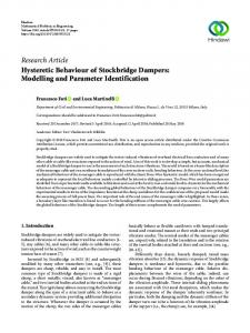
Experimental results for the plant of the LBE-INRA are given on Figure 2.

Figure 2: Asymptotic observer for the EM2b process Note that this estimator requires the knowledge of both Z1 (0) and Z2 (0) in equations (39) and (40). This can be solved as follows. At the beginning of the aerobic phase, there is no 8

nitrite nor nitrate in the reactor. Thus SN O (0) = 0. Since SN H is measured, SN H (0) = SN H0 is known. Since SO is also measured one has only to assume that the initial value of the organic carbon to be removed in one cycle is known (SC (0) = SC0 ). It must then be assumed that an approximate value of SC (0) is known in order to use this estimator. In such a case, the results shown in the figure 2 illustrates the effectiveness of the method. Acknowledgements : This paper includes results of the EOLI project that is supported by the INCO program of the European Community (Contract number ICA4-CT-2002-10012). It also presents research results of the Belgian Programme on Interuniversity Poles of Attraction initiated by the Belgian State, Prime Minister’s Office, Science, Technology and Culture. The scientific responsibility rests with its authors.

References [1] Bastin G. and D. Dochain (1990). On-line Estimation and Adaptive Control of Bioreactors. Elsevier, Amsterdam. [2] Betancur M., D. Dochain and H. Fibrianto (2004). WP 2 : Model Selection and Parameter Identification. EOLI Project, Deliverable D2.3 : Validated Model. [3] Dochain D. and P.A. Vanrolleghem (2001). Dynamical Modelling and Estimation in Wastewater Treatment Processes, IWA Publishing, London. [4] Dochain D. (2003). State observers for processes with uncertain kinetics. International Journal of Control, 76 (15), 1483-1492. [5] Henze, M., C.P.L. Grady, W. Gujer, G.v.R. Marais and T. Matsuo (1987). Activated Sludge Model No.1, IAWPRC Scientific and Technical reports, No.1, IAWPRC, London. [6] Mazouni,D., M. Ignatova and J. Harmand (2005). A multi model approach for the monitoring of carbon and nitrogen concentrations during the aerobic phase of a biological SBR. Proc. IFAC 2005 World Congress, July 4-8, 2005, Prague.

9