The general dynamical sampling problem can be stated as follows: Let f be a function in a separable Hilbert ... For each i â Ω, let Si be the operator from H = l2(I) to Hi = l2({0,...,li}), defined ...... MR 768926 (86h:46001). 16. Bradley Currey and ...
DYNAMICAL SAMPLING A. ALDROUBI, C. CABRELLI, U. MOLTER AND S. TANG Abstract. Let Y = {f (i), Af (i), . . . , Ali f (i) : i ∈ Ω}, where A is a bounded operator on `2 (I). The problem under consideration is to find necessary and sufficient conditions on A, Ω, {li : i ∈ Ω} in order to recover any f ∈ `2 (I) from the measurements Y . This is the so called dynamical sampling problem in which we seek to recover a function f by combining coarse samples of f and its futures states Al f . We completely solve this problem in finite dimensional spaces, and for a large class of self adjoint operators in infinite dimensional spaces. In the latter case, the M¨ untz-Sz´ asz Theorem combined with the Kadison-Singer/Feichtinger Theorem allows us to show that Y can never be a Riesz basis when Ω is finite. We can also show that, when Ω is finite, Y = {f (i), Af (i), . . . , Ali f (i) : i ∈ Ω} is not a frame except for some very special cases. The existence of these special cases is derived from Carleson’s Theorem for interpolating sequences in the Hardy space H 2 (D).
1. Introduction Dynamical sampling refers to the process that results from sampling an evolving signal f at various times and asks the question: when do coarse samplings taken at varying times contain the same information as a finer sampling taken at the earliest time? In other words, under what conditions on an evolving system, can time samples be traded for spatial samples? Because dynamical sampling uses samples from varying time levels for a single reconstruction, it departs from classical sampling theory in which a signal f does not evolve in time and is to be reconstructed from its samples at a single time t = 0, see [1, 2, 5, 7, 8, 11, 19, 20, 28, 23, 30, 33, 37, 43, 44, and references therein]. The general dynamical sampling problem can be stated as follows: Let f be a function in a separable Hilbert space H, e.g., Cd or `2 (N), and assume that f evolves through an evolution operator A : H → H so that the function at time n has evolved to become f (n) = An f . We identify H with `2 (I) where I = {1, . . . , d} in the finite dimensional case, I = N in the infinite dimensional case. We denote by {ei }i∈I the standard basis of `2 (I). The time-space sample at time t ∈ N and location p ∈ I, is the value At f (p). In this way we associate to each pair (p, t) ∈ I × N a sample value. Date: September 29, 2014. 2010 Mathematics Subject Classification. 94O20, 42C15, 46N99. Key words and phrases. Sampling Theory, Frames, Sub-Sampling, Reconstruction, M¨ untz-Sz´ asz Theorem, Feichtinger conjecture, Carleson’s Theorem . The research of A. Aldroubi and S. Tang is supported in part by NSF Grant DMS- 1322099. C. Cabrelli and U. Molter are partially supported by Grants PICT 2011-0436 (ANPCyT), PIP 2008-398 (CONICET) and UBACyT 20020100100502 and 20020100100638 (UBA). . 1
2
A. ALDROUBI, C. CABRELLI, U. MOLTER, S. TANG
The general dynamical sampling problem can then be described as: Under what conditions on the operator A, and a set S ⊆ I × N, can every f in the Hilbert space H be recovered in a stable way from the samples in S. At time t = n, we sample f at the locations Ωn ⊆ I resulting in the measurements {f (n) (i) : i ∈ Ωn }. Here f (n) (i) =< An f, ei > . The measurements {f (0) (i) : i ∈ Ω0 } that we have from our original signal f = f (0) will contain in general insufficient information to recover f . In other words, f is undersampled. So we will need some extra information from the iterations of f by the operator A: {f (n) (i) = An f (i) : i ∈ Ωn }. Again, for each n, the measurements {f (n) (i) : i ∈ Ωn } that we have by sampling our signals An f at Ωn are insufficient to recover An f in general. Several questions arise. Will the combined measurements {f (n) (i) : i ∈ Ωn } contain in general all the information needed to recover f (and hence An f )? How many iterations L will we need (i.e., n = 1, . . . , L) to recover the original signal? What are the right “spatial” sampling sets Ωn we need to choose in order to recover f ? In what way all these questions depend on the operator A? The goal of this paper is to answer these questions and understand completely this problem that we can formulate as: Let A be the evolution operator acting in `2 (I), Ω ⊆ I a fixed set of locations, and {li : i ∈ Ω} where li is a positive integer or +∞. Problem 1.1. Find conditions on A, Ω and {li : i ∈ Ω} such that any vector f ∈ `2 (I) can be recovered from the samples Y = {f (i), Af (i), . . . , Ali f (i) : i ∈ Ω} in a stable way. Note that, in Problem 1.1, we allow li to be finite or infinite. Note also that, Problem 1.1 is not the most general problem since the way it is stated implies that Ω = Ω0 and Ωn = {i ∈ Ω0 : li ≥ n}. Thus, an underlying assumption is that Ωn+1 ⊆ Ωn for all n ≥ 0. For each i ∈ Ω, let Si be the operator from H = `2 (I) to Hi = `2 ({0, . . . , li }), defined by Si f = (Aj f (i))j=0,...,li and define S to be the operator S = S0 ⊕ S1 ⊕ . . . Then f can be recovered from Y = {f (i), Af (i), . . . , Ali f (i) : i ∈ Ω} in a stable way if and only if there exist constants c1 , c2 > 0 such that c1 kf k22 ≤ kSf k22 =
X
kSi f k22 ≤ c2 kf k22 .
(1)
i∈Ω
Using the standard basis {ei } for `2 (I), we obtain from (1) that c1 kf k22 ≤
li XX
|hf, A∗j ei i|2 ≤ c2 kf k22 .
i∈Ω j=0
Thus we get Lemma 1.2. Every f ∈ `2 (I) can be recovered from the measurements set Y = {f (i), Af (i), . . . , Ali f : i ∈ Ω} in a stable way if and only if the set of vectors {A∗j ei : i ∈ Ω, j = 0, . . . , li } is a frame for `2 (I). 1.1. Connections to other fields. The dynamical sampling problem has similarities to other areas of mathematics. For example, in wavelet theory [9, 16, 17, 25, 34, 38, 42], a high-pass convolution operator H and a low-pass convolution operator
DYNAMICAL SAMPLING
3
L are applied to the function f . The goal is to design operators H and L so that reconstruction of f from samples of Hf and Lf is feasible. In dynamical sampling there is only one operator A, and it is applied iteratively to the function f . Furthermore, the operator A may be high-pass, low-pass, or neither and is given in the problem formulation, not designed. In inverse problems (see [36] and the references therein), a single operator B, that often represents a physical process, is to be inverted. The goal is to recover a function f from the observation Bf . If B is not bounded below, the problem is considered an ill-posed inverse problem. Dynamical sampling is different because An f is not necessarily known for any n; instead f is to be recovered from partial knowledge of An f for many values of n. In fact, the dynamical sampling problem can be phrased as an inverse problem when the operator B is the operation of applying the operators A, A2 , . . . , AL and then subsampling each of these signals accordingly on some sets Ωn for times t = n. The methods that we develop for studying the dynamical sampling problem are related to methods in spectral theory, operator algebras, and frame theory [2, 10, 13, 15, 18, 20, 21, 22, 45]. For example, the proof of our Theorems 3.9 and 3.13, below, use the newly proved [35] Kadison-Singer/Feichtinger conjecture [14, 12]. Another example is the existence of cyclic vectors that form frames, which is related to Carleson’s Theorem for interpolating sequences in the Hardy space H 2 (D) (c.f., Theorem 3.14). Application to Wireless Sensor Networks (WSN) is a natural setting for dynamical sampling. In WSN, large amounts of physical sensors are distributed to gather information about a field to be monitored, such as temperature, pressure, or pollution. WSN are used in many industries, including the health, military, and environmental industries (c.f., [29, 31, 39, 32, 41, 40] and the reference therein). The goal is to exploit the evolutionary structure and the placement of sensors to reconstruct an unknown field. The idea is simple. If it is not possible to place sampling devices at the desired locations, then we may be able to recover the desired information by placing the sensors elsewhere and use the evolution process to recover the signals at the relevant locations. In addition, if the cost of a sensor is expensive relative to the cost of activating the sensor, then, we may be able to recover the same information with fewer sensors, each being activated more frequently. In this way, reconstruction of a signal becomes cheaper. In other words we perform a time-space trade-off. 1.2. Contribution and organization. In section 2 we present the results for the finite dimensional case. Specifically, Subsection 2.1 concerns the special case of diagonalizable operators acting on vectors in Cd . This case is treated first in order to give some intuition about the general theory. For example, Theorem 2.2 explains the reconstruction properties for the examples below: Consider the following two matrices acting on C5 . P =
9/2 1/2 −7 5 −3 15/2 3/2 −11 5 −7 5 0 −7 5 −5 4 0 −4 3 −4 1/2 1/2 −1 0 1
Q=
3/2 −1/2 2 0 1 1/2 5/2 0 0 −1 0 0 3 0 0 . 1 0 −1 3 −1 −1/2 −1/2 1 0 3
4
A. ALDROUBI, C. CABRELLI, U. MOLTER, S. TANG
For the matrix P , Theorem 2.2 shows that any f ∈ C5 can be recovered from the data sampled at the single “spacial” point i = 2, i.e., from Y = {f (2), P f (2), P 2 f (2), P 3 f (2), P 4 f (2)}. However, if i = 3, i.e., Y = {f (3), P f (3), P 2 f (3), P 3 f (3), P 4 f (3)} the information is not sufficient to determine f . In fact if we do not sample at i = 1, or i = 2, the only way to recover any f ∈ C5 is to sample at all the remaining “spacial” points i = 3, 4, 5. For example, Y = {f (i), P f (i) : i = 3, 4, 5} is enough data to recover f , but Y = {f (i), P f (i), ..., P L f (i) : i = 3, 4}, is not enough information no matter how large L is. For the matrix Q, Theorem 2.2 implies that it is not possible to reconstruct f ∈ C5 if the number of sampling points is less than 3. However, we can reconstruct any f ∈ C5 from the data Y ={f (1), Qf (1), Q2 f (1), Q3 f (1), Q4 f (1), f (2), Qf (2), Q2 f (2), Q3 f (2), Q4 f (2), f (4), Qf (4)}. Yet, it is not possible to recover f from the set Y = {Ql f (i) : i = 1, 2, 3, l = 0, . . . , L} for any L. Theorem 2.2 gives all the sets Ω such that any f ∈ C5 can be recovered from Y = {Al f (i) : i ∈ Ω, l = 0, ...li }. In subsection 2.2 Problem 1.1 is solved for the general case in Cd , and Corollary 2.7 elucidates the example below: Consider
R=
0 −1 4 −1 2 2 1 −2 1 −2 −1/2 −1/2 3 0 1 . 1/2 −1/2 0 2 0 −1/2 −1/2 2 −1 2
Then, Corollary 2.7 shows that Ω must contain at least two “spacial” sampling points for the recovery of functions from their time-space samples to be feasible. For example, if Ω = {1, 3}, then Y = {Rl f (i) : i ∈ Ω, l = 0, . . . , L} is enough recover f ∈ C5 . However, if Ω is changed to Ω = {1, 2}, then Y = {Rl f (i) : i ∈ Ω, l = 0, . . . , L} does not provide enough information. The dynamical sampling problem in infinite dimensional separable Hilbert spaces is studied in Section 3. For this case, we restrict ourselves to certain classes of self adjoint operators in `2 (N). In light of Lemma 1.2, in Subsection 3.1, we characterize the sets Ω ⊆ N such that FΩ = {Aj ei : i ∈ Ω, j = 0, . . . , li } is complete in `2 (N) (Theorem 3.2). However, using the newly proved [28] Kadison-Singer/Feichtinger conjecture [11, 9], we also show that if Ω is a finite set, then {Aj ei : i ∈ Ω, j = 0, . . . , li } is never a basis (see Theorem 3.7). It turns out that the obstruction to being a basis is redundancy. This fact is proved using the beautiful M¨ untz-Sz´asz Theorem 3.4 below. Although FΩ = {Aj ei : i ∈ Ω, j = 0, . . . , li } cannot be a basis, it should be possible that FΩ is a frame for sets Ω ⊆ N with finite cardinality. It turns out however, that except for special cases, if Ω is a finite set, then FΩ is not a frame for `2 (N).
DYNAMICAL SAMPLING
5
If Ω consists of a single vector, we are able to characterize completely when FΩ is a frame for `2 (N) (Theorem 3.14), by relating our problem to a theorem by Carleson on interpolating sequences in the Hardy spaces H 2 (D). 2. Finite dimensional case In this section we will address the finite dimensional case. That is, our evolution operator is a matrix A acting on the space Cd and I = {1, . . . , d}. Thus, given A, our goal is to find necessary and sufficient conditions on the set of indices Ω ⊆ I and the numbers {li }i∈Ω such that every vector f ∈ Cd can be recovered from the samples {Aj f (i) : i ∈ Ω, j = 0, . . . , li } or equivalently (using Lemma 1.2), the set of vectors {A∗j ei : i ∈ Ω, j = 0, . . . , li } is a frame of Cd .
(2)
(Note that this implies that we need at least d space-time samples to be able to recover the vector f ). The problem can be further reduced as follows: Let B be any invertible matrix with complex coefficients, and let Q be the matrix Q = BA∗ B −1 , so that A∗ = B −1 QB. Let bi denote the ith column of B. Since a frame is transformed to a frame by invertible linear operators, condition (2) is equivalent to {Qj bi : i ∈ Ω, j = 0, . . . , li } being a frame of Cd . This allows us to replace the general matrix A∗ by a possibly simpler matrix and we have: Lemma 2.1. Every f ∈ Cd can be recovered from the measurement set Y = {Aj f (i) : i ∈ Ω, j = 0, . . . , li } if and only if the set of vectors {Qj bi : i ∈ Ω, j = 0, . . . , li } is a frame for Cd . We begin with the simpler case when A∗ is a diagonalizable matrix. 2.1. Diagonalizable Transformations. Let A ∈ Cd×d be a matrix that can be written as A∗ = B −1 DB where D is a diagonal matrix of the form λ1 I1 0 ··· 0 λ I 2 2 ··· D = .. .. .. . . . 0 0 ···
0 0 .. .
.
(3)
λ n In
In (3), Ik is an hk × hk identity matrix, and B ∈ Cd×d is an invertible matrix. Thus A∗ is a diagonalizable matrix with distinct eigenvalues {λ1 , . . . , λn }. Using Lemma 2.1 and Q = D, Problem 1.1 becomes the problem of finding necessary and sufficient conditions on vectors bi and numbers li , and the set Ω ⊆ {1, . . . , m} such that the set of vectors {Dj bi : i ∈ Ω, j = 0, . . . , li } is a frame for Cd . Recall that the Q-annihilator qbQ of a vector b is the monic polynomial of smallest degree, such that qbQ (Q)b ≡ 0. Let Pj denote the orthogonal projection in Cd onto the eigenspace of D associated to the eigenvalue λj . Then we have: Theorem 2.2. Let Ω ⊆ {1, . . . , d} and let {bi : i ∈ Ω} be vectors in Cd . Let ri be the degree of the D-annihilator of bi and let li = ri − 1. Then {Dj bi : i ∈ Ω, j =
6
A. ALDROUBI, C. CABRELLI, U. MOLTER, S. TANG
0, . . . , li } is a frame of Cd if and only if {Pj (bi ) : i ∈ Ω} form a frame of Pj (Cd ), j = 1, . . . , n. As a corollary, using Lemma 2.1 we get Theorem 2.3. Let A∗ = B −1 DB, and let {bi : i ∈ Ω} be the column vectors of B whose indices belong to Ω. Let ri be the degree of the D-annihilator of bi and let li = ri − 1. Then {A∗j ei : i ∈ Ω, j = 0, . . . , li } is a frame of Cd if and only if {Pj (bi ) : i ∈ Ω} form a frame of Pj (Cd ), j = 1, . . . , n. Equivalently, any vector f ∈ Cd can be recovered from the samples Y = {f (i), Af (i), . . . , Ali f (i) : i ∈ Ω} if and only if {Pj (bi ) : i ∈ Ω} form a frame of Pj (Cd ), j = 1, . . . , n. Note that, in the previous Theorem, the number of time-samples li depends on the sampling point i. If instead the number of time-samples L is the same for all i ∈ Ω, (note that L ≥ max{li : i ∈ Ω} is an obvious choice, but depending on the vectors bi it may be possible to choose L ≤ min{li : i ∈ Ω}), then we have the following Theorems (see Figures 1) Theorem 2.4. Let Ω ⊆ {1, . . . , d} and {bi : i ∈ Ω} be a set of vectors in Cd such that {Pj (bi ) : i ∈ Ω} form a frame of Pj (Cd ), j = 1, . . . , n. Let L be any S fixed integer, then E = {bi , Dbi , . . . , DL bi } is a frame of Cd if and only if {i∈Ω:bi 6=0}
{DL+1 bi , :
i ∈ Ω} ⊆ span(E).
As a corollary, for our original problem 1.1 we get Theorem 2.5. Let A∗ = B −1 DB, L be any fixed integer, and let {bi : i ∈ Ω} be a set of vectors in Cd such that {Pj (bi ) : i ∈ Ω} form a frame of Pj (Cd ), j = 1, . . . , n. Then {A∗j ei : i ∈ Ω, j = 0, . . . , L} is �a frame of Cd if and only if {DL+1 bi : i ∈ Ω} ⊆ span {Dj bi : i ∈ Ω , j = 0, . . . , L} . Equivalently any f ∈ Cd can be recovered from the samples Y = {f (i), Af (i), A2 f (i), . . . , AL f (i) : i ∈ Ω}, if and only if {DL+1 bi : i ∈ Ω} ⊆ span {Dj bi : i ∈ Ω , j = 0, . . . , L} . �
Examples where L < d, while li = d for all i ∈ Ω can be found in [3]. Theorems 2.3 and 2.5 will be consequences of our general results but we state them here to help the comprehension of the general results below. 2.2. General linear transformations. For a general matrix we will need to use the reduction to its Jordan form. To state our results in this case, we need to introduce some notations and describe the general Jordan form of a matrix with complex entries. (For these and other results about matrix or linear transformation decompositions see for example [27].) A matrix J is in Jordan form if J1 0 · · · 0 J2 · · · J = .. .. . . . . . 0 0 ···
0 0 . .. .
Jn
(4)
DYNAMICAL SAMPLING
7
Figure 1. Illustration of a time-space sampling pattern. Crosses correspond to time-space sampling points. Left panel: Ω = Ω0 = {1, 4, 5}. l1 = 1, l4 = 4, l5 = 3. Right panel: Ω = Ω0 = {1, 4}. L = 4. In (4), for s = 1, . . . , n, Js = λs Is + Ns where Is is an hs × hs identity matrix, and Ns is a hs × hs nilpotent block-matrix of the form: Ns1 0 ··· 0 N s2 · · · Ns = .. . .. .. . . 0 0 ···
0 0 .. .
where each Nsi is a
tsi
×
tsi
(5)
Nsγs
cyclic nilpotent matrix,
s
s
Nsi ∈ Cti ×ti ,
0 0 0 1 0 0 0 1 0 Nsi = . . . . .. . . . 0 0 0
··· ··· ··· .. . ···
0 0 0 0 0 0 , .. .. . . 1 0
(6)
with ts1 ≥ ts2 ≥ . . . , and ts1 + ts2 + · · · + tsγs = hs . Also h1 + · · · + hn = d. The matrix J has d rows and distinct eigenvalues λj , j = 1, . . . , n. Let kjs denote the index corresponding to the first row of the block Nsj from the matrix J, and let ekjs be the corresponding element of the standard basis of Cd . (That is a cyclic vector associated to that block). We also define Ws := span{ekjs : j = 1, . . . , γs }, for s = 1, . . . , n, and Ps will again denote the orthogonal projection onto Ws . Finally, recall that the J annihilator qbJ of a vector b is the monic polynomial of smallest degree, such that qbJ (J)b ≡ 0. Using the notations and definitions above we can state the following theorem: Theorem 2.6. Let J be a matrix in Jordan form, as in (4). Let Ω ⊆ {1, . . . , d} and {bi : i ∈ Ω} be a subset of vectors of Cd , ri be the degree of the J-annihilator of the vector bi and let li = ri − 1. Then the following propositions are equivalent. i) The set of vectors {J j bi : i ∈ Ω, j = 0, . . . , li } is a frame for Cd . ii) For every s = 1, . . . , n, {Ps (bi ), i ∈ Ω} form a frame of Ws .
8
A. ALDROUBI, C. CABRELLI, U. MOLTER, S. TANG
Now, for a general matrix A, using Lemma 2.1 we can state: Corollary 2.7. Let A be a matrix, such that A∗ = B −1 JB, where J ∈ Cd×d is the Jordan matrix for A∗ . Let {bi : i ∈ Ω} be a subset of the column vectors of B, ri be the degree of the J-annihilator of the vector bi , and let li = ri − 1. Then, every f ∈ Cd can be recovered from the measurement set Y = {(Aj f )(i) : i ∈ Ω, j = 0, . . . , li } of Cd if and only if {Ps (bi ), i ∈ Ω} form a frame of Ws . In other words, we will be able to recover f from the measurements Y , if and only if the Jordan-vectors of A∗ (i.e. the columns of the matrix B that reduces A∗ to its Jordan form) corresponding to Ω satisfy that their projections on the spaces Ws form a frame. Remark 2.8. We want to emphasize at this point, that given a matrix in Jordan form there is an obvious choice of vectors in order that their iterations give a frame of the space, (namely, the cyclic vectors ekjs corresponding to each block). However, we are dealing here with a much more difficult problem. The vectors bi are given beforehand, and we need to find conditions in order to decide if their iterations form a frame. The following theorem is just a statement about replacing the optimal iteration of each vector bi by any fixed number of iterations. The idea is, that we iterate a fixed number of times L but we do not need to know the degree ri of the J-annihilator for each bi . Clearly, if L ≥ max{ri − 1 : i ∈ Ω} then we can always recover any f from Y . But the number of time iterations L may be smaller than any ri − 1, i ∈ Ω. In fact, for practical purposes it might be better to iterate, than to try to figure out which is the degree of the annihilator for bi . Theorem 2.9. Let J ∈ Cd×d be a matrix in Jordan form (see (4)). Let Ω ⊆ {1, . . . , d}, and let {bi : i ∈ Ω} be a set of vectors in Cd , such that for each s = 1, . . . , n the projections {Ps (bi ) : i ∈ Ω} onto Ws form a frame of Ws . Let L be any S fixed integer, then E = {bi , Jbi , . . . , J L bi } is a frame of Cd if and only if {i∈Ω:bi 6=0}
{J L+1 bi : i ∈ Ω} ⊆ span(E). As a corollary we immediately get the solution to Problem 1.1 in finite dimensions. Corollary 2.10. Let Ω ⊆ I, A∗ = B −1 JB, and L be any fixed integer. Assume that {Ps (bi ) : i ∈ Ω} form a frame of Ws and set E = {J s bi : i ∈ Ω, s = 0, . . . , L, }. Then any f ∈ Cd can be recovered from the samples Y = {f (i), Af (i), A2 f (i), . . . , AL f (i) : i ∈ Ω}, if and only if {J L+1 bi : i ∈ Ω} ⊆ span(E}). 2.3. Proofs. In order to introduce some needed notations, we first recall the standard decomposition of a linear transformation acting on a finite dimensional vector space that produces a basis for the Jordan form. Let V be a finite dimensional vector space of dimension d over C and let T : V −→ V be a linear transformation. The characteristic polynomial of T factorizes as χT (x) = (x−λ1 )h1 . . . (x−λn )hn where hi ≥ 1 and λ1 , . . . , λn are distinct elements of C. The minimal polynomial of T will be then mT (x) = (x − λ1 )r1 . . . (x − λn )rn with 1 ≤ ri ≤ hi for i = 1, . . . , n. By the primary decomposition theorem, the
DYNAMICAL SAMPLING
9
subspaces Vs = Ker(T − λs I)rs , s = 1, . . . , n are invariant under T (i.e. T (Vs ) ⊆ Vs ) and we have also that V = V1 ⊕ · · · ⊕ Vn . Let Ts be the restriction of T to Vs . Then, the minimal polynomial of Ts is (x − λs )rs , and Ts = Ns + λs Is , where Ns is nilpotent of order rs and Is is the identity operator on Vs . Now for each s we apply the cyclic decomposition to Ns and the space Vs to obtain: Vs = Vs1 ⊕ · · · ⊕ Vsγs where each Vsj is invariant under Ns , and the restriction operator Nsj of Ns to Vsj is a cyclic nilpotent operator on Vsj . Finally, let us fix for each j a cyclic vector wsj ∈ Vsj and define the subspace Ws = span{ws1 . . . wsγs }, W = W1 ⊕ · · · ⊕ Wn and let PWs be the projection onto Ws , with IW = PW1 + · · · + PWn . With this notation we can state the main theorem of this section: Theorem 2.11. Let {bi : i ∈ Ω} be a set of vectors in V . If the set {PWs bi : i ∈ Ω} is complete in Ws for each s = 1, . . . , n, then the set {bi , T bi , . . . , T li bi : i ∈ Ω} is a frame of V , where ri is the degree of the T -annihilator of bi and li = ri − 1. To prove Theorem 2.11, we will first concentrate on the case where the transformation T has minimal polynomial consisting of a unique factor, i.e. mT (x) = (x − λ)r , so that T = λId + N , and N r = 0 but N r−1 6= 0. 2.4. Case T = λId + N . Remark 2.12. It is not difficult to see that, in this case, given some L ∈ N, {T j bi : i ∈ Ω, j = 0, . . . , L} is a frame for V if and only if {N j bi : i ∈ Ω, j = 0, . . . , L} is a frame for V . In addition, since N r bi = 0 we need only to iterate to r − 1. In fact, we only need to iterate each bi to li = ri − 1 where ri is the degree of the N annihilator of bi . Definition 2.13. A matrix A ∈ Cd×d is perfect if aii 6= 0, i = 1, . . . , d and det(Ai ) 6= 0, i = 1, . . . , d where As ∈ Cs×s is the submatrix of A, As = {ai,j }i,j=1,...,s . We need the following lemma that is straightforward to prove. Lemma 2.14. Let A ∈ Cd×d be an invertible matrix. Then there exists a perfect matrix B ∈ Cd×d that consists of row (or column) permutations of A. If N is nilpotent of order r, then there exist γ ∈ N and invariant subspaces Vi ⊆ V , i = 1, . . . , γ such that V = V1 ⊕ · · · ⊕ Vγ ,
dim(Vj ) = tj , tj ≥ tj+1 , j = 1, . . . , γ − 1,
and N = N1 + · · · + Nγ , where Nj = Pj N Pj is a cyclic nilpotent operator in Vj , j = 1, . . . , γ. Here Pj is the projection onto Vj . Note that t1 + · · · + tγ = d. For each j = 1, . . . , γ, let wj ∈ Vj be a cyclic vector for Nj . Note that the set {w1 , . . . , wγ } is a linearly independent set. Let W = span{w1 , . . . , wγ }. Then, we can write V = W ⊕ N W ⊕ · · · ⊕ N r−1 W . P Furthermore, the projections PN j W satisfy PN2 j W = PN j W , and I = r−1 j=0 PN j W . Finally, note that N s PW = PN s W N s . (7) With the notation above, we have the following theorem:
10
A. ALDROUBI, C. CABRELLI, U. MOLTER, S. TANG
Theorem 2.15. Let N be a nilpotent operator on V . Let B ⊆ V be a finite set of vectors such that {PW (b) : b ∈ B} is complete in W . Then [ n
o
b, N b, . . . , N lb b
is a frame for V,
b∈B
where lb = rb − 1 and rb is the degree of the N -annihilator of b. Proof. In order to prove Theorem 2.15, we will show that there exist vectors {b1 , . . . , bγ } in B, where γ = dim(W ), such that γ n [
bi , N bi , . . . , N ti −1 bi
o
is a basis of V.
i=1
Recall that ti are the dimensions of Vi defined above. Since {PW (b) : b ∈ B} is complete in W and dim(W ) = γ it is clear that we can choose {b1 , . . . , bγ } ⊆ B such that {PW (bi ) : i = 1, . . . , γ} is a basis of W . Since {w1 , . . . , wγ } is also a basis of W , there exist unique scalars {θi,j : i, j = 1, . . . , γ} such that, PW (bi ) =
γ X
θij wj .
(8)
j=1
with the matrix Θ = {θi,j }i,j=1,...,γ invertible. Thus, using Lemma 2.14 we can relabel the indices of {bi } in such a way that Θ is perfect. Therefore, without loss of generality, we can assume that {b1 , . . . , bγ } are already in the right order, so that Θ is perfect. � We will now prove that the d vectors bi , N bi , . . . , N ti −1 bi i=1,...,γ are linearly independent. For this, assume that there exist scalars αjs such that 0=
γ X j=1
αj0 bj +
p1 X
pr−1
αj1 N bj + · · · +
j=1
X
αjr−1 N r−1 bj ,
(9)
j=1
where ps = max{j : tj > s} = dimN s W, s = 1, . . . , r − 1 (note that ps ≥ 1, since N r−1 b1 6= 0). Note that since V = W ⊕N W ⊕· · ·⊕N r−1 W , for any vector x ∈ V , PW (N x) = 0. Therefore, if we apply PW on both sides of (9), we obtain γ X
αj0 PW bj = 0.
j=1
Since {PW bi : i = 1, . . . , γ} are linearly independent, we have αj0 = 0, j = 1, . . . , γ. Hence, if we now apply PN W to (9), we have as before that p1 X
αj1 PN W N bj = 0.
j=1
Using the conmutation property of the projection, (7), we have p1 X j=1
αj1 N PW bj = 0.
DYNAMICAL SAMPLING
11
In matrix notation, this is N w1 .. 1 1 [α1 . . . αp1 ]Θp1 = 0. . N wp1
Note that by definition of p1 , N w1 , . . . , N wp1 span N W , and since the dimension of N W is exactly p1 , N w1 , . . . , N wp1 are linearly independent vectors. Therefore [α11 . . . αp11 ]Θp1 = 0. Since Θ is perfect, [α11 . . . αp11 ] = [0 . . . 0]. Iterating the above argument, the Theorem follows. � Proof of Theorem 2.11 . We will prove the case when the minimal polynomial has only two factors. The general case follows by induction. That is, let T : V → V be a linear transformation with characteristic polynomial of the form χT (x) = (x − λ1 )h1 (x − λ2 )h2 . Thus, V = V1 ⊕ V2 where V1 , V2 are the subspaces associated to each factor, and T = T1 ⊕ T2 . In addition, W = W1 ⊕ W2 where W1 , W2 are the subspaces of the cyclic vectors from the cyclic decomposition of N1 with respect of V1 and of N2 with respect to V2 . Let {bi : i ∈ Ω} be vectors in V that satisfy the hypothesis of the Theorem. For each bi we write bi = ci + di with ci ∈ V1 and di ∈ V2 , i ∈ Ω. Let ri , mi and ni be the degrees of the annihilators qbTi , qcTi1 and qdTi2 , respectively. By hypothesis {PW1 ci : i ∈ Ω} and {PW2 di : i ∈ Ω} are complete in W1 and W2 , respectively. Hence, applying S Theorem 2.15 to N1 and N2 we conclude that i∈Ω {T1j ci , j = 0, 1, . . . mi − 1} is S complete in V1 , and that i∈Ω {T2j di , j = 0, 1, . . . ni − 1} is complete in V2 . We will now need a Lemma: (Recall that qbT is the T -annihilator of the vector b) Lemma 2.16. Let T be as above, and V = V1 ⊕ V2 . Given b ∈ V , b = c + d then qbT = qcT1 qdT2 where qcT1 and qdT2 are coprime. Further let u ∈ V2 , u = qcT1 (T2 )d. Then quT2 coincides with qdT2 . Proof. The fact that qbT = qcT1 qdT2 with coprime qcT1 and qdT2 is a consequence of the decomposition of T . Now, by definition of quT2 we have that 0 = quT2 (T2 )(u) = quT2 (T2 )(qcT1 (T2 )d) = (quT2 qcT1 )(T2 )d. Thus, qdT2 has to divide quT2 · qcT1 , but since qdT2 is coprime with qcT1 , we conclude that qdT2
divides
quT2 .
(10)
On the other hand 0 = qdT2 (T2 )(d) = qcT1 (T2 )(qdT2 (T2 )d) = (qcT1 qdT2 )(T2 )d = (qdT2 qcT1 )(T2 )d = qdT2 (T2 )(qcT1 (T2 )d) = qdT2 (T2 )(u), and therefore quT2
divides
From (10) and (11) we obtain qdT2 = quT2 .
qdT2 .
(11) �
12
A. ALDROUBI, C. CABRELLI, U. MOLTER, S. TANG
Now, we continue with the proof of the Theorem. Recall ri , mi and ni be the degrees of qbTi , qcTi1 and qdTi2 , respectively, and let li = ri − 1. Also note that by Lemma 2.16 ri = mi + ni . In order to prove that the set {bi , T bi , . . . , T li bi : i ∈ Ω} is complete in V, we will replace this set with a new one in such a way that the dimension of the span does not change. For each i ∈ Ω, let ui = qcTi1 (T2 )di . Now, for a fixed i we leave the vectors bi , T bi , . . . , T mi −1 bi unchanged, but for s = 0, . . . , ni − 1 we replace the vectors T mi +s bi by the vectors T mi +s bi + βs (T )bi where βs is the polynomial βs (x) = xs qcTi1 (x) − xmi +s . Note that span{bi , T bi , . . . , T mi +s bi } remains unchanged, since βs (T )bi is a linear combination of the vectors {T s bi , . . . , T mi +s−1 bi }. Now we observe that: h
i
h
i
T mi +s bi + βs (T )bi = T1mi +s ci + βs (T1 )ci + T2mi +s di + βs (T2 )di . The first term of the sum on the right hand side of the equation above is in V1 and the second in V2 . By definition of βs we have: T1mi +s ci + βs (T1 )ci = T1mi +s ci + T1s qcTi1 (T1 )ci − T1mi +s ci = T1s qcTi1 (T1 )ci = 0, and T2mi +s di + βs (T2 )di = T2s qcTi1 (T2 )(di ) = T2s ui . Thus, for each i ∈ Ω, the vectors {bi , . . . , T li bi } have been replaced by the vectors {bi , . . . , T mi −1 bi , ui , . . . , T ni −1 ui } and both sets have the same span. To finish the proof we only need to show that the new system is complete in V . Using Lemma 2.16, we have that for each i ∈ Ω, dim(span{ui , . . . , T2ni −1 ui }) = dim(span{di , . . . , T2ni −1 di }) = ni , and since each T2s ui ∈ span{di , . . . , T2ni −1 di } we conclude that span{ui , . . . , T2ni −1 ui : i ∈ Ω} = span{di , . . . , T2ni −1 di : i ∈ Ω}.
(12)
Now assume that x ∈ V with x = x1 + x2 , xi ∈ Vi . Since by hypothesis span{ci , . . . , T1mi −1 ci : i ∈ Ω} is complete in V1 , we can write x1 =
i −1 X mX
αji T1j ci ,
(13)
i∈Ω j=0
for same scalars αji , and therefore, i −1 X mX
αji T j bi = x1 +
i∈Ω j=0
i −1 X mX
αji T2j di = x1 + x ˜2 ,
(14)
i∈Ω j=0
i j i −1 since i∈Ω m ˜2 is in V2 by the invariance of V2 by T . Since by j=0 αj T2 di = x j hypothesis {T2 di : i ∈ Ω, j = 1, . . . , ni − 1} is complete in V2 , by equation (12), {T2j ui : i ∈ Ω, j = 1, . . . , ni − 1} is also complete in V2 , and therefore there exist scalars βji ,
P
P
x2 − x ˜2 =
i −1 X nX
i∈Ω j=0
βji T2j ui ,
DYNAMICAL SAMPLING
13
and so x=
i −1 X mX
αji T j bi +
i∈Ω j=0
i −1 X nX
βji T2j ui ,
i∈Ω j=0
which completes the proof of Theorem 2.11 for the case of two coprime factors in the minimal polynomial of J. The general case of more factors follows by induction adapting the previous argument. � Theorem 2.6 and Theorem 2.9 and its corollaries are easy consequences of Theorem 2.11. Proof of Theorem 2.9. Note that if {J L+1 bi : i ∈ Ω} ⊆ span(E), then {J L+2 bi : i ∈ Ω} ⊆ span(E) as well. Continuing in this way, it follows that for each i ∈ Ω, span(E) contains all the powers J j bi for any j. Therefore, using Theorem 2.6, it follows that span(E) contains a frame of Cd , so that, span(E) = Cd and E is a frame of Cd . The converse is obvious. � The proof of Theorem 2.5 uses a similar argument. Although Theorem 2.2 is a direct consequence of Theorem 2.6, we will give a simpler proof for this case. Proof of Theorem 2.2. Let {Pj (bi ) : i ∈ Ω} form a frame of Pj (Cd ), for each j = 1, . . . , n. Since we are working with finite dimensional spaces, to show that {Dj bi : i ∈ Ω, j = 0, . . . , li } is a frame of Cd , all we need to show is that it is complete in Cd . Let x be any vector in Cd , then x =
n P
Pj x. Assume that hDl bi , xi = 0 for all i ∈ Ω and l = 0, . . . , li .
j=1
Since li = ri − 1, where ri is the degree of the D-annihilator of bi , we have that hDl bi , xi = 0 for all i ∈ Ω and l = 0, . . . , d. In particular, since n ≤ d, hDl bi , xi = 0 for all i ∈ Ω and l = 0, . . . , n. Then hDl bi , xi =
n X
hDl bi , Pj xi =
j=1
n X
λlj hPj bi , Pj xi = 0,
(15)
j=1
for all i ∈ Ω and l = 0, . . . , n. Let zi be the vector hPj bi , Pj xi ∈ Cn . Then for each i, (15) can be written in matrix form as V zi = 0 where V is the n × n Vandermonde matrix 1 1 ··· 1 λ1 λ2 · · · λn V = .. (16) .. .. , . . . . . . �
λn−1 λn−1 ··· 1 2
λnn−1
which is invertible since, by assumption, the λj s are distinct. Thus, zi = 0. Hence, for each j, we have that hPj bi , Pj xi = 0 for all i ∈ Ω. Since {Pj (bi ) : i ∈ Ω} form a frame of Pj (Cd ), Pj x = 0. Hence, Pj x = 0 for j = 1, . . . , n and therefore x = 0. �
14
A. ALDROUBI, C. CABRELLI, U. MOLTER, S. TANG
2.5. Remark. Given a general linear transformation T : V −→ V , the cyclic decomposition theorem gives the rational form for the matrix of T in some special basis. A natural question is then if we can obtain a similar result to Theorem 2.11 for this decomposition. (Rational form instead of Jordan form). The answer is no. That is, if a set of vectors bi with i ∈ Ω where Ω is a finite subset of {1, . . . , d} when projected onto the subspace generated by the cyclic vectors, is complete in this subspace, this does not necessarily imply that its iterations T j bi are complete in V . The following example illustrates this fact for a single cyclic operator. • Let T be the linear transformation in R3 given as multiplication by the following matrix M. 0 0 1 M = 1 0 1 0 1 2 The matrix M is in rational form with just one cyclic block. The vector e1 = (1, 0, 0) is cyclic for M . However it is easy to see that there exists a x1 vector b = x2 in R3 such that PW (b) = x1 6= 0, (here W is span{e1 }), x3 but {b, M b, M 2 b} are linearly dependent, and hence do not span R3 . So our proof for the Jordan form uses the fact that the cyclic components in the Jordan decomposition are nilpotent! 3. Dynamical Sampling in infinite dimensions In this section we consider the dynamical sampling problem in a separable Hilbert space H, that without any lost of generality we can consider to be `2 (N). The evolution operators we will consider belong to the following class A of bounded self adjoint operators: A = {A ∈ B(`2 (N)) : A = A∗ , and there exists a basis of `2 (N) of eigenvectors of A}. The notation B(H) stands for the bounded linear operators on the Hilbert space H. So, if A ∈ A there exists an unitary operator B such that A = B ∗ DB with P D = j λj Pj with pure spectrum σp (A) = {λj : j ∈ N} ⊆ R and orthogonal P projections {Pj } such that j Pj = I and Pj Pk = 0 for j 6= k. Note that the class A includes all the bounded self-adjoint compact operators. Remark 3.1. Note that by the definition of A, we have that for any f ∈ `2 (N) and l = 0, . . . < f, Al ej >=< f, B ∗ Dl Bej >=< Bf, Dl bj >
and
kAl k = kDl k.
It follows that FΩ = Al ei : i ∈ Ω, l = 0, . . . , li is complete, (minimal, frame) if � and only if Dl bi : i ∈ Ω, l = 0, . . . , li is complete (minimal, frame). �
3.1. Completeness. In this section, we characterize the sampling sets Ω ⊆ N such that a function f ∈ `2 (N) can be recovered from the data Y = {f (i), Af (i), A2 f (i), . . . , Ali f (i) : i ∈ Ω} where A ∈ A, and 0 ≤ li ≤ ∞.
DYNAMICAL SAMPLING
15
For each set Ω we consider the set of vectors OΩ := {bj = Bej : j ∈ Ω}, where ej is the jth canonical vector of `2 (N). For each bi ∈ OΩ we define ri to be the degree of the D-annihilator of bi if such annihilator exists, or we set ri = ∞. This number ri is also the degree of the A-annihilator of ei . for the remainder of this paper we let li = ri − 1. Theorem 3.2. Let A ∈ A and Ω ⊆ N. Then the set FΩ = Al ei : i ∈ Ω, l = � 0, . . . , li is complete in `2 (N) if and only if for each j, the set Pj (bi ) : i ∈ Ω is complete on the range Ej of Pj . In particular, f is determined uniquely from the set �
Y = {f (i), Af (i), A2 f (i), . . . , Ali f (i) : i ∈ Ω} �
if and only if for each j, the set Pj (bi ) : i ∈ Ω is complete in the range Ej of Pj . Remarks 3.3. i) Note that Theorem 3.2 implies that |Ω| ≥ supj dim(Ej ). Thus, if any eigen-space has infinite dimensions, it is necessary to have infinitely many “spacial” sampling points in order to recover f . ii) Theorem 3.2 can be extended to a larger class of operators. For example, for the class of operators Ae in B(`2 (N)) in which A ∈ Ae if A = B −1 DB where with P D = j λj Pj with pure spectrum σp (A) = {λj : j ∈ N} ⊆ C and orthogonal P projections {Pj } such that j Pj = I and Pj Pk = 0 for j 6= k. Proof of Theorem 3.2. � By Remark 3.1, to prove the theorem we only need to show that Dl bi : i ∈ Ω, l = � 0, . . . , li is complete if and only if for each j, the set Pj (bi ) : i ∈ Ω is complete in the range Ej of P . �j l Assume that D bi : i ∈ Ω, l = 0, . . . , li is complete. For a fixed j, let g ∈ Ej and assume that < g, Pj bi >= 0 for all i ∈ Ω. Then for any l = 0, 1, . . . , li , we have λl < g, Pj bi >=< g, λl Pj bi >=< g, Pj Dl bi >=< g, Dl bi >= 0. � Since Dl bi : i ∈ Ω, l = 0, . . . , li is complete in `2 (N), g = 0. It follows that � Pj (bi ) : i ∈ Ω is complete on the range Ej of Pj . � Now assume that Pj (bi ) : i ∈ Ω is complete in the range Ej of Pj . Let S = � l
span D bi ; i ∈ Ω, l = 0, . . . , li . Clearly DS ⊆ S. Thus S is invariant for D. Since D is self-adjoint, S ⊥ is also invariant for D.PIt follows that the orthogonal projection PS ⊥ commutes with D. Hence, PS ⊥ = j Pj PS ⊥P Pj where convergence is in the strong operator topology. In particular PS ⊥ bi = j Pj PS ⊥ Pj bi = 0. Multiplying both sides by the projection Pk for some fixed k we get that Pk PS ⊥ Pk bi = Pk PS ⊥ Pk (Pk bi ) = 0. �
Since Pk (bi ) : i ∈ Ω is complete in Ek and since k was arbitrary, it follows that Pk PS ⊥ Pk = 0 for each k. Hence PS ⊥ = 0. That is FΩ is complete which finishes the proof of the theorem. � 3.2. Minimality and bases for the dynamical sampling in infinite dimensional Hilbert spaces. � In this section we will show, that for any Ω ⊆ N, the set FΩ = Al ei : i ∈ Ω, l = 0, . . . , li is never minimal if Ω is a finite set, and hence the set FΩ is never a basis.
16
A. ALDROUBI, C. CABRELLI, U. MOLTER, S. TANG
In some sense, the set FΩ contains many ”redundant vectors” which prevents it from being a basis. However, when FΩ is complete, this redundancy may help FΩ to be a frame. We will discuss this issue in the next section. For this section, we need the celebrated M¨ untz-Sz´ asz Theorem characterizing the sequences of monomials that are complete in C[0, 1] or C[a, b] [24]: Theorem 3.4 (M¨ untz-Sz´ asz Theorem). Let 0 ≤ n1 ≤ n2 ≤ . . . be an increasing sequence of nonnegative integers. Then (1) {xnk } is complete in C[0, 1] if and only if n1 = 0 and
∞ P
1/nk = ∞.
k=2
(2) If 0 < a < b < ∞, then {xnk } is complete in C[a, b] if and only if ∞.
∞ P
1/nk =
k=2
We are now ready to state the main results of this section. Theorem 3.5. Let A ∈ A and let Ω be a non-empty subset of N. If there exists bi ∈ OΩ such that ri = ∞, then the set FΩ is not minimal. As an immediate corollary we get Theorem 3.6. Let A ∈ A and let Ω be a finite subset of N. If FΩ = Al ei : i ∈ Ω, l = 0, . . . , li is complete in `2 (N), then FΩ is not minimal in `2 (N). �
Another immediate corollary is Theorem 3.7. Let A ∈ A and let Ω be a finite subset of N. Then the set FΩ = � l A ei : i ∈ Ω, l = 0, . . . , li is not a basis for `2 (N). Remarks 3.8. (1) Theorem 3.7 remains true for the class of operators A ∈ Ae described in Remark 3.3. (2) Theorems 3.6 and 3.7 do not hold in the case of Ω being an infinite set. A trivial example is when A = I is the identity matrix and Ω = N. A less trivial example is when B ∈ `2 (Z) is the symmetric bi-infinite matrix with entries Bii = 1, Bi(i+1) = 1/4 and Bi(i+k) = 0 for k ≥ 2. Let Ω = 3Z and Dkk = 2 if k� = 3Z, Dkk = 1 if k = 3Z + 1, and Dkk = −1 if k = 3Z + 2. Then FΩ = Al ei : i ∈ Ω, l = 0, . . . , 2 is a basis for `2 (Z). In fact FΩ is a Riesz basis of `2 (Z). Examples in which the Ω is nonuniform can be found in [4]. Proof of Theorem 3.5. Again, using Remark 3.1, we will show that {Dl b : l = 0, 1, . . . } is not minimal. P We first assume that D = j λj Pj is non-negative, i.e., λj ≥ 0 for all j ∈ N. Since A ∈ B(`2 (N)), we also have that 0 ≤ λj ≤ kDk < ∞. Let b ∈ OΩ with r = ∞ and f ∈ span{Dl b : l = 0, 1, . . . } be a fixed vector. Let nk be any increasing sequence of nonnegative integers such that
∞ P
1/nk = ∞. Then for any � > 0, there exists a
k=2 − p(D)bk2 ≤
polynomial p such that kf �/2. Since the polynomial p is a continuous function on C[0, kDk], (by the M¨ untz-Sz´asz Theorem) there exists a function g ∈
DYNAMICAL SAMPLING
17
span{1, xnk : k ∈ N} such that sup |p(x) − g(x)| : x ∈ [0, kDk] ≤ �
� 2kbk2 .
Hence
kf − g(D)bk2 ≤ kf − p(D)bk2 + kp(D)b − g(D)bk2 � � ≤ + kbk2 = �. 2 2kbk2 Therefore span{b, Dnk b : k ∈ N} = span{Dl b : l = 0, 1, . . . } and we conclude that {Dl b : l = 0, 1, . . . } is not minimal. P If the assumption about the non-negativity of D = j λj Pj is removed, then by the previous argument {D2l b : l = 0, 1, . . . } is not minimal hence {Dl b : l = 0, 1, . . . } is not minimal either, and the proof is complete. � 3.3. Frames in infinite dimensional Hilbert spaces. � In the previous sections, we have seen that although the set FΩ = Al ei : i ∈ Ω, l = 0, . . . , li is complete for appropriate sets Ω, it cannot form a basis for `2 (N) if Ω is a finite set, in general. The main reason is that FΩ cannot be minimal, which is necessary to be a basis. On the other hand, the non-minimality is a statement about redundancy. Thus, although FΩ cannot be a basis, it is possible that FΩ is a frame for sets Ω ⊆ N with finite cardinality. Being a frame is in fact desirable since in this case we can reconstruct any f ∈ `2 (N) in stable way from the data Y = {f (i), Af (i), A2 f (i), . . . , Ali f (i) : i ∈ Ω}. In this section we will show that, except for some special case of the eigenvalues of A, if Ω is a finite set, i.e., |Ω| < ∞, then FΩ can never be a frame for `2 (N). Thus essentially, either the eigenvalues of A are nice as we will make precise below and even a single element set Ω and its iterations may be a frame, or, the only hope for FΩ to be be a frame for `2 (N) is that Ω infinite - moreover, it need to be well-spread over N. Theorem 3.9. Let A ∈ A and let Ω ⊆ N be a finite subset of N. If FΩ = Al ei : i ∈ Ω, l = 0, . . . , li is a frame, then �
inf{kAl ei k2 : i ∈ Ω, l = 0, . . . , li } = 0. Proof of Theorem 3.9. If FΩ is a frame, then it is complete. Thus the set Ω∞ := {i ∈ Ω : li = ∞} is nonempty since |Ω| < ∞. In addition, if FΩ is a frame, then it is a Bessel sequence. Hence sup{k(D)l bi k2 = kAl ei k2 : i ∈ Ω, l = 0, . . . , li } ≤ C2 for some C2 < ∞. If inf{kAl ei k2 : i ∈ Ω, l = 0, . . . , li } = 6 0, then the set {k(D)l bi k2 = kAl ei k2 : i ∈ Ω, l = 0, . . . , li } is also bounded below by some positive constant C1 . Therefore, the Kadison-Singer/Feichtinger conjectures proved recently [35] applies, and FΩ is the finite union of Riesz sequences
N S j=1
Rj . Let i0 ∈ Ω∞ . Consider the subset {(D2 )l bi0 :
l = 0, . . . , ∞}. Then (by Remark 3.1) each set {(D2 )l bi0 : l = 0, . . . , ∞} ∩ Rj is a Riesz sequence as well (i.e., a Riesz basis of the closure of its span). Thus, there exists an increasing sequence {nk } with
∞ P 1 2 nk nk = ∞ and j0 such that {(D ) bi0 :
k=2
k = 1, . . . , ∞} is a subset of Rj0 . Hence {(D2 )nk bi0 : k = 1, . . . , ∞} is a basis of span{(D2 )nk bi0 : k = 1, . . . , ∞}. Note that σ(D2 ) ⊆ [0, kDk2 ]. Now using the M¨ untz-Sz´ asz Theorem 3.4 it follows {(D2 )nk bi0 : k = 1, . . . , ∞} is not minimal and
18
A. ALDROUBI, C. CABRELLI, U. MOLTER, S. TANG
hence is not a basis for the closure of its span which is a contradiction. Thus, inf{kAl ei k2 : i ∈ Ω, l = 0, . . . , li } = 0. � Therefore, when |Ω| < ∞, the only possibility for FΩ to be a frame, is that inf{kAl ei k2 : i ∈ Ω, l = 0, . . . , li } = 0 and sup{kAl ei k2 : i ∈ Ω, l = 0, . . . , li } ≤ C2 < ∞. We have the following theorem to establish for which finite sets Ω, FΩ is not a frame for `2 (N). Theorem 3.10. Let A ∈ A and let Ω ⊆ N be�a finite subset of N. If 1 or −1 is(are) not a cluster point(s) of σ(A), then FΩ = Al ei : i ∈ Ω, l = 0, . . . , li is not a frame. As an immediate corollary we get Corollary 3.11.� Let A be a compact self-adjoint operator, and Ω ⊆ N be a finite set. Then FΩ = Al ei : i ∈ Ω, l = 0, . . . , li is not a frame. e Remark 3.12. Theorems 3.9 and 3.10 can be generalized for the class A ∈ A.
Proof of Theorem 3.10. If FΩ is not complete, then it is obviously not a frame of `2 (N). If FΩ is complete in `2 (N), then the set Ω∞ := {i ∈ Ω : li = ∞} is nonempty. If there exists j ∈ N and i ∈ Ω∞ such that |λj | ≥ 1 and Pj bi 6= 0 then for x = Pj bi we have X X |hx, Dl bi i|2 = |λj |2l kPj bi k42 = ∞. l
l
Thus, FΩ is not a frame. Otherwise, let r = sup{|λj | : Pj bi 6= 0 for some i ∈ Ω∞ } < 1. j∈N
Since −1 or 1 are not cluster points of σ(A), r < 1. But kDbi k2 ≤ sup{|λj | : Pj bi 6= 0}kbi k2
∀i ∈ Ω∞ ,
j∈N
and therefore we have that kDl bi k2 ≤ rl kbi k2 . Now given � > 0, there exists N such that X X kDl bi k22 ≤ �. i∈Ω∞ l>N
Choose f ∈ `2 (N) such that kf k2 = 1, < f, Dl bi >= 0 for all i ∈ Ω − Ω∞ and l = 0, . . . , li and such that < f, Dl bi >= 0 for all i ∈ Ω∞ and l = 0, . . . , N . Then li XX
| < f, Dl bi > |2 ≤ � = �kf k2 .
i∈Ω l=0
Since � is arbitrary, the last inequality implies that FΩ is not a frame since it cannot have a positive lower frame bound. � Although Theorem 3.10 states that FΩ is not a frame for `2 (N), it could be that after normalization of the vectors in FΩ , the new set ZΩ is a frame for `2 (N). It turns out that the obstruction is intrinsic. In fact, this case is even worse, since ZΩ is not a frame even if 1 or −1 is (are) a cluster point(s) of σ(A).
DYNAMICAL SAMPLING
19
Theorem 3.13. Let A ∈ A and let Ω ⊆ N be a finite set. Then the unit norm � l sequence kAAl eeik2 : i ∈ Ω, l = 0, . . . , li is not a frame. i
Proof. Note that by Remark 3.1,
� Al e i
kAl ei k2
l
: i ∈ Ω, l = 0, . . . , li is a frame if and
only if ZΩ = kDDl bbik2 : i ∈ Ω, l = 0, . . . , li is a frame. i Now, using the exact same argument as for Theorem 3.9 we obtain the desired result. � �
We will now concentrate on the case where there is a cluster point of σ(A) at 1 or −1, and we start with the case where Ω consists of a single sampling point. Since A ∈ A, A = B ∗ DB, by Remark 3.1 FΩ is a frame of `2 (N) if and only if there exists a vector b = Bej for some j ∈ N that corresponds to the sampling point, and {Dl b : l = 0, . . . } is a frame for `2 (N). For this case, Theorem 3.2 implies that if FΩ is a frame of `2 (N), then the projection operators Pj used in the description of the operator A ∈ A must be of rank 1. Moreover, the vector b corresponding to the sampling point must have infinite support, otherwise lb < ∞ and FΩ cannot be complete in `2 (N). Moreover, for this case in order for FΩ to be a frame, it is necessary that |λk | < 1 for all k, otherwise, if there exists λj0 ≥ 1 then for x = Pj0 b (note that by Theorem 3.2 Pj0 b 6= 0) we would have X X |hx, Dn bi|2 = |λj0 |2n kPj0 bk42 = ∞, n
n
which is a contradiction. In addition, if FΩ is a frame, then the sequence {λk } cannot have a cluster point a with |a| < 1. To see this, suppose there is a subsequence λks → a for some a P with |a| < 1, and let W = s Pks (`2 (N)). Then W and W ⊥ are invariant for D, and `2 (N) = W ⊕ W ⊥ . Set D1 = D|W , and b1 = PW b where PW is the orthogonal projection on W . Then, by Theorem 3.10, {D1j b1 : j = 0, 1, . . . } can not be a frame for W . It follows that FΩ cannot be a frame for `2 (N) = W ⊕ W ⊥ . Thus the only possibility for FΩ to be a frame of `2 (N) is that |λk | → 1. These remarks allow us to characterize when FΩ is a frame for the situation when |Ω| = 1. Theorem 3.14. Let D = j λj Pj be such that Pj have rank 1 for all j ∈ N, and let b ∈ `2 (N). Then {Dl b : l = 0, 1, . . . } is a frame if and only if i) |λk | < 1 for all k. ii) |λk | → 1. iii) {λk } satisfies Carleson’s condition P
inf n
Y |λn − λk | k6=n
¯ n λk | |1 − λ
≥ δ.
(17)
for some p δ > 0. iv) bk = mk 1 − |λk |2 for some sequence {mk } satisfying 0 < C1 ≤ |mk | ≤ C2 < ∞. This theorem implies the following Corollary: Corollary 3.15. Let A = B ∗ DB ∈ A, and D = j λj Pj be such that Pj have rank 1 for all j ∈ N. Then, there exists i0 ∈ N such that FΩ = {Al ei0 : l = 0, . . . } is a P
20
A. ALDROUBI, C. CABRELLI, U. MOLTER, S. TANG
frame for `2 (N), if and only if {λj } satisfy the conditions of Theorem 3.14 and there exists i0 ∈ N, such that b = Bei0 satisfies the condition iv of Theorem 3.14 . Theorem 3.14 follows from the discussion above and the following two Lemmas Lemma 3.14 and assume that |λk | < 1 for all k. Let p 3.16. Let D be as in Theorem 0 0 2 bk = 1 − |λk | , and assume that b ∈ `2 (N). Let b ∈ `2 (N). Then, {Dl b : l ∈ N} is a frame for `2 (N ) if and only if {Dl b0 : l ∈ N} is a frame and there exist C1 and C2 such that bk /b0k = mk satisfies 0 < C1 ≤ |mk | ≤ C2 < ∞. Note that by assumption |λk | → 1.
P∞
k=1 (1
− |λk |2 ) < +∞ since b0 ∈ `2 (N). In particular
Lemma 3.17. Let D = j λj Pj be such that |λk | < 1, λk −→ 1 and let b0k = p 1 − |λk |2 . Then the following are equivalent: i) {b0 , Db0 , D2 b0 , . . . } is a frame for `2 (N ) ii) Y |λn − λk | inf ≥ δ. ¯ n λk | n |1 − λ k6=n P
for some δ > 0. In Lemma 3.17, the assumption λk −→ 1 can be replaced by λk −→ −1 and the lemma remains true. Its proof, below, is due to J. Antezana [6] and is a consequence of a theorem by Carleson [26] about interpolating sequences in the Hardy space H 2 (D) of the unit disk in C. Proof of Lemma 3.16. Let us first prove the sufficiency. Assume that {Dl b0 : l ∈ N} is a frame for 2 ` (N) with positive frame bounds A, B, and let b ∈ `2 (N) such that bk = mk b0k with 0 < C1 ≤ |mk | ≤ C2 < ∞. Let x ∈ `2 (N) be an arbitrary vector and define yk = mk xk . Then y ∈ `2 (N) and C1 kxk2 ≤ kyk ≤ C2 kxk2 . Hence C12 Akxk22 ≤
X
|hy, Dl b0 i|2 =
l
X
hx, Dl bi|2 ≤ C22 Bkxk22 ,
l
{Dl b
`2 (N).
and therefore : l ∈ N} is a frame for Conversely, let b ∈ `2 (N) and assume that {Dl b : l ∈ N} is a frame for `2 (N ) with frame bounds A0 and B 0 . Then for any vector ek of the standard orthonormal basis of `2 (N), we have 0
A ≤ √
√
∞ X
| < ek , Dl b > |2 =
l=0
Thus A0 b0k ≤ |bk | √ ≤ B 0 b0k for all √ k. 0 bk = mk bk satisfies A0 ≤ |mk | ≤ B 0 . Let x ∈ `2 (N) be an arbitrary vector and
|bk |2 ≤ B0. 1 − |λk |2
Thus, the sequence {mk } ⊆ C defined by and define now yk =
1 m k xk .
Then y ∈ `2 (N)
X X A0 B0 2 l 0 2 l 2 kxk ≤ |hx, D b i| = |hy, D bi| ≤ kxk22 . 2 0 B0 A l l
and so {Dl b0 : l ∈ N} is a frame for `2 (N).
�
DYNAMICAL SAMPLING
21
The proof of Lemma 3.17 relies on a Theorem by Carleson on interpolating sequences in the Hardy space H 2 (D) on the open unit disk D in the complex plane. If H(D) is the vector space of holomorphic functions on D, H 2 (D) is defined as n
H 2 (D) = f ∈ H(D) : f (z) =
∞ X
o
an z n for some sequence {an } ∈ `2 (N) .
n=0 ∞ ∞ n 0 n Endowed with the inner product between f = n=0 an z and g = n=0 an z P defined by hf, gi = an a0n , H 2 (D) becomes a Hilbert space isometrically isomorphic to `2 (N) via the isomorphism Φ(f ) = {an }.
P
P
Definition 3.18. A sequence {λk } in D is an interpolating sequence for H 2 (D) if for any function f ∈ H 2 (D) the sequence { √f (λk ) 2 } belongs to `2 (N) and conversely, 1−|λk |
for any {ck } ∈
`2 (N),
there exists a function f ∈ H 2 (D) such that f (λk ) = ck .
Proof of Lemma 3.17 . Let Tk , denote the vector in `2 (N) defined by Tk = (1, λk , λ2k , . . . ), and x ∈ `2 (N). Then ∞ X
| < x, Dl b0 > |2 =
l=0
∞ X ∞ ∞ X ∞ X X √ 2 < Ts , Tt > xk λlk 1 − λ2k = xs xt . l=0 k=1
s=1 t=1
kTs k2 kTt k2
Thus, for {Dl b0 : l = 0, 1, . . . } to be a frame of `2 (N), it is necessary and sufficient � s ,Tt > that the Gramian GΛ = {GΛ (s, t)} = kT