Jul 15, 2014 - arXiv:1407.0992v2 [hep-th] 15 Jul 2014. Dynamical String Tension in String Theory with Spacetime Weyl Invariance. Itzhak Bars. Department of ...
Dynamical String Tension in String Theory with Spacetime Weyl Invariance Itzhak Bars Department of Physics and Astronomy, University of Southern California, Los Angeles, CA 90089-0484 USA Paul J. Steinhardt
arXiv:1407.0992v2 [hep-th] 15 Jul 2014
Department of Physics and Princeton Center for Theoretical Physics, Princeton University, Princeton, NJ 08544, USA Neil Turok Perimeter Institute for Theoretical Physics, Waterloo, ON N2L 2Y5, Canada
Abstract The fundamental string length, which is an essential part of string theory, explicitly breaks scale invariance. However, in field theory we demonstrated recently that the gravitational constant, which is directly related to the string length, can be promoted to a dynamical field if the standard model coupled to gravity (SM+GR) is lifted to a locally scale (Weyl) invariant theory. The higher gauge symmetry reveals previously unknown field patches whose inclusion turn the classically conformally invariant SM+GR into a geodesically complete theory with new cosmological and possibly further physical consequences. In this paper this concept is extended to string theory by showing how it can be “Weyl lifted” with a local scale symmetry acting on target space background fields. In this process the string tension (fundamental string length) is promoted to a dynamical field, in agreement with the parallel developments in field theory. We then propose a string theory in a geodesically complete cosmological stringy background which suggests previously unimagined directions in the stringy exploration of the very early universe.
1
Contents
3
I. Introduction II. Weyl Invariant Low Energy Effective String Theory A. Gauge choices for local scale symmetry and geodesic completeness
4 11
III. Weyl Invariance and Dynamical Tension in String Theory
19
A. String in Geodesically Complete Cosmological Background
21
B. Unitarity with a Temporary Flip of the Dynamical String Tension
23 26
IV. Outlook
30
References
2
I.
INTRODUCTION
The well known theory of strings propagating in flat or non-trivial backgrounds is not invariant under local scale (Weyl) transformations in target space since this formulation of strings contains a dimensionful parameter, namely the string length (equivalently the string tension or slope parameter α′ ), which is closely related to the gravitational constant in Einstein’s general relativity. Our goal in this paper is to reformulate string theory with a local scale symmetry in target space without any fundamental lengths so that the string tension T = (2πα′ )−1 emerges from gauge fixing a field to a constant value. The motivation for seeking such a formalism is our recent work [1] on the Weyl invariant formulation of the Standard Model coupled to gravity which led to a classical cosmology [1]-[9] that is geodesically complete across big bang and big crunch singularities [9]. The benefit of introducing the higher gauge symmetry is the inclusion of missing patches of field space and spacetime that are not evident in the conventional formalism. The geodesically complete field space was helpful in discovering new cosmological phenomena especially in the vicinity of the big bang or big crunch type singularities [5]. To better understand the new phenomena further analysis is needed in the context of quantum gravity for which string theory is the leading candidate. Having learned some new lessons in field theory, we are strongly motivated to study the role of Weyl symmetry in target space in the context of string theory. The Weyl invariant formulation of the Standard Model coupled to gravity required the replacement of the gravitational constant by a field with certain special properties. We should expect a parallel treatment of string theory where the constant string tension is replaced by a dynamical field. This is the route we will follow in this paper to introduce the formulation of Weyl invariance in target space in string theory. One possible application of such a string theory is to investigate strings propagating in geodesically complete cosmological backgrounds that include big crunch and big bang singularities, thus extending our earlier work on cosmology in the context of field theory. We believe that learning about string theory and quantum gravity in such backgrounds is essential for understanding the physics of the very early universe.
3
II.
WEYL INVARIANT LOW ENERGY EFFECTIVE STRING THEORY
Strings propagating in background fields such as the gravitational metric Gµν (X), antisymmetric field Bµν (X), dilaton Φ (X), etc., are described conventionally with an action that is conformally invariant on the world sheet with the following form up to order α′ (see Eqs.(3.4.45-3.4.54) in [10]) Sstring = −
1 4πα′
Z
√ � ab ab µ ν −hh G (X) + ε B (X) ∂ X ∂ X µν µν a b d2 σ √ ′ (2) −α −hR (h) Φ (X) + · · ·
(1)
where the string represented by X µ (σ a ) is the map from the worldsheet to target space in d dimensions, hab (σ a ) is the worldsheet metric and R(2) (h) is its Riemann curvature. The dots · · · correspond to higher order corrections in powers of the string slope α′ (to insure the worldsheet conformal symmetry at the quantum level) as well as to additional background fields beyond (Gµν , Bµν , Φ). The “slope” α′ , which is inversely proportional to the string tension T = (2πα′ )−1 , has the dimensions of (length)2 . The conformal symmetry on the worldsheet requires at the quantum level that the beta functions corresponding to the couplings (Gµν , Bµν , Φ, · · · ) must vanish. The vanishing of the beta functions correspond to equations of motion for (Gµν , Bµν , Φ, · · · ) that can be derived
from the following effective low energy field theory action in d dimensions,1 � � Z √ 1 2 d − 26 1 2 −2Φ d R (G) + 4 (∂Φ) − H − +··· , Sef f = 2 d x −Ge 2κd 12 3α′
(2)
where the completely antisymmetric tensor Hµνλ is the curl of Bµν , Hµνλ = ∂[λ Bµν] .
(3)
In this action the dimensionful gravitational constant parameter κ2d , which has dimension (length)d−2 , is proportional to a power of the string slope parameter (α′ )(d−2)/2 . The proportionality constant can be absorbed into a redefinition of the dimensionless string coupling constant gs = ea which emerges from a constant shift of the dimensionless dilaton field Φ (X) → Φ (X) + a as seen in (2). By adopting an appropriate definition of a shifted Φ, we can take κ2d = (2α′ ) 1
(d−2)/2
.
(4)
The expression given is for the bosonic string. For superstrings or heterotic strings, the final term is different, but still zero in the critical dimension [11].
4
This choice is convenient since string computations are often done by using units in which 2α′ = 1 which then sets units with κd = 1 in every dimension. We now lift the effective string theory action to a Weyl invariant version by replacing the dimensionful κd (equivalently α′ ) by the expectation value of a field. This step for the effective action will provide us with the hints for how to lift the string action itself (1) to a Weyl invariant new version of string theory, which is our ultimate goal in this paper. We are guided by our recent work in [1] of lifting any field theory coupled to gravity to a Weyl invariant version by replacing the gravitational constant κd with a field. This process involves an apparent ghost-like scalar field φ (x) with the wrong sign kinetic energy. Since this field is compensated by the local scale symmetry (Weyl) there is really no ghost and no new degree of freedom associated with the extra field. The benefit of introducing the higher symmetry together with the extra field was discussed in our papers. Namely, we found that the previous field space is extended to a geodesically complete spacetime by the inclusion of additional field patches that were missing since those are not evident in the conventional geodesically incomplete formulation of gravity in the Einstein frame. Having learned this lesson in field theory, we extend the idea now first to the effective string theory Sef f and next to the string action Sstring to formulate a Weyl invariant version of string theory including background gravitational and other fields. We begin with a generalization of the Weyl lifting methods in [1] to d dimensions. Instead of the dilaton Φ we now have two scalar fields φi = (φ, s) (one combination is a gauge degree of freedom) and in addition to the metric gµν we include the antisymmetric field bµν in a R Weyl invariant action S = dd xL (x) given by �� �� d−2 1 k 2 k U φ R (g) − 12 H b, φ √ L (x) = −g 8(d−1) (5) − 1 Cij φk � g µν ∂µ φi ∂ν φj − V φk � 2
where Hµνλ is
� �−1 � Hµνλ b, φk ≡ ∂[λ bµν] + T φk b[µν ∂λ] T φk , (6) � where, as we will see, T φk will play the role of the dynamical string tension, although at
this stage there is no apparent connection to it. This modified Hµνλ is constructed to be
invariant, δΛ Hµνλ = 0 for any T (φ) , under the following modified gauge transformation of the antisymmetric tensor δΛ bµν = ∂[µ Λν] + T φk 5
�−1
� Λ[ν ∂µ] T φk ,
(7)
where the gauge parameter is the vector Λµ (x) . For any number of scalars φi , requiring this action to be also invariant under the local scale (Weyl) transformations in d dimensions, 4
(gµν , bµν ) → Ω− d−2 (gµν , bµν ) , and φi → Ωφi ,
(8)
imposes the following homothety conditions on the metric Cij (φ) in field space [12][1] ∂U = −2Cij φi , Cij φi φj = −U, ∂φi
(9)
and also demands that (Cij , U, V, T ) be homogeneous functions of φi with homogeneity � 4 2d , d−2 respectively, namely degrees 0, 2, d−2 � � � � Cij Ωφk = Cij φk , U Ωφk = Ω2 U φk , � � � � 4 2d V Ωφk = Ω d−2 U φk , T Ωφk = Ω d−2 T φk .
(10)
� � 4 Then Hµνλ is covariant under local scale transformations, Hµνλ Ω− d−2 b, Ωφk = � 4 Ω− d−2 Hµνλ b, φk , for any homogeneous T as indicated above. When (Cij , U, V, T ) sat-
isfy the conditions (9,10) one can verify that the Lagrangian (5) transforms into a total derivative under the local scale transformations, hence the action is invariant. The general solution of the homothety and homogeneity conditions (9,10) for any number of scalars φi , and in particular for two scalars (φ, s), is given in [1]. The general solution shows that there remains a lot of freedom in the choice of the functions (Cij , U, V, T ) to construct various models that are invariant under the local scale symmetry. However, for our case, we will be able to fix all of these functions so that the string effective action Sef f in (2) emerges when we fix a gauge for the Weyl gauge symmetry. The gauge of interest here was called the string gauge or s-gauge in [3], where other useful gauges that will also be useful here were discussed (E-gauge, c-gauge, γ-gauge). We now turn to our case of only two scalars φi = (φ, s). By doing field reparametrizations of the φi it is always possible to transform to a basis in which the metric in scalar field space is conformally flat and of indefinite signature, ds2 = Cij dφi dφj ⇒ A2 (φ, s) (−dφ2 + ds2 ) . In this basis, the homogeneity and homothety conditions on U and Cij lead to a unique solution for both U and Cij , namely A2 = 1 (constant fixed by normalization) and � U = φ 2 − s2 . 6
(11)
The indefinite metric Cij in field space and the related relative minus sign in U emerge from physical considerations. It is necessary to allow for a region or a patch of field space (φ, s) where the effective gravitational constant U (φ, s) is positive in order to recover ordinary gravity in the Einstein frame when a gauge is fixed. In the solution for Cij given by ds2 = (−dφ2 + ds2 ), the field φ is a ghost because it has the wrong sign kinetic energy term in the Lagrangian. If φ had positive kinetic energy (like s) then U would come out to be purely negative (−φ2 − s2 ) which would imply an unacceptable purely negative gravitational constant in the action (5). This is why there has to be a relative minus sign and therefore there has to be a ghost in the Weyl invariant formulation2 . However, the local scale symmetry in the action (5) is just sufficient to remove this ghost by a gauge choice, so this ghost is not dangerous for unitarity and therefore it is of no concern. Hence, for two scalars, using the field basis described above, the Weyl invariant effective action (5) becomes L (x) =
√
−g
d−2 8(d−1)
2
2
(φ − s ) R (g) −
1 H 2 (b, φ, s) 12
+ 21 ∂φ · ∂φ − 12 ∂s · ∂s − V (φ, s)
�
(12)
The reader can recognize that in this basis (φ, s) are both conformally coupled scalars, thus making the Weyl symmetry more evident. There remains two unknown functions, V (φ, s), T (φ, s) , that are constrained by homogeneity as in (10). We now want to show how to recover the low energy effective string action Sef f in Eq.(2) by choosing the so called “string gauge” for the local gauge symmetry. In this gauge we label all fields with an extra label s to indicate that we are in the string gauge (we will be interested also in other gauge choices labeled by different symbols, E, c, γ, f ). Thus, in the field patches that satisfy (φ2 − s2 ) > 0, which we call the ± gravity patches, we parametrize the fields φ, s in terms of a single scalar field Φ (one degree of freedom is lost in the fixed gauge) and identify the metric and antisymmetric tensor in the s-gauge with the string 2
There is an additional piece of this argument. It seems possible to choose a field basis such that U (φ, s) is always positive, for example, U (φ, s) = φ2 − s2 . But then, according to the homothety conditions � � (9), the metric Cij must also have an extra sign, ds2 = sign φ2 − s2 −dφ2 + ds2 . More examples of positive U but complicated Cij (φ, s) are also possible as shown in [1]. However, the problem with such alternative field bases with positive U is that they are all geodesically incomplete, as demonstrated in our work with explicit analytic solutions of the field equations. So U must be allowed to change sign.
7
backgrounds Gµν , Bµν that appear in Sef f and Sstring s gµν = G , bs = Bµν , q µν µν e−Φ Φ , φs = ± 4(d−1) cosh √d−1 (d−2) κd q −Φ e Φ ss = ± 4(d−1) sinh √d−1 . (d−2) κd
(13)
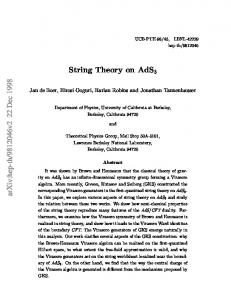
where the ± is needed to cover all regions of field space (φ, s) in the ± gravity patches in the (φ, s) plane as seen in Fig. 1. It is also possible to replace ss by −ss in Eq.(13) for another parametrization of the gauge choice as we will discuss below. Although the ± signs cancel out in the Lagrangian, it does not cancel out in the equations of motion, so solutions need to be continuous as φ or s vanish and change sign. The s-gauge in (13) corresponds to a pair of curves in the (φ, s) plane where points on the curves are parametrized by Φ according to (φs (Φ) , ss (Φ)) as shown in Fig. 1. ssHFL antigravity + region
gravity + region
increasing F
ΦsHFL inreasing F
gravity - region
antigravity - region
FIG. 1: Two branches of the curve in the parametric plot of the string gauge (φs (Φ) , ss (Φ)) in the ± gravity regions are shown. The origin corresponds to Φ = +∞ while the far left/right ends of the curve correspond to Φ = −∞. Each of the four wedge-shaped patches of field space is geodesically incomplete. The boundary of the gravity/antigravity regions, defined by |s| = |φ| , is shown with dashed lines. Geodesically complete solutions of the equations of motion cannot be constructed in the s-gauge with only the branches of the curve shown in Fig.1. Geodesic completeness requires additional branches in the antigravity regions.
If ss is replaced by −ss in (13) we get a new set of curves in the ± gravity regions that are similar to the pair of curves in Fig. 1, but mirror-reflected through the horizontal axis (s → −s). 8
Later we will discuss the possibility of including patches in which (φ2 − s2 ) is negative by simply interchanging cosh and sinh that modifies the gauge choice above leading to curves that look like 90o rotated in relation to those described above. These extend the domain of the string gauge into patches of antigravity (negative gravitational “constant”, as seen from (12)) which are required for geodesically complete cosmological spacetimes as discussed in a similar setting in [3]-[9]. The existence of such additional patches is not evident in the effective string action (2), but the study of particle geodesics shows that the spacetime described by (2) is geodesically incomplete, and this is a hint that invites a study of the complete space by including antigravity patches, as discussed below. With this choice of s-gauge in the gravity patch we see that the coefficients of the curvature R in (12) and (2) match each other, and furthermore the kinetic energy terms of (φs , ss ) in (12) precisely reproduce the kinetic energy term of the dilaton Φ in (2), with its unusual √ −2Φ s normalization, −G e2κ2 4 (∂Φ)2 . In order to have also Hµνλ match the expression in (3), it d
is necessary to determine the homogeneous function T (φ, s) such that in the string gauge (13) it reduces to a constant as a function of Φ, namely T (φs (Φ) , ss (Φ))=constant with either set of ± signs in (13). We find that before gauge fixing, and in the gravity patch (φ2 − s2 ) > 0, the homogeneous T (φ, s) of degree 4/ (d − 2) must be given by T (φ, s) =
�
d−2 4 (d − 1)
2 � d−2
√
d−1 2 1+d−2
(φ + s)
(φ − s)
√
d−1 2 1−d−2
,
(14)
or the same expression with s replaced by −s in Eq.(14) as well as Eq.(13). This T (φ, s) is normalized such that it reduces to the constant string tension in the gravity patches in the s-gauge given above (recall (4)) πT (φs (Φ) , ss (Φ)) = κ2d
2 �− d−2
=
1 . 2α′
(15)
As already mentioned, in antigravity patches where (φ2 − s2 ) < 0 we must exchange cosh and sinh in equation (13). We may then choose signs in (13) to ensure that the string tension T as defined in (14) behaves smoothly across the boundary between gravity and antigravity regions. Notice that the overall constant or sign in front of the tension is irrelevant at this point since only T −1 ∂λ T (which is insensitive to the sign of T ) appears in Hµνλ . It is notable that in the critical dimension d = 10 for superstrings or heterotic strings, we may choose signs so that the power of φ + s (or φ − s) appearing in the dynamical string tension (14) is unity, for both the gravity (or antigravity) patches. This means that, in a 9
suitable Weyl gauge, smooth cosmological transitions from gravity to antigravity, or vice versa, are associated with a smooth analytic sign change of the dynamical string tension T . Such transitions do in fact occur in generic homogeneous cosmologies [6], in a suitable Weyl gauge, termed γ-gauge, which will shortly be explained. We emphasize that the signs of (φ + s) and (φ − s) are Weyl gauge invariants, so their signs in every gauge are the same as those displayed in the geodesically complete γ-gauge solution displayed below. Finally, the potential energy that matches V (φs , ss ) =
d−26 e−2Φ , 3α′ 2κ2d
is also determined such
that before gauge fixing V (φ, s) is given by V (φ, s) =
� (d − 26) (d − 2) 2 φ − s2 T (φ, s) . 12 (d − 1)
This V (φ, s) is homogeneous of degree
2d d−2
(16)
as required in (10), it vanishes for d = 26 and is
negative for d < 26 in the gravity patch. It is expected that higher perturbative terms in α′ , non-perturbative, and string-string interaction effects will alter the effective low energy potential. Furthermore in supersymmetric or heterotic versions of string theory V is not the same as above (e.g. (d − 26) is replaced by (d − 10) in SUSY). In any case it is evident that the final phenomenologically significant result for V (φ, s) can always be rewritten in a Weyl 2d
covariant form as, V = φ d−2 f (s/φ) , for some Weyl invariant f (s/φ) as in our previous work. By determining the functions T (φ, s) and V (φ, s) as in (14,16), we have completely fixed the effective low energy string action as a Weyl invariant action in the gravity patch (φ2 − s2 ) ≥ 0 in the form given in Eqs.(12,6). A significant property of the new Weyl invariant effective action is that it becomes geodesically complete by including all field patches in the infinite (φ, s) plane in the sense discussed in our previous papers and later in this paper. To complete the definition of the geodesically complete string action in this sense we need to weigh carefully the possibilities of whether the smooth continuation of the functions T (φ, s) and V (φ, s) to all patches will change sign when crossing the transition lines |φ| = |s| in the (φ, s) plane which separate gravity/antigravity patches. This will be discussed below in the context of the string action with a dynamical tension T (φ, s) after a description of geodesic completeness across gravity/antigravity boundaries given below.
10
A.
Gauge choices for local scale symmetry and geodesic completeness
The Weyl invariant action (12) has no dimensionful constants of any kind. Besides the string gauge given in (13) where the gravitational constant (or the string tension) is introduced as the gauge fixed value of a combination of fields, the same action can be gauge fixed to other gauges that are useful for various physical applications especially in cosmology as discussed in [2]-[9]. Some of these gauges will be useful in string theory as well, so we review here some convenient gauge choices of the geodesically complete Weyl invariant action (12), and then describe the nature of geodesic completeness in each gauge. • s-gauge: This is the “string gauge” we used above in Eq.(13). A property of this gauge is that it satisfies |φ−s | = cd |φ+s |λd where cd , λd are some constants, and φ±s ≡ φs ±ss .
More precisely, as seen from (13), with the choice of cd =
�
κ2d (d − 2) 4 (d − 1)
�√
1 d−1−1
√ d−1+1 , λd = √ , d−1−1
(17)
φs (Φ) , ss (Φ) are parametrized in the ± gravity patches in terms of a single field Φ as in (13) so that the Weyl invariant action (12) is reduced to the gauge fixed action that matches the effective string action Sef f in (2). Other choices of (cd , λd ) would yield some similarly gauge fixed action, but a different one than (2). The expressions in (13) by themselves are insufficient to express the gauge choice in all regions of the (φ, s) plane. These equations must be supplemented by similar expressions that include more branches of the curve in Fig. 1. The additional branches correspond to curves obtained from Fig. 1 by a reflection through the horizontal axis generated by s → −s (new curve still in gravity), plus those obtained by a 90o rotations of the curves already mentioned, leading to additional branches in the antigravity patches. Later we will introduce a “flip symmetry” in Eq.(28) which relates to a symmetry that interchanges gravity and antigravity. To express the generic geodesically complete cosmological solution, given in Fig. 2 and Eqs.(20-25) below in the γ-gauge as a function of conformal time x0 , we need all of those additional branches in the string gauge basis (φs (Φ (x0 )) , ss (Φ (x0 ))). Accordingly, the geodesically complete form of Fig. 1 must include connections among all the branches of the curves described above, such that any given branch connects continuously to another branch 11
across the gravity/antigravity intersection by passing through the origin in Fig. 1 tangentially to one of the dashed lines while being perpendicular to the other. • E-gauge: This gauge is useful to rewrite the theory in the Einstein frame where the main physical intuition about gravitational phenomena is developed. Starting in the ± gravity patches, it is defined by gauge fixing (φ2 − s2 ) to a positive constant, (d−2) 8(d−1)
(φ2E − s2E ) =
1 . 2˜ κ2d
For the kinetic term of the remaining scalar (called σ) to be
normalized conventionally, − 21 (∂σ)2 , the fields (φ, s) are parametrized in terms of the field σ as follows q � � (d−2)˜ κd 1 cosh σ , φE (σ) = ± 4(d−1) (d−2) κ 4(d−1) q ˜d � � (d−2)˜ κd 4(d−1) 1 sE (σ) = (± or ∓) (d−2) κ˜d sinh 4(d−1) σ ,
(18)
� E The geometrical fields are also labeled with the letter E : gµν , bE µν . In this gauge the
E tension T (φE , sE ) obtained from (14) is not a constant and therefore Hµνλ as defined
in (6) has a non-trivial structure3 . The E-gauge in the gravity patches alone, as given in (18), is geodesically incomplete because one can find classical solutions of the fields in which the gauge invariant quantity (1 − s2 /φ2 ) changes sign as a function of time.
This happens when both (φE , sE ) are infinitely large (or σ →large) so that (1 − s2E /φ2E )
can vanish even though (φ2E − s2E ) is a constant all the way to the boundary of the gravity/antigravity patches. Hence the gravity patch by itself is incomplete. This is confirmed by noting that particle geodesics reach cosmological singularities in a finite amount of time. Furthermore, solutions of the field equations that extend to the gravity/antigravity boundary (see Fig. 2) show that when the gauge invariant E (1 − s2E (x) /φ2E (x)) → 0 the spacetime metric gµν (x) has also a curvature singularity
in the E-gauge. Hence the transition from gravity to antigravity patches occurs only at spacetime singularities in the Einstein frame. To obtain the gauge fixed expressions for (φ, s) in the antigravity patches in the E-gauge the cosh and sinh in (18) are interchanged; then the kinetic term of σ also changes sign. 3
A straightforward Weyl rescaling of (2) to the Einstein frame in which only Gµν is rescaled is also possible. But only the transformation of the metric produces a different expression for the transformed action. This E is because the untransformed Hµνλ or Bµν differ form our definitions of Hµνλ and bE µν by the extra terms E E E involving b[µν ∂λ] ln T . After writing bµν in terms of Bµν and expressing σ in terms of Φ (see below) we do recover the same results.
12
• c-gauge: This gauge is useful to relate the Weyl invariant theory to low energy degrees of freedom [14], and was used in the construction and analysis of the standard model coupled to gravity [1][8]. It is introduced by gauge fixing the field φ to a constant, φc (x) = c, and then sc (x) is the remaining dynamical scalar, while the � c other fields are labeled as gµν , bcµν . When sc is much smaller than the constant φc , which is true at energies much smaller than the Planck scale, the factor (φ2c − s2c (x))
is practically a constant from the perspective of low energy physics. This gauge is geodesically complete because (φ2c − s2c (x)) can change sign dynamically (as seen in c explicit solutions, including Fig. 2) when the spacetime gµν transits between gravity
and antigravity at curvature singularities. • γ-gauge: This gauge has been the most useful in simplifying equations and lead-
γ ing to analytic results. The determinant of the spacetime metric gµν is fixed to be � unimodular, det (g γ ) = −1, while the other fields are labeled with γ as φγ , sγ , bγµν . � For example for a cosmological spacetime of the form ds2γ = a2γ (τ ) −dτ 2 + ds2d−1
where τ is the conformal time, and ds2d−1 includes space curvature and anisotropy, the Weyl symmetry is used to gauge fix the scale factor to a constant for all conformal time, aγ (τ ) = 1. The γ-gauge is geodesically complete. It was used in cosmological
applications in [2]-[7] and led to the discovery of the geodesically complete nature of spacetime across big bang and big crunch singularities where the gravity-antigravity transition occurs [5][9]. • f (R) gravity gauge: If we choose (φ − s) to be a constant, φf (x) − sf (x) = c, then the kinetic term for the remaining field φ+ (x) ≡ φf (x) + sf (x) drops out of the action (12). Ignoring the H 2 term in (12), the field φ+ (x) becomes a purely algebraic field
that can be determined via the equations of motion (for any V ) to be a function of the �� curvature φ+ = φ+ R g f . Inserting this solution back into the action (12) reduces it to a function of only R. This is f (R) gravity, where the function f (R) is determined
by V (φ, s) (see also [13]). The transformations of fields from one fixed gauge to another is easily obtained by considering gauge invariants under the Weyl transformations. Some useful gauge invariants that
13
may be used for this purpose are d−2 d−2 √ � d−2 s √ � d−2 −g 2d φ, −g 2d s, |T (φ, s)|− 4 φ, |T (φ, s)|− 4 s, etc. , φ
(19)
To illustrate this, consider the example of the s-gauge versus the E-gauge. By comparing the gauge invariant,
ss (Φ) φs (Φ)
=
sE (σ) , φE (σ)
we obtain the relation between the dilaton Φ (x) in the
s-gauge (13) and the scalar field σ (x) in the E-gauge (18). This provides the local scale transformation ΩsE (x) that relates the s and E gauges according to Eq.(8), and using it we find � 4 E the relation between the remaining degrees of freedom, (Gµν , Bµν ) = (ΩsE )− d−2 gµν , bE µν . Thus, solutions of equations of motion in one gauge can be used to obtain solutions in all other gauges via the Weyl transformations among fixed gauges. Such field transformations are duality transformations: in each gauge the form of the action, the spacetime and the dynamics appear different, but the Weyl invariant physical information is identical. Indeed the stringy T-duality of the effective string action discussed in [16] is an automatic outcome of the Weyl invariant formalism discussed here. This is because the dualities based on inversion of scale factors in different directions [16] can be re-stated as a combination of general coordinate reparametrizations and local Weyl transformations, both of which are symmetries of our low energy string formalism in (12). In our setting here we can construct a richer set of dualities based on Weyl transformations between different gauge fixed versions of the same Weyl invariant effective low energy string theory (equivalently, dual backgrounds for string theory on the worldsheet)4 . Having shown that the low energy effective string theory (2) is just a gauge choice of the Weyl-lifted low energy string theory (12), we now are in a position to argue that by allowing the fields to take values in the full (φ, h) plane, including the antigravity regions shown in Fig. 1, we obtain a geodesically complete theory. To see this, we solve analytically the cosmological equations of motion that are predicted by (12) as shown in the next paragraph, and find that the dynamics requires that solutions that begin initially anywhere in the gravity patches (such as those shown in Fig. 1) evolve inevitably into the antigravity patches, thus requiring the inclusion of all patches. Then a geodesically complete field space includes 4
Weyl symmetry follows from 2T-physics in 4+2 dimensions as a requirement for its conformal shadow in 3+1 dimensions. Indeed, Weyl rescalings in 3+1 are simply local reparametrizations of the extra 1+1 dimensions as a function of the 3+1 dimensions [14]. In this connection see [15] where an even larger concept of dualities in phase space (beyond just position space), that follow from 2T-physics, is discussed.
14
all of the (φ, s) plane as well as an extension of the spacetime metric gµν (x) as a function of spacetime xµ to include the antigravity patches. In this complete field space geodesics (appropriately defined to be Weyl invariant as consistent solutions of the same theory [9]) are complete curves that do not artificially end at cosmological singularities [9]. Hence we have argued that the Weyl invariant low energy string theory (12) which includes all field patches is geodesically complete, at least for spacetimes of interest in cosmology. The behavior of the general solution in the vicinity of cosmological singularities is unique due to an attractor mechanism discovered in [5]. It can be argued that the generic solution is kinetic energy dominated so that the potential energy V is negligible. Taking also bµν = 0 for simplicity, but adding conformally invariant massless fields (treated as radiation ρr /a4 (x0 ) ), we display the solution obtained in [5] in four dimensions, d = 4, as follows. For our γ purposes here it is most simply described in the γ-gauge. The metric gµν is diagonal and
generically anisotropic near singularities and is parametrized as ! 3 X � � 2 2 e2i dxi ds2 = a2γ − dx0 + , a2γ = 1 (γ-gauge),
(20)
i=1
e21 = e2(α1 +
√
3α2 )
, e22 = e2(α1 −
√
3α2 )
, e23 = e−4α1 ,
(21)
where α1,2 (x0 ) are two dimensionless geometrical fields that parametrize the anisotropy γ such that e21 e22 e23 = 1, so the metric gµν is unimodular. The general generic solution for
α1 , α2 , φγ , sγ is [5] α1 α2 φ γ + sγ φ γ − sγ
x0 p1 , ln 4 = 0 0 2p l1 ρr (x − xc ) x0 p2 , ln 4 = 2p l2 ρr (x0 − x0c ) (p+p3 )/2p x0 2 0 0 = l3 ρr (x − xc ) 4 , l3 ρr (x0 − x0c ) −(p+p3 )/2p x0 2x0 . = 2 4 l l ρr (x0 − x0 ) 3
3
(22) (23) (24) (25)
c
Here x0 is conformal time as seen from the definition of the metric in (20). The constant parameters (l1 , l2 , l3 ) are constants of integration that have dimension of (length); the parameters (p1 , p2 , p3 ) are constants of integration that have dimension of (length)−2 , while p p ≡ p21 + p22 + p23 ; the constant ρr that represents the radiation density has dimension of √
(length)−4 ; finally x0c ≡ − κρ6pr is the time of the crunch while the bang is set at zero time. 15
sΓ Ix0 M
antigravity
ΦΓ Ix0 M bang
crunch
gravity gravity antigravity
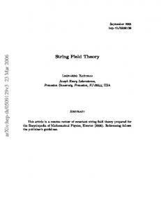
γ FIG. 2: Geodesically complete spacetime requires the antigravity loop. The solution for (φγ , sγ , gµν )
is continuous at the crunch x0 = x0c < 0 and the bang x0 = 0. The duration of the antigravity loop √ is x0c = κρ6pr . Geodesics in this spacetime go smoothly through both the crunch and the bang [9]. So information sails through singularities in this spacetime.
This solution is plotted parametrically in Fig. 2. The arrows on the curve show the evolution of the fields (φγ (x0 ) , sγ (x0 )) as conformal time x0 increases from negative values to positive values as the system goes through the crunch singularity at x0 = x0c and the bang singularity at x0 = 0. At the instants of crunch or bang the scale factor aE (x0 ) in the Einstein gauge, which in 2 2 d = 4 is given by [5], a2 = κ φ2 − s2 = κ ρr |x0 (x0 − x0 )| , vanishes, and the corresponding E
6
γ
γ
c
6
scalar curvature in the Einstein frame, R (gE ) , blows up. However in the γ-gauge, since
aγ = 1, the behavior is much milder since aγ is a constant, which is how we were able to obtain our geodesically complete analytic solutions in the γ-gauge. If the anisotropy coefficients p1,2 are non-zero, then the Weyl invariant Weyl curvature tensor, C µνλσ (g) , is singular in all gauges, including in the γ-gauge. However, this fact did not prevent us from obtaining [5] our geodesically complete solutions as given above explicitly, nor did it stop the geodesics in this geometry from sailing through the cosmological singularities in the presence of anisotropy [9], thus showing that information does go through singularities in our cosmological geometry in Eqs.(20-25). The underlying reason and technique for our ability to complete the geometry and geodesics across these singularities is the identification of a sufficient number of conserved quantities in our equations that allows us to match continuously all observables, finite or infinite, across the singularities [5][9]. The completion 16
of all geometrical features on both sides of singularities is evident since all observables, including those gauge invariants that blow up such as C µνλσ (g γ ) , are constructed from our solutions for α1 , α2 , φγ , sγ which are continuous through the singularities. The solution displayed in Fig. 2 is generic, exact, and includes all possible initial conditions (isotropic limit as well), hence there are no other solutions in our setting (12) under the conditions stated above (in particular, V = 0). However, since V cannot be neglected away from the singularities this solution is useful mainly to study the neighborhood of the singularities analytically, which is in fact our focus, and of course precisely where string theory would play a role. So this geodesically complete geometry is of great interest to string theory. When V 6= 0, the complete set of solutions are known analytically for certain potentials V when anisotropy is neglected [6]. The analytic expressions and their plots [6] are sufficient to infer the solution for more general potentials V. Combining the attractor behavior near the singularities which is induced by anisotropy (Fig. 2) together with the known behavior away from singularities when anisotropy is negligible, the general generic behavior is pretty well understood as follows: When V is included, the generic solution is such that the trajectory shown in Fig. 2 continues to move to large values of φγ in the gravity region, while sγ oscillates at much smaller amplitudes (see illustrations in [3],[4],[7],[8]). So, when the trajectory in the (φγ , sγ ) plane shown in Fig. 2 is continued to larger times beyond the singularities, the curve turns around at large values of φγ and comes back for another crunch at the origin of the (φγ , sγ ) plane, passes through another antigravity loop and after another bang continues to the opposite gravity region, doing this again and again an infinite number of times as conformal time keeps progressing from minus infinity to plus infinity. The Weyl invariant system in Eq.(12), coupled to ordinary matter (here symbolized by the radiation parameter ρr ), is then like a perpetual motion machine, which absorbs energy from the gravitational field and creates additional entropy during antigravity in each cycle [8], thus yielding generically a cyclic universe, whose global scale in the Einstein frame, aE (x0 ) , grows progressively in each cycle due to entropy production, without having an initial cycle in the multicycles in the far past or an end of multicycles in the far future [8]. There are of course quantum corrections to this picture. Unfortunately, these will remain obscure until quantum gravity is under better control. In the interim, some new directions of research emerge from interesting new questions that arise about the quantum physics during 17
the antigravity period and close to singularities. There are signals of instability because the kinetic energy term for the gravitons is negative during antigravity. It seems gravitons would be emitted copiously to transit to a lower energy state in response to this instability. However, to maintain the energy constraints due to general coordinate invariance ordinary matter must also be emitted simultaneously. This is good for entropy production from one cycle to the next as discussed in [8]. Note that a measure of the amount of time spent in the antigravity regime is |x0c | =
√
6p κρr
as seen from our analytic solution (20-25) and Fig. 2 above.
If radiation ρr (any relativistic matter) increases by entropy production during antigravity as mentioned above, then the antigravity period |x0c | gets shorter. This is a signal that there seems to exist a built-in dynamical recovery process to get from antigravity back to gravity. We hope that the string version of our formulation below can shed light on the microscopic stringy details of this mechanism. The low energy theory has produced a wealth of signals for previously unknown interesting phenomena. The general generic features we have noted in [1]-[9] are likely to survive in the context of quantum gravity when we understand it better. To counter comments such as those in [17][18], as we did in [9], it may be worth remembering that in string theory singularities tend to get smoother or resolved, so we should expect less singular behavior as compared to the low energy theory as stringy features are taken into account. It is not advisable to try to include in our analysis stringy features in the form of higher derivative corrections in the effective action. This is because those corrections to the action are computed under the assumption of low energy away from singularities, so they are the wrong tool to analyze phenomena near singularities. Rather, we need to tackle string theory directly and ask again in that context the types of questions we have been able to analyze and partially resolve in the low energy theory. However, the starting point of string theory does not seem to be well suited for our type of analysis since it begins with a dimensionful constant, namely the string tension. For this reason we seek a more general starting point, one in which the string tension is replaced by a background field just like the gravitational constant which was replaced by a field in the low energy theory. The construction of such a string theory is the topic of the next section.
18
III.
WEYL INVARIANCE AND DYNAMICAL TENSION IN STRING THEORY
The goal in this section is to develop a Weyl invariant formalism for strings propagating in backgrounds, so that the string tension (2πα′ )−1 - equivalently the gravitational constant - emerges from the gauge fixing of a background field in a new string theory that has a local scaling gauge symmetry acting on target space fields. Taking the clues developed in the previous section we propose the following string action with a dynamical string tension and target-space Weyl symmetry. We simply insert in (1) our expressions for the Weyl covariant substitutes for 2α′ and Φ in terms of (φ, s) as given in Eq.(14) and Eq.(13). The result is � √ Z 1 ab ab µ ν − T (φ (X) , s (X)) −hh g (X) + ε b (X) ∂ X ∂ X µν µν a b 2 �2 � S = d2 σ √ √ � φ(X)+s(X) d−1 1 (2) + 16π −hR (h) ln φ(X)−s(X) + O T
(26)
where X µ (τ, σ) is the string coordinate. If we insert the s-gauge expressions for � s φs , ss , gµν , bsµν given in Eq.(13) for the ± gravity patches, this action reduces to the stan-
dard string action in Eq.(1). For this more general action to be consistent with the worldsheet conformal symmetry up to order (1/T ) , the target space Weyl covariant background fields (φ, s, gµν , bµν ) must be classical solutions of the equations of motion that are derived from the target space Weyl invariant effective action (12). The relevant solutions were described in the previous section. The appearance of the logarithm in the action (26) might be a cause for concern, since √ the Lagrangian density appears non-analytic. However, since the Euler density −hR(2) is a total derivative, one can integrate by parts, so that the resulting Lagrangian density, involving only first order derivatives, has no branch cuts and is single-valued on field space. This string action contains no dimensionful constants. It is Weyl invariant when the target-space background fields (φ, s, gµν , bµν ) are rescaled locally according to the rules in Eq.(8). This is easily seen by noting that the combinations of fields s gˆµν ≡ T (φ, s) gµν , ˆbµν ≡ T (φ, s) bµν , φ
(27)
that appear in the basic string action (26) are Weyl invariant. We will see below that they also obey an additional symmetry which we call flip symmetry, that allows us to extend T (φ, s) , from the ± gravity patches where it was initially defined in (14), to the geodesically complete entire (φ, s) plane. 19
Therefore it is possible to Weyl gauge fix the action in various ways (e.g. s, E, c, γ, f gauges of the previous section) to investigate the physics of string theory in the corresponding spacetimes that look like different backgrounds from one another. Any results obtained in one Weyl gauge are easily transformed to another gauge, just like duality transformations (which are now realized as Weyl transformations as explained at the end of the last section). This expression for the string action is so far uniquely determined in the gravity patches (φ2 − s2 ) ≥ 0 where the dynamical tension T (φ, s) is positive. In this sense, with Eq.(26), we have already achieved a non-trivial stage for the target-space Weyl invariant definition of string theory. The remaining questions involve the sign of the dynamical tension T (φ, s) in the antigravity patches so that the theory is sensible according to sacred principles, such as unitarity, since a negative sign of T in (26) may imply negative norm states. We will show below that unitarity is not a problem, but there are physics questions to consider. We emphasize that the issue is subtle because the antigravity patches occur only for a finite amount of time |x0c | in our cosmological solutions and during that period those space-time patches are separated by cosmological singularities from our own observable gravity patch, as seen in Fig. 2. In considering the sign of T (φ, s) in the antigravity patches, there is an additional clue in the low energy Weyl invariant action (12) to take into account. We observe that all the kinetic terms of the action in (12) flip sign if φ and s are interchanged with each other. Independently, if the metric gµν flips signature, gµν → −gµν , then noting R (−g) = −R (g) , and that ∂φ · ∂φ, ∂s · ∂s, H 2 all contain an odd power of g µν , while (− det g) is invariant
for even d, we see that all kinetic terms in (12) flip sign under the signature flip. Therefore, under the simultaneous flip of signature and interchange of (φ, s) flip symmetry: (φ ↔ s) and gµν → −gµν ,
(28)
all kinetic terms of the low energy action (12) are invariant for even d. It is possible to include a flip of sign of bµν → −bµν , as an additional part of the flip transformations in (28), since the flip of bµν is also a symmetry all by itself in the low energy action. Observe also that Hµνλ as given in (6) is automatically flip symmetric for the T given in (14). The remaining term in (12) is the potential energy V (φ, s) , whose properties under the flip transformation is unclear at this stage but should be determined by the underlying string theory. Since the low energy action has a flip symmetry (at least in its kinetic terms) we ex20
pect that the underlying string theory action (26), which should be compatible with all properties of (12), should be symmetric under the flip transformation of all its background fields. Requiring this symmetry uniquely determines the properties of T (φ, s) in all gravity/antigravity patches because the combinations T (φ, s) gµν and T (φ, s) bµν that appear in (26) must now be required to be flip symmetric. This determines uniquely that T must be antisymmetric under the interchange of (φ, s) T (φ, s) = −T (s, φ) .
(29)
Therefore the continuation of the expression T (φ, s) in (14) from the original gravity patch to all other gravity/antigravity patches must obey this requirement. This can be done by writing Tstring (φ, s) = (φ2 − s2 ) | Tφ2(φ,s) | thus extending the T (φ, s) in (14) to the entire (φ, s) −s2 plane. In what follows we will assume that this has been done, but to avoid clutter, we will continue to use the symbol T (φ, s) to mean the properly continued Tstring (φ, s) . This completes the definition of the Weyl symmetric string action in (26).
A.
String in Geodesically Complete Cosmological Background
We will investigate the proposed action (26) for the geodesically complete cosmological background in Eqs.(20-25) that includes both gravity and antigravity patches as shown in Fig. 2. This background is consistent with worldsheet conformal invariance since it is the generic solution of the equations of motion of the effective action (12). This background, which is an exact solution when V = 0, and otherwise is the correct approximation near the singularity even when V 6= 0, is suitable for our purpose of analyzing what happens near the gravity/antigravity transitions. The worldsheet conformal symmetry has been insured for any dimension d (to lowest order in α′ ). Since the background in Eqs.(20-25) was computed in four dimensions, we will specialize to d = 4 without losing the (perturbatively valid) worldsheet conformal symmetry. We first compute the dynamical string tension (14) for d = 4 for this background using Eqs.(14,24,25) T4
√3 � � φ + s 1 1 γ γ φ2γ − s2γ X0 = = ρr X 0 (X 0 − x0c ) 6 φ γ − sγ 3 21
p3 /p ! 1 X0 4 2 l3 ρr (X 0 − x0c )
√
3
(30)
Here X 0 (τ, σ) is the string coordinate which is the conformal time in the given background geometry. This T4 (X 0 ) is flip antisymmetric as discussed in the previous section. γ The metric gµν was given in Eq.(20). But we emphasize that only the Weyl invariant γ combination gˆµν = T (φγ , sγ ) gµν enters in our action, with
� dˆ s2 = gˆµν dxµ dxν = T x0
0 2
√ 2(α1 + 3α2 )
1 2
− (dx ) + e (dx ) . √ 2 2 +e2(α1 − 3α2 ) (dx2 ) + e−4α1 (dx3 )
(31)
Explicitly, this purely time (string X 0 ) dependent cosmological background for a string theory with dynamical tension is √
gˆ00 (X) = gˆ11 (X) = gˆ22 (X) = gˆ33 (X) =
√ 3p3 3p3 X0 p 4 − p , (ρr l3 ) X 0 −x0c √ √ √ √ p1 3p2 3p3 p1 + p + p 3p2 3p3 ρr X 0 (X 0 −x0c ) X 0 p 4 − p 4 − p 4 − p √ (ρ l ) (ρ l ) (ρ l ) , r r r 0 0 1 2 3 3 X −xc 2 3 √ √ √ √ p1 3p2 3p3 p1 3p2 3p3 − p + p 0 −x0 ) ρr X 0 (X X0 p 4 − p 4 + p 4 − p c √ (ρ l ) (ρ l ) (ρ l ) , r r r 0 0 1 2 3 X −xc 2 33 √ √ 2p1 3p3 2p1 + p − 3p3 ρr X 0 (X 0 −x0c ) X 0 p 4 p 4 − p √ (ρ l ) (ρ l ) . r r 0 0 1 3 X −x 2 33
0 0 −x0 ) c √ − ρr X 2(X 33
(32)
c
where the parameters (p1 , p2, p3 , p, l1 , l2 , l3 , ρ, x0c ) are defined after Eq.(25).
Note that in the low energy effective theory the original metric gµν in (12) does not change sign as the trajectory in Fig. 2 transits from a gravity region to an antigravity region at cosmological singularities. Instead, the dynamical gravitational “constant” (φ2 − s2 ) , that multiplies the curvature in the low energy action (12), changes sign at those singularities. However, in view of the flip symmetry (28) of the geodesically complete low energy theory (12), the sign flip of the factor (φ2 − s2 ) can also be viewed equivalently as being a signature flip of the effective metric gˆµν defined above, since R (−ˆ g ) = −R (ˆ g ). Indeed the effective
metric gˆµν (X 0 ) in (32) changes overall signature precisely at the cosmological singularities. The period of antigravity (or opposite signature of gˆµν ) and its temporary duration, |x0c | = √
6p , κρr
is determined by the physical parameters of the background above.
Just as we could study particle geodesics in this background in [9], we can also study string geodesics in this geodesically complete geometry by solving the equations for X µ (τ, σ) that follow from our action (26). This topic is partially explored in the next section.
22
B.
Unitarity with a Temporary Flip of the Dynamical String Tension
In this section we study a formalism for solving generally the classical solutions and the quantization of the string theory described by our action (26), and its specialization to a cosmological background given in Eq.(32). To simplify this investigation we will drop the quantum correction terms for worldsheet conformal symmetry in (26) as well as the bµν background field since these are not the crucial terms for our questions involving the temporary sign flip of the dynamical string tension. Hence we will simply concentrate on the purely classical string action which is modified only by the dynamical string tension Z √ 1 Scl = − d2 σ −hhab gˆµν (X) ∂a X µ ∂b X ν , (33) 2 where the tension is absorbed into the definition of gˆµν = T gµν , allowing gˆµν to have a temporary signature flip. We are interested in obtaining the solutions for strings in such backgrounds, and quantizing them to answer the questions on unitarity and begin to interpret the physics when there is a signature or tension flip. Since such questions are more general than the specific background in (32), we will consider a more general gˆµν . Much of the necessary canonical formalism was developed in Ref. [19]. It is useful to introduce the momentum density defined by Pµa ≡ ∂Scl /∂ (∂a X µ ) , √ hba (34) Pµa = − −hhab gˆµν ∂b X ν , ⇒ ∂b X ν = − √ gˆνµ Pµa , −h where the canonical conjugate to X µ corresponds to the momentum density Pµτ , i.e. when a = τ. The classical string equations of motion and constraints that follow from this action are δX µ : 0 = ∂a
√
� −hhab gˆµν ∂b X ν −
√
−hhab ∂a X λ ∂b X ρ ∂X µ 2
(ˆ gλρ )
δhab : 0 = gˆµν Pµa Pνb − 21 hαb hcd gˆµν Pµc Pνd .
(35)
To make progress we consider the worldsheet gauge hτ σ = 0 in which hab is diagonal. There is remaining worldsheet gauge symmetry to choose also the gauge X 0 = τ , which we will do √ later. Although a diagonal hab contains two functions, the combination −hhab contains only one function since its determinant is −1. Hence we parametrize hab as follows � � √ −h 0 ab . −hh = 0 1/h
(36)
and insert it in all the equations listed in (35). In what follows we will assume that the metric is diagonal as is the case in (32) � gˆµν = T × diag −1, e21 , e22 , e23 , · · · . 23
(37)
Then, Pµτ = hˆ gµν ∂τ X ν , Pµσ = −h−1 gˆµν ∂σ X ν
µ = i : 0 = ∂τ (−hˆ gii ∂τ X i ) + ∂σ (h−1 gˆii ∂σ X i ) , no sum on i 0 −1 0 ∂τ (−hˆ g00 ∂τ X ) + ∂σ (h gˆ00 ∂σ X ) µ=0: 0= � 1 λ ρ −1 λ ρ − 2 −h∂τ X ∂τ X + h ∂σ X ∂σ X ∂X 0 gˆλρ
(38)
0 = (P τ ± hP σ )2 or 0 = (h∂τ X ν ± ∂σ X ν )2 ,
The last constraint equations are solved as s gµν ∂σ X µ ∂σ X ν h = ε (X) , and gµν ∂τ X µ ∂σ X ν = 0, −gµν ∂τ X µ ∂τ X ν
(39)
Note that in these expressions we wrote gµν rather than gˆµν = T gµν because the tension factor of T (X) drops out. Here ε (X) is a sign function that emerges from taking the square root. Assuming hab has a fixed signature we must take ε (X) = 1 so that the signature of the metric in (36) remains fixed forever5 . 5
We make some remarks here on the possibility that the worldsheet may also be allowed to flip signature. Although we will not pursue this to the end in this paper, it could be important to keep it in mind. The general solution of the hab equation in (35) is expressed in several forms hab (X) = gˆµν (X) Pµa Pνb × ω −1 (X) , or hab (X) = gˆµν (X) ∂a X µ ∂b X ν × ω (X) .
(40)
The undetermined conformal factor ω (X) of the worldsheet metric in (40) is immaterial except for its √ sign because its absolute value always cancels in the worldsheet-Weyl invariant combination −hhab that appears in all equations. However, in view of the fact that the tension factor T in the action (33) can flip sign temporarily, we may entertain the possibility that the hitherto undetermined conformal factor ω (X) in (40) could also flip sign, thus inducing hab to flip or not to flip signature, perhaps simultaneously √ with T. Since only the combination T (X) −hhab gµν appears everywhere, the sign flip of T could be associated with gˆµν as already mentioned above, but it is also possible that in the solution of the theory as in (40) the flipping signature of gˆµν could be canceled by a flipping sign of the factor ω (X) . Considering such solutions of the theory amounts to associating the sign of T (X) with hab to combine them into an ˆ ab ≡ sign(T )hab that flips signature at the gravity/antigravity boundaries, while leaving the signature h of gµν unchanged. But to be able to admit such solutions, the string theory in Eq.(33) needs to be defined from the outset such that its worldsheet is permitted to have such properties. The signature flip of the effective ˆ hab amounts to the interchange of the role of τ, σ as timelike/spacelike coordinates on the worldsheet as soon as the string crosses the gravity/antigravity boundary. It is worth emphasizing that this should not create any ghost problems since the worldsheet still has only one time coordinate before or after the flip. If the string theory is defined to include such properties, then the quantization of the theory and the computation of amplitudes via the string path integral would need to admit the possibility of such worldsheets. Since this possibility has not, as far as we know, been considered before, we shall not pursue it further here.
24
Now, if we choose also the timelike gauge, X 0 = τ, we obtain the following form for the Hamiltonian density H (τ, σ) , which is the negative of the canonical conjugate to X 0 as given in Eq.(38), X 0 = τ ⇒ H (τ, σ) = −P0τ = h (τ, σ) T (τ ) ,
(41)
where we insert the solution for h in Eq.(39) to obtain the Hamiltonian density (with ε(X) set to 1) e2j (τ ) (∂σ X j )
H (τ, σ) = T (τ )
2
1 − e2j (τ ) (∂τ X j )2
!1/2
,
(42)
Here T (X 0 ) and e2i (X 0 ) are backgrounds, such as those in our suggested cosmological background in (32), evaluated at X 0 = τ . This Hamiltonian may also be expressed in terms of the canonical conjugate to X i , which is Piτ , instead of the velocity ∂τ X i . Using Piτ = hˆ gii ∂τ X i = T ×
e2j (∂σ X j )
2
1 − e2j (∂τ X j )2
!1/2
e2i ∂τ X i ,
the Hamiltonian density in terms of canonical conjugates is obtained as � � � 1/2 � T 2 (τ ) 2 j 2 −2 τ 2 e (τ ) ∂σ X . H (τ, σ) = T (τ ) ej (τ ) Pj + π2 j
while the velocity is also given in terms of canonical variables � � �−1/2 T (τ ) Piτ (τ, σ) Pτ � τ 2 2 2 j 2 ∂τ X i (τ, σ) = 2 (τ ) P + T (τ ) e (τ ) ∂ X = i2 e−2 . σ j j j ei (τ ) H (τ, σ) ei
(43)
(44)
(45)
Note that in a time dependent curved cosmological background there is no translation
symmetry in the time coordinate X 0 . Therefore we do not expect that the time translation generator P0τ would be conserved in the gauge X 0 = τ. Hence the Hamiltonian density or the total energy of the system which is given by the Hamiltonian H, Z H (τ ) = dσH (τ, σ) ,
(46)
will generally be a function of time τ in any cosmological background. Having dealt with the gauge fixed X 0 and its conjugate Hamiltonian, the remaining independent dynamical degrees of freedom X i (τ, σ) satisfy the following equations of motion and constraints 0 = −∂τ
He2i ∂τ X i
�
+ ∂σ
�
� e2i i ∂σ X , no sum on i H
0 = ∂σ X j Pjτ or 0 = e2j ∂τ X j ∂σ X j , summed over j 25
(47) (48)
The meaning of the constraint is the imposition of the σ-reparametrization gauge symmetry on physical states. The quantization of this system is now evident. The equal time quantum rules are � i � X (τ, σ) , Pjτ (τ, σ ′ ) = iδ (σ − σ ′ ) .
(49)
On the Hilbert space created by these canonical operators we must impose the physical state constraints which must be normal ordered at a fixed time τ � : ∂σ X i (τ, σ) Piτ (τ, σ) : |physi = 0.
(50)
This Hilbert space is clearly unitary, since we have shown that a unitary gauge exists in which only space-like canonical degrees of freedom are involved in the quantization of our system. Space-like degrees of freedom can never create negative norm states and the evolution of the system is generated by a Hermitian Hamiltonian. So, there are no issues with unitarity.
IV.
OUTLOOK
In this section we address some open problems and point out some tools and new directions to make further progress. We argued that there are no problems with unitarity. However, there is the unfamiliar feature, that the energy carried by any string configuration as predicted by Eq.(46) will become negative once the string (along with the rest of the universe) enters the antigravity patch. Taking our theory as a cosmological model, the negative energy is supposed to happen in between two cycles in an infinitely cyclic universe, so the question relates in particular to what happens just before our current big bang. This is precisely where we hope string theory could shed some light on quantum gravity. Is the negative energy during the antigravity period a problem like an instability, or just a new physics feature to investigate? How can we tell from our perspective as observers in the gravity patches separated from antigravity by cosmological singularities? One way to investigate this is to consider the analog of a scattering process in which we imagine a string probe that travels to the antigravity patch and returns to the gravity patch as an altered string that brings information from the antigravity region. Based on a set of solutions of this 26
nature, we have already verified that the behavior of string solutions as they pass through the crunch/bang singularities is regular and is physically sensible. This analysis will appear in a forthcoming paper. From the classical and quantum discussion above it is clear that the single string system represented by the Weyl invariant action (26), with the cosmological configuration (32) in mind, could not be unstable during antigravity. This is because when the energy is negative, it is negative for all classical and all quantum configurations of the single string during the entire antigravity period for the whole universe. There are no positive energy states of the single string during antigravity. Based on an adiabatic approximation of energy conservation, it is not possible to make a transition to a lower energy state because it is not possible to conserve energy adiabatically with only negative energy states. Hence there can be no transitions among the states of a single string that would indicate an instability in the system described by (26). What about a multi-string system that includes string-string interactions? A hint is provided by the flip symmetry of the low energy action. We have seen already that all the kinetic terms flip sign when either gµν flips signature or when (φ, s) are interchanged. This transformation can be used to infer the properties of the theory in the antigravity regime. If all terms of the effective action flip sign under the (φ, s) interchange, then we deduce that all equations of motion, and hence all physics, is the same during antigravity as compared to gravity, and therefore nothing strange should be expected during antigravity. If the potential V (φ, s) does not flip sign or has no definite flip symmetry, then after multiplying the overall action by an overall minus sign, the system would behave as if the potential is effectively time dependent when one compares the antigravity/gravity periods. Like in any time-dependent system, this system would undergo transitions. However this does not imply that any sacred principles of physics would be violated. Our considerations based on the low energy action and the flip symmetry of the kinetic terms are reassuring that the physics is still familiar, but we need better tools to understand the stringy details. For a more powerful tool to investigate string-string interactions we may turn to string field theory (SFT). This relates to our new action (26) since the corresponding SFT is constructed by using a BRST operator derived from the stress tensor for the Weyl invariant action (26). Therefore SFT provides a conceptual framework in which the relevant issues may be considered in a complete formalism that includes all the interactions. Although it is 27
hard to compute in SFT, recent improvements of its formulation [21] with a new Moyal-type star product that can be used for any curved space, makes it possible to use this as a tool for more progress to answer our questions in quantum gravity. For our purpose here the general structure of the open string field theory action [20] is already a guide, as follows. In the so called “Siegel gauge” the BRST operator boils down to the kinetic operator given by the Virasoro operator L0 , while the basic interaction is cubic as in Chern-Simons theory. After some manipulations, the open string field theory action can be gauge fixed to the following form of non-commutative field theory � 1 S = T r AL0 A + 2 R where L0 = dσ [Stress Tensor] , is the zeroth
� g A⋆A⋆A . 3
(51)
Virasoro operator. In the new formalism � τ [21] the string field A is a function of half of the string phase space A X+µ (σ) , P−µ (σ) , the trace T r is integration in the half phase space, while the star product ⋆ is the new
background independent Moyal star product (which represents string joining/splitting) in this half phase space6 . The point here is that L0 , as a function of the stress tensor of our � theory in (26) written in terms of canonical variables X µ (σ) , Pµτ (σ) , is the only part of SFT that contains the new information about the flipping dynamical tension T (X 0 (σ)) as a function of X 0 (σ) . Hence, this formalism is an arena that can be used to further investigate our questions including string-string interactions both perturbatively in the coupling g, and non-perturbatively including the search for the ground state as in any interacting field theory in the presence of interactions. In this context a first impression is that, cosmologically the negative energies will occur not only for single strings but for all strings in the universe at the same time, and hence there should be no instabilities, although there should be new physical features. It would be very useful to construct examples of worldsheet-conformally-exact string models whose string tension is Weyl-lifted to a background field as in Eq.(26). This would greatly improve the α′ expansion of Eq.(1) or the corresponding 1/T expansion in (26), to include all orders, and would also be essential in practice for the SFT approach discussed 6
The string phase space is X µ (σ) , Pµτ (σ) as defined above, and taken at fixed τ (no gauge choice for X 0 ). � µ τ Half of the string phase space is X+ (σ) , P−µ (σ) where the ± indicate parts of those string degrees of freedom that are symmetric and antisymmetric relative to the midpoint of the open string at σ = π/2 [21].
28
above. A starting point to pursue this idea could be the (gauged) Wess-Zumino-Witten models like those discussed in [22]-[24]. Ideally we would like to find a conformally exact cosmological string background whose behavior near the cosmological singularities matches the behavior explicitly computed in Eqs.(22-25) and Fig. 2, and whose effective metric near the cosmological singularities matches the form of Eq.(32) after including the dynamical tension. Pursuing duality concepts is bound to be helpful to clarify the questions mentioned above and to generalize our Weyl invariance approach to other corners of M-theory. We mentioned earlier the connection of our target space Weyl symmetry to dualities within the bosonic string theory in connection to scale inversions [16] and the more general cases involving transformations among the (s, E, c, γ, f )-type gauge choices (see also footnote (4)). There is more to consider on the duality path by pursuing the flip symmetry (28) further. A version of our flip symmetry was considered in [25][26] for a variety of supersymmetric and heterotic strings in the context of low energy string theory, but without our Weyl lifting ideas. We emphasize that without Weyl lifting such a symmetry is not really realizable in the standard formulation of string theory because, as stated in [25][26], it involves the sign flip of the effective string coupling eΦ to −eΦ . This cannot be achieved by any reasonable transformation of the dilaton Φ as a field that takes values only on the real line. However, with our Weyl lifting, there is also a factor related to the dynamical tension T that multiplies eΦ instead of the constant tension. It is the extra factor, not Φ, that transforms under our flip symmetry, and this is realized in our case by the interchange of (φ, s). We may consider the work in [25][26] as a possible guide toward the generalization of our Weyl lifted string theory (26) to a variety of dual corners of M-theory, including supersymmetric and heterotic versions, and to pursue duality concepts. The tools and ideas mentioned above offer concrete approaches to further exploration of string theory with target-space Weyl invariance and a dynamical string tension. We acknowledge conversations with Ed Witten on this topic. This research was partially supported by the U.S. Department of Energy under grant number DE-FG03-84ER40168 (IB) and under grant number DE-FG02-91ER40671 (PJS). Research at Perimeter Institute is supported by the Government of Canada through Industry Canada and by the Province
29
of Ontario through the Ministry of Research and Innovation.
[1] I. Bars, P.J. Steinhardt, N. Turok, “Local conformal symmetry in physics and cosmology,” Phys. Rev. D89 (2014) 043515 [arXiv:1307.1848]. [2] I. Bars and S-H. Chen, “The Big Bang and Inflation United by an Analytic Solution ”, Pays. Rev. D 83 043522 (2011) [arXiv:1004.0752]. [3] I. Bars, S-H. Chen and N. Turok, “Geodesically Complete Analytic Solutions for a Cyclic Universe”, Phys. Rev. D84 083513 (2011) [arXiv:1105.3606]. [4] I. Bars, “Geodesically Complete Universe”, arXiv:1109.5872, in the online Proceedings of the DPF- 2011 Conference, Providence, RI, August 8-13, 2011, http://www.slac.stanford.edu/econf/C110809/. [5] I. Bars, S.-H. Chen, P. J. Steinhardt and N. Turok, “Antigravity and the Big Crunch/Big Bang Transition”, Phys. Lett. B715 (2012) 278-281 [arXiv:1112.2470]. [6] I. Bars, S.-H. Chen, P. J. Steinhardt and N. Turok, “Complete Set of Homogeneous Isotropic Analytic Solutions in Scalar-Tensor Cosmology with Radiation and Curvature”, Phys. Rev. D86 (2012) 083542 [ arXiv:1207.1940]. [7] I. Bars, “Traversing Cosmological Singularities, Complete Journeys Through Spacetime Including Antigravity”, arXiv:1209.1068, in Beyond the Big Bang, Competing Scenarios for an Eternal Universe, Ed. Rudy Vaas, Springer [2013], ISBN 978-3-540-71422-4. [8] I. Bars, P.J. Steinhardt, N. Turok, “Cyclic Cosmology, Conformal Symmetry and the Metastability of the Higgs,” Phys. Lett. B726 (2013) 50 [arXiv:1307.8106]. [9] I. Bars, P.J. Steinhardt, N. Turok, “Sailing Through the Big Crunch-Big Bang Transition,” Phys. Rev. D89 (2014) 061302 [arXiv:1312.0739]. [10] M. Green, J. Schwarz and E. Witten, Superstring Theory, Vol.1, Cambridge Univ. Press 1987. [11] R. C. Myers, Phys. Lett. B 199, 371 (1987). [12] I. Bars, “Constraints on Interacting Scalars in 2T Field Theory and No Scale Models in 1T Field Theory”, Phys. Rev. D82 (2010) 125025 [arXiv:1008.1540]. [13] K. Bamba, S. Nojiri, S. Odintsov, D. S´ aez-G´ omez “Possible antigravity regions in F(R) theory?” Phys. Lett. B730 (2014) 136-140 [arXiv:1401.1328]. [14] I. Bars, “Gravity in 2T-Physics”, Phys. Rev. D77 (2008) 125027 [arXiv:0804.1585]; I. Bars,
30
S. H. Chen “Geometry and Symmetry Structures in 2T Gravity”, Phys. Rev. D79 (2009) 085021 [arXiv:0811.2510v2]. [15] I. Araya and I. Bars, “Generalized Dualities in 1T-Physics as Holographic Predictions from 2T-Physics,” Phys. Rev. D89 (2014) 066011 [arXiv:1311.4205]. [16] M. Gasperini and G. Veneziano “The Pre - Big Bang Scenario in String Cosmology,” Phys. Rept. 373 (2003) 1 [hep-th/0207130] [17] J. Carrasco, W. Chemissany, R. Kallosh, “Journeys Through Antigravity?,” JHEP 1401 (2014) 130 [arXiv:1311.3671]. [18] A. Linde, “Inflationary Cosmology after Planck 2013,” arXiv:1402.0526. [19] N. Turok, M. Perry and P. J. Steinhardt, Phys. Rev. D 70, 106004 (2004) [Erratum-ibid. D 71, 029901 (2005)] [hep-th/0408083]. [20] E. Witten, Nucl. Phys. B268 (1986) 253. [21] I. Bars and D. Rychkov, “String Field Theory with Background Independent Moyal-Star Product”, in preparation. [22] I. Bars and K. Sfetsos, Mod. Phys. Lett. A7 (1992) 1091; Phys. Rev. D46 (1992) 4495; Phys. Lett. B301 (1993) 183; Phys. Rev. D 48 (1993) 844. [23] C. Nappi and E. Witten, Phys.Rev.Lett. 71 (1993) 3751. [24] A. Tseytlin and K. Sfetsos, Nucl.Phys. B415 (1994) 116; Phys. Rev. D49 (1994) 2933; Nucl. Phys. B427 (1994) 245. [25] M. Duff and J. Kalkkinen, “Signature Reversal Invariance,” Nucl. Phys. B758 (2006) 161 [hep-th/0605273] [26] M. Duff and J. Kalkkinen, “Metric and Coupling Reversal in String Theory,” Nucl. Phys. B760 (2007) 64 [hep-th/0605274].
31