Dynamical symmetry breaking of lambda and vee-type three-level

Dynamical symmetry breaking of lambda and vee-type three-level systems on quantization of the field modes

arXiv:0802.0368v1 [quant-ph] 4 Feb 2008

Mihir Ranjan Nath1 and Surajit Sen2 Department of Physics Guru Charan College Silchar 788004, India Asoke Kumar Sen3 Department of Physics Assam University Silchar 788011, India Gautam Gangopadhyay4 S N Bose National Centre for Basic Sciences JD Block, Sector III Salt Lake City, Kolkata 700098, India

Abstract We develop a scheme to construct the Hamiltonians of the lambda, vee and cascade type of three-level configurations using the generators of SU (3) group. It turns out that this approach provides a well defined selection rule to give different Hamitonians for each configurations. The lambda and vee type configurations are exactly solved with different initial conditions while taking the two-mode classical and quantized fields . For the classical field, it is shown that the Rabi oscillation of the lambda model is similar to that of the vee model and the dynamics of the vee model can be recovered from lambda model and vice versa simply by inversion. We then proceed to solve the quantized version of both models introducing a novel Euler matrix formalism. It is shown that this dynamical symmetry exhibited in the Rabi oscillation of two configurations for the semiclassical models is completely destroyed on quantization of the field modes. The symmetry can be restored within the quantized models when the field modes are both in the coherent states with large average photon number which is depicted through the collapse and revival of the Rabi oscillations.

1

mrnath [email protected] [email protected] 3 [email protected] 4 [email protected] 2

1

I.Introduction Quantum Optics gives birth to many novel proposals which are within reach of presentday ingenious experiments performed with intense narrow-band tunable laser and high-Q superconducting cavity [1]. Major thrust in the atomic, molecular and optical experiments primarily involves the coherent manipulation of the quantum states which may be useful to verify several interesting results of quantum information theory and also the experimental realization of the quantum computer [2,3]. The actual number of the quantum mechanical states of atoms involved in the interaction with light is of much importance in these days since many coherent effects are due to the level structure of the atom. It is well-known that the two-level system and its quantized version, namely, the Jaynes-Cummings model (JCM), have been proved to be an useful theoretical laboratory to understand many subtle issues of the cavity electrodynamics [4,5]. The two-level system is modeled using the Pauli’s spin matrices - the spin-half representation of SU(2) group, where apart from the level number, the spectrum is designated by the photon number as the quantum number. A natural but non-trivial extension of the JCM is the three-level system and it exhibits plethora of optical phenomena such as, two-photon coherence [6], resonance Raman scattering [7], double resonance process [8],population trapping [9], three-level super radiance [10], three-level echoes [11], STIRAP [12], quantum jump [13], quantum zeno effect [14], Electromagnetically Induced Transparency [15,16] etc. There are three distinct schemes of the three-level configurations which are classified as the lambda, vee and cascade systems respectively. The Hamiltonians of these configurations are generally modeled by two two-level systems coupled by the two modes of cavity fields of different frequencies [17,18]. Although these Hamiltonians succeed in revealing several phenomena [19,20], however, their ad hoc construction subsides the underlying symmetry and its role in the population dynamics of these systems. The connection between the SU(N) symmetry and the N-level system in general, was investigated extensively in recent past [21-27]. These studies not only mimic the possible connection between quantum optics with the octet symmetry, well-known paradigm of particle physics, but for N = 3, it also reveals several interesting results such as the realization of the eight dimensional Bloch equation, existence of non-linear constants [18,22], population transfer via continuum [28], dynamical aspects of three-level system in absence of dissipation [29] etc. However, inspite of these progress, a general formalism as well as the ab initio solutions of all three configurations are yet to be developed for the reasons mentioned below. The generic model Hamiltonian of a three-level configuration with three well-defined energy levels can be represented by the hermitian matrix

2





∆3 h32 h31    H =  h32 ∆2 h21  , h31 h21 ∆1

(1)

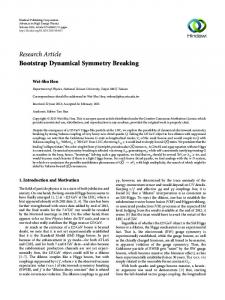
where hij (i, j = 1, 2, 3) be the matrix element of specific transition and ∆i be the detuning which vanishes at resonance. We note that from Eq.(1), the lambda system, which corresponds to the transition 1 ↔ 3 ↔ 2 shown in Fig.1a, can be described by the Hamiltonian with elements h21 = 0, h32 6= 0 and h31 6= 0. Similarly the vee model, characterized by the transition 3 ↔ 1 ↔ 2 shown in Fig.1b, corresponds to the elements h21 6= 0, h32 = 0 and h31 6= 0 and for the cascade model we have transition 1 ↔ 2 ↔ 3, we have h21 6= 0, h32 6= 0 and h31 = 0 respectively. Thus we have distinct Hamiltonian for three different configurations which can be read off from Eq.(1) shown in Fig.1. This definition, however, differs from the proposal advocated by Hioe and Eberly, who argued the order of the energy levels to be E1 < E3 < E2 for the lambda system, E2 < E3 < E1 for the vee system and E1 < E2 < E3 for the cascade system respectively [18,21,22]. In their scheme, the level-2 is always be the intermediary level which becomes the upper, lower and middle level to generate the lambda, vee and cascade configurations respectively. It is worth noting that, if we follow their scheme, these energy conditions map all three three-level configurations to a unique cascade Hamiltonian described by the matrix with elements h12 6= 0, h23 6= 0 and h13 = 0 in Eq.(1). Thus because of the similar structure of the model Hamiltonian, if we start formulating the solutions of the lambda, vee and cascade configurations, then it would led to same spectral feature. Furthermore, due to the same reason, the eight dimensional Bloch equation always remains same for all three models [18,22]. Both of these consequences go against the usual notion because wide range of coherent phenomena mentioned above arises essentially due to different class of the three-level configurations. Thus it is worth pursing to formulate a comprehensive approach, where we have distinct Hamiltonian for three configurations without altering the second level for each model. The problem of preparing multilevel atoms using one or more laser pulses is of considerable importance from experimental point of view. Thus the completeness of the study of the three-level systems requires the exact solution of these models to find the probability amplitudes of all levels, the effect of the field quantization on the population oscillation and, most importantly, the observation of the collapse and revival effect. In recent past, the three-level systems and its several ramifications were extensively covered in a general framework of the SU(N) group having N-levels [21-27,30,31]. Also, the semiclassical model [24,32,33] and its fully quantized version [23,34,35] are studied, but to our knowledge, the pursuit of the exact solutions of different three-level systems in the spirit of the theory of Electron Spin Resonance (ESR) model and JCM, are still to be facilitated 3

analytically. In a recent paper, we have studied the exact solutions of the equidistant cascade system interacting with the single mode classical and quantized field with different initial conditions [36]. It is shown that for the semiclassical model the Rabi oscillation exhibits a symmetric pattern of evolution, which is destroyed on quantization of the cavity field. We also show that this symmetry is restored by taking the cavity mode to be the coherent state indicating the proximity of the coherent state to the classical field. We have further studied the equidistant cascade four-level system and obtain similar conclusions [37]. To extend above studies for the lambda and vee models we note that the vee configuration can be obtained from the lambda configuration simply by inversion. However, it is worth noting that, the lambda configuration is associated with processes such as STIRAP [12], EIT [15,16] etc, while the vee configuration corresponds to the phenomena such as quantum jump [13], quantum zeno effect [14], quantum beat [3] etc indicating that both the processes are fundamentally different. It is therefore natural to examine the inversion symmetry between the models by comparing their Rabi oscillations and study the effect of the field quantization on that symmetry. The comparison shows that the inversion symmetry exhibited by the semiclassical models is completely spoiled on quantization of the cavity modes indicating the non-trivial role of the vacuum fluctuation in the symmetry breaking. The remaining part of the paper is organized as follows. In Section-II, we discuss the basic tenets of the SU(3) group necessary to develop the Hamiltonian of all possible three-level configurations. Section-III deals with the solution of the lambda model taking the two field modes as the classical fields and then in Section IV we proceed to solve the corresponding quantized version of the model using a novel Euler matrix formalism. Section-V and VI we present similar calculation for the vee model taking the mode fields to be first classical and then quantized respectively. In Section-VII we compare the population dynamics in both models and discuss its implications. Finally in Section-VIII we conclude our results.

II.The Models The most general Hamiltonian of a typical three-level configuration is given by Eq.(1) which contains several non-zero matrix elements showing all possible allowed transitions. To show how the SU(3) symmetry group provides a definite scheme of selection rule which forbids any one of the three transitions to give the Hamiltonian of a specific model, let us briefly recall the tenets of SU(3) group described by the Gell-Mann matrices, namely,

4









0 1 0    λ1 =  1 0 0  , 0 0 0 0 0 1    λ4 =  0 0 0  , 1 0 0 









1 0 0    λ3 =  0 −1 0  , 0 0 0 





0 0 0    λ6 =  0 0 1  , 0 1 0

0 0 −i    λ5 =  0 0 0  , i 0 0 



0 0 0    λ7 =   0 0 −i  , 0 i 0





0 −i 0    λ2 =  i 0 0  , 0 0 0

1 0 0   1  λ8 = √ 3   0 1 0 . 0 0 −2

(2)

These matrices follow the following commutation and anti-commutation relations [λi , λj ] = 2ifijk λk ,

{λi, λj } = 34 δij + 2dijk λk ,

(3)

respectively, where dijk and fijk (i, j = 1, 2, ..8) represent completely symmetric and completely antisymmetric structure constants which characterizes SU(3) group [39]. It is customary to define the shift operators T , U and V spin as T± = 21 (λ1 ± iλ2 ),

U± = 21 (λ6 ± iλ7 ),

V± = 12 (λ4 ± iλ5 ).

(4)

They satisfy the closed algebra [U+ , U− ] = U3 , [T3 , T± ] = ±2T± , [V3 , T± ] = ±T± , [U3 , T± ] = ∓T± , [T+ , V− ] = −U− , [T− , V+ ] = U+ ,

[V+ , V− ] = V3 , [T+ , T− ] = T3 , (5) [T3 , U± ] = ∓U± , [T3 , V± ] = ±V± , [V3 , U± ] = ±U± , [V3 , V± ] = ±2V± , [U3 , U± ] = ±2U± , [U3 , V± ] = ±V± , [T+ , U+ ] = V+ , [U+ , V− ] = T− , [T− , U− ] = −V− , [U− , V+ ] = −T+ , √ √ where the diagonal terms are T3 = λ3 , U3 = ( 3λ8 − λ3 )/2 and V3 = ( 3λ8 + λ3 )/2, respectively. The Hamiltonian of the semiclassical lambda model is given by HΛ = HΛI + HΛII ,

(6a)

where the unperturbed and interaction parts including the detuning terms are given by HΛI = h ¯ (Ω1 − ω1 − ω2 )V3 + h ¯ (Ω2 − ω1 − ω2 )T3 , and HΛII = h ¯ (∆Λ1 V3 + ∆Λ2 T3 )+ 5

(6b)

h ¯ κ1 (V+ exp(−iΩ1 t) + V− exp(iΩ1 t)) + h ¯ κ2 (T+ exp(−iΩ2 t) + T− exp(iΩ2 t)),

(6c)

respectively. In Eq.(6), Ωi (i = 1, 2) are the external frequencies of the bi-chromatic field, κi are the coupling parameters and h ¯ ω1 (= −E1 ), h ¯ ω2 (= −E2 ), h ¯ (ω2 + ω1 )(= E3 ) be the Λ respective energies of the three levels. ∆1 = (2ω1 + ω2 − Ω1 ) and ∆Λ2 = (ω1 + 2ω2 − Ω2 ) represent the respective detuning from the bi-chromatic external frequencies as shown in Fig.1. Proceeding in the same way, the semiclassical vee type three-level system can be written as V HV = HV I + HII ,

(7a)

HV ¯ (Ω1 − ω1 − ω2 )V3 + h ¯ (Ω2 − ω1 − ω2 )U3 , I =h

(7b)

where

and HV ¯ (∆V1 V3 + ∆V2 U3 )+ II = h h ¯ κ1 (V+ exp(−iΩ1 t) + V− exp(iΩ1 t)) + h ¯ κ2 (U+ exp(−iΩ2 t) + U− exp(iΩ2 t))

(7c)

where ∆V1 = (2ω1 + ω2 − Ω1 ) and ∆V2 = (2ω2 + ω1 − Ω2 ) be the detuning shown in Fig.2. Similarly the semiclassical cascade three-level model is given by HΞ = HΞI + HΞII ,

(8a)

HΞI = h ¯ (Ω1 + ω2 − ω1 )U3 + h ¯ (Ω2 + ω1 − ω2 )T3 ,

(8b)

where

and HΞII = h ¯ (∆Ξ1 U3 + ∆Ξ2 T3 )+ h ¯ κ1 (U+ exp(−iΩ1 t) + U− exp(iΩ1 t)) + h ¯ κ2 (T+ exp(−iΩ2 t) + T− exp(iΩ2 t))

(8c)

respectively with respective detuning ∆Ξ1 = (2ω1 − ω2 − Ω1 ) and ∆Ξ2 = (2ω2 − ω1 − Ω2 ). Taking the fields to be the quantized cavity fields, in the rotating wave approximation, the Hamiltonian of the quantized lambda configuration is given by Λ H Λ = HIΛ + HII ,

(9a)

where, 6

HIΛ = h ¯ (Ω2 − ω1 − ω2 )T3 + h ¯ (Ω1 − ω1 − ω2 )V3 +

2 P

j=1

Ωj a†j aj ,

(9b)

HIIΛ = h ¯ ∆Λ1 V3 + h ¯ ∆Λ2 T3 + h ¯ g1 (V+ a1 + V− a†1 ) + h ¯ g2 (T+ a2 + T− a†2 ),

(9c)

where a†i and ai (i = 1, 2) be the creation and annihilation operators of the cavity modes, gi be the coupling constants and Ωi be the mode frequencies. Proceeding in the similar pattern, the Hamiltonian of the quantized vee system is given by V H V = HIV + HII ,

(10a)

where, HIV = h ¯ (Ω2 − ω1 − ω2 )U3 + h ¯ (Ω1 − ω1 − ω2 )V3 +

2 P

j=1

Ωj a†j aj

(10b)

HIIV = h ¯ ∆V1 V3 + h ¯ ∆V2 U3 + h ¯ g1 (V+ a1 + V− a†1 ) + h ¯ g2 (U+ a2 + U− a†2 ),

(10c)

respectively. Similarly the Hamiltonian of the quantized cascade system reads Ξ H Ξ = HIΞ + HII ,

(11a)

where HIΞ = h ¯ (Ω2 − ω1 − ω2 )T3 + h ¯ (Ω1 − ω1 − ω2 )U3 +

2 P

j=1

Ωj a†j aj ,

(11b)

HIIΞ = h ¯ ∆Ξ1 U3 + h ¯ ∆Ξ2 T3 + h ¯ g1 (U+ a1 + U− a†1 ) + h ¯ g2 (T+ a2 + T− a†2 ).

(11c)

Using the algebra given in Eq.(5) and that of field operators, it is easy to check that [HIi , HIIi ] = 0 for ∆i1 = −∆i2 (i = Λ and V ) for the lambda and vee model and ∆Ξ1 = ∆Ξ2 for the cascade model which are identified as the two photon resonance condition and equal detuning conditions, respectively [18,21,22,24,26]. This ensures that each piece of the Hamiltonian has the simultaneous eigen functions. Thus we note that, unlike Ref.[18,21,22], precise formulation of the aforementioned three-level configurations require the use of a subset of Gell-Mann λi matrices rather than the use of all matrices. We now proceed to solve the lambda and vee configurations for the classical and the quantized field separately.

III.The semiclassical lambda system At zero detuning the Hamiltonian of the lambda type three-level system is given by 



h ¯ (ω1 + ω2 ) h ¯ κ2 exp[−iΩ2 t] h ¯ κ1 exp[−iΩ1 t]   Λ .  H = h ¯ κ2 exp[iΩ2 t] −¯ h ω2 0  h ¯ κ1 exp[iΩ1 t] 0 −¯ h ω1 7

(12)

The solution of the Schrodinger equation corresponding to Hamiltonian (12) is given by Ψ(t) = C1 (t) |1i + C2 (t) |2i + C3 (t) |3i

(13)

where C1 (t), C2 (t) and C3 (t) be the time-dependent normalized amplitudes of the lower, middle and upper levels with the respective basis states, 



0    |1i =  0  , 1





0    |2i =  1  , 0





1    |3i =  0  , 0

(14)

respectively. We now proceed to calculate the probability amplitudes of the three states. Substituting Eq.(13) in Schr¨odinger equation and equating the coefficients of |2i , |3i and |1i from both sides we obtain 3 = (ω2 + ω1 )C3 + κ1 exp(−iΩ1 t)C1 + κ2 exp(−iΩ2 t)C2 , i ∂C ∂t

(15a)

2 i ∂C = −ω2 C2 + κ2 exp(iΩ2 t)C3 , ∂t

(15b)

1 = −ω1 C1 + κ1 exp(iΩ1 t)C3 . i ∂C ∂t

(15c)

Let the solutions of Eqs.(15a-c) are of the following form, C1 = A1 exp(iS1 t),

(16a)

C2 = A2 exp(iS2 t),

(16b)

C3 = A3 exp(iS3 t),

(16c)

where Ai s’ are the time independent constants to be determined. Putting Eqs.(16a-c) in Eqs.(15a-c) we obtain (S3 + ω2 + ω1 )A3 + κ2 A2 + κ1 A1 = 0,

(17a)

(S3 + Ω2 − ω2 )A2 + κ2 A3 = 0,

(17b)

(S3 + Ω1 − ω1 )A1 + κ1 A3 = 0.

(17c)

In deriving Eqs.(17), the time independence of the amplitudes A3 , A2 and A1 are ensured by invoking the conditions S2 = S3 + Ω2 and S1 = S3 + Ω1 . At resonance, we have ∆Λ1 = 0 = −∆Λ2 i.e, (2ω2 + ω1 ) − Ω2 = 0 = (ω2 + 2ω1 ) − Ω1 and the solution of Eq.(17) yields S3 = −(ω2 + ω1 ) ± ∆, 8

(18a)

S3 = −(ω2 + ω1 ) where ∆ =

(18b)

q

κ21 + κ22 and we have three values of S2 and S1 namely S21 = ω2 , S22,3 = ω2 ± ∆,

(19a)

S11 = ω1 , S12,3 = ω1 ± ∆.

(19b)

Using Eqs.(18) and (19), Eq.(16) can be written as C3 (t) = A13 exp(−i(ω2 + ω1 )t) +A23 exp(i(−(ω2 + ω1 ) + ∆)t) + A33 exp(i(−(ω2 + ω1 ) − ∆)t),

(20a)

C2 (t) = A12 exp(iω2 t) + A22 exp(i(ω2 + ∆)t) + A32 (i(ω2 − ∆)t),

(20b)

C1 (t) = A11 exp(iω1 t) + A21 exp(i(ω1 + ∆)t) + A31 (i(ω1 − ∆)t),

(20c)

where Ai -s are the constants which can be calculated from the following initial conditions: Case-I: At t = 0 let the atom is in level-1, i.e. C1 (0) = 1, C2 (0) = 0, C3 (0) = 0. Using Eqns (15) and (20), the corresponding time-dependent probabilities of the three levels are |C3 (t)|2 =

κ21 ∆2

|C2 (t)|2 = 4 |C1 (t)|2 =

sin2 ∆t,

κ21 κ22 ∆4

(21a)

sin4 ∆t/2,

1 (κ22 ∆4

+ κ21 cos ∆t)2 .

(21b) (21c)

Case-II: If the atom is initially in level-2, i.e. C1 (0) = 0, C2 (0) = 1 and C3 (0) = 0, the probabilities of the three states are |C3 (t)|2 =

κ22 ∆2

|C2 (t)|2 =

1 (κ21 ∆4

|C1 (t)|2 = 4

sin2 ∆t,

κ21 κ22 ∆4

(22a)

+ κ22 cos ∆t)2 ,

sin4 ∆t/2.

(22b) (22c)

Case-III: When the atom is initially in level-3, i.e. C1 (0) = 0, C2 (0) = 0 and C3 (0) = 1, the time evolution of the probabilities of the three states are |C3 (t)|2 = cos2 ∆t, |C2 (t)|2 =

κ22 ∆2

(23a)

sin2 ∆t,

(23b) 9

κ2

|C1 (t)|2 = ∆12 sin2 ∆t. We now proceed to solve the quantized version of the above model.

(23c)

IV. The quantized lambda system We now consider the three-level lambda system interacting with a bi-chromatic quantized fields described by the Hamiltonian Eq.(9). At zero detuning the solution of the Hamiltonian is given by

|ΨΛ (t)i =

∞ P

n,m=0

[C1n−1,m+1 (t) |n − 1, m + 1, 1i + C2n,m (t) |n, m, 2i+C3n−1,m (t) |n − 1, m, 3i],

(24) where n and m represent the photon number corresponding to two modes of the bichromatic fields. This interaction Hamiltonian that couples the atom-field states |n − 1, m, 3i, |n, m, 2i and |n − 1, m + 1, 1i and forms the lambda configuration shown in Fig.1 is given by   √ √ 0 g2 n g1 m + 1   √ . (25) ¯ HIIΛ = h g n 0 0 2   √ 0 0 g1 m + 1 q

The eigenvalues of the Hamiltonian are given by λ± = ±¯ h ng22 + (m + 1)g12 and λ0 = 0(= Ω0 ), respectively with the corresponding dressed eigenstates 



(= ±¯ hΩnm )





|n − 1, m, 3i |nm, 3i     .  |nm, 2i  = Tn,m (g1 , g2 )  |n, m, 2i     |n − 1, m + 1, 1i |nm, 1i

(26)

In Eq.(26), the dressed states are constructed by rotating the bare states with the Euler matrix given by 



c3 c2 − c1 s2 s3 c3 s2 − c1 c2 s3 s 3 s 1    Tn,m (g1 , g2 ) =  −s3 c2 − c1 s2 c3 −s3 s2 + c1 c2 c3 c3 s1   s1 s2 −s1 c2 c1

(27)

where si = sin θi and ci = cos θi (i = 1, 2, 3). The elements of the matrix are found to 

Tn,m (g1 , g2 ) =

    

√1 2

0 − √12

n 2(ng22 +(m+1)g12 ) q m+1 g1 ng2 +(m+1)g 2 2 1 q n g2 2(ng2 +(m+1)g2 ) 2 1

g2

q

q

m+1 2(ng22 +(m+1)g12 ) q n −g2 ng2 +(m+1)g 2 2 1 q m+1 g1 2(ng2 +(m+1)g2 ) 2 1

g1

10



  ,  

(28)

with corresponding Euler angles, θ1 = arccos[ √

√

1+mg1 ], 2(1+m)g12 +2ng22

θ2 = − arccos[− √

√

ng2 ], (1+m)g12 +2ng22

θ3 = arccos[− √

√

2ng2 ]. (1+m)g12 +2ng22

(29) The time-dependent probability amplitudes of the three levels are given by C3n−1,m (0) e−iΩnm t 0 0 C3n−1,m (t)       −1    C2n,m (0)  0 e−iΩ0 t 0  C2n,m(t)  .  Tn,m (g1 , g2 )   = Tn,m (g1 , g2 )   n−1,m+1 n−1,m+1 iΩnm t C1 (0) 0 0 e C1 (t) 











(30) Now similar to the semiclassical model the probabilities corresponding to different initial conditions are: Case-IV: When the atom is initially in level-1, i.e, C1n−1,m+1 = 1, C2n,m = 0 and C3n−1,m = 0, the time-dependent atomic populations of the three states are given by n−1,m 2 (t) C3

=

|C2n,m (t)|2 = 4

(m+1)g12 Ω2nm

sin2 Ωnm t,

g12 g22 n(m+1) Ω4nm

n−1,m+1 2 C1 (t)

=

sin4 Ωnm t/2,

1 [ng22 Ω4nm

+ (m + 1)g12 cos Ωnm t]2 .

(31a) (31b) (31c)

Case-V: When the atom is initially in level-2, i.e, C1n−1,m+1 = 0, C2n,m = 1 and C3n−1,m = 0, the probabilities of three states are n−1,m 2 C3 (t)

|C2n,m (t)|2 =

=

ng22 Ω2nm

sin2 Ωnm t,

1 [(m Ω4nm

n−1,m+1 2 C1 (t)

=4

+ 1)g12 + ng22 cos Ωnm t]2 ,

g12 g22 n(m+1) Ω4nm

sin4 Ωmm t/2.

(32a) (32b) (32c)

Case-VI: If the atom is initially in level-3, then we have C1n−1,m+1 = 0, C2n,m = 0 and C3n−1,m+1 = 1 and the corresponding probabilities are n−1,m 2 C3 (t)

|C2n,m (t)|2 =

= cos2 Ωnm t, ng22 Ω2nm

n−1,m+1 2 C1 (t)

=

(33a)

sin2 Ωnm t,

(33b)

(m+1)g12 Ω2nm

(33c)

sin2 Ωnm t.

We now proceed to evaluate the population oscillations of different levels of the vee system with similar initial conditions. 11

V.The semiclassical vee system At zero detuning, the Hamiltonian of the semiclassical three-level vee system interacting with two-mode classical fields is given by 



h ¯ ω1 0 h ¯ κ1 exp[−iΩ1 t]   V H = 0 h ¯ ω2 h ¯ κ2 exp[−iΩ2 t]  .  h ¯ κ1 exp[iΩ1 t] h ¯ κ2 exp[iΩ2 t] −¯ h(ω1 + ω2 )

(34)

Let the solution of the Schrodinger equation corresponding to Eq.(34) is given by Ψ(t) = C1 (t) |1i + C2 (t) |2i + C3 (t) |3i ,

(35)

where C1 (t), C2 (t) and C3 (t) are the time-dependent normalized amplitudes with the basis vectors defined in Eqs.(13). To calculate the probability amplitudes of three states, substituting Eq.(35) into the Schr¨odinger equation we obtain 3 i ∂C = ω1 C3 + κ1 exp(−iΩ1 t)C1 , ∂t

(36a)

2 = ω2 C2 + κ2 exp(−iΩ2 t)C1 , i ∂C ∂t

(36b)

1 i ∂C = −(ω1 + ω2 )C1 + κ2 exp(iΩ2 t)C2 + κ1 exp(iΩ1 t)C3 . ∂t

(36c)

Let the solutions of Eqs.(36) are of the following form: C3 (t) = A3 exp(iS3 t),

(37a)

C2 (t) = A2 exp(iS2 t),

(37b)

C1 (t) = A1 exp(iS1 t),

(37c)

where Ai -s are the time independent constants to be determined from the boundary conditions. From Eq.(36) and Eq.(37) we obtain (S1 − Ω1 + ω1 )A3 + κ1 A1 = 0,

(38a)

(S1 − Ω2 + ω2 )A2 + κ2 A1 = 0,

(38b)

(S1 − ω2 − ω1 )A1 + κ2 A2 + κ1 A3 = 0.

(38c)

In deriving Eqs.(38), the time independence of the amplitudes A3 , A2 and A1 are ensured by invoking the conditions S2 = S1 − Ω2 and S3 = S1 − Ω1 . At resonance, ∆V1 = 0 = −∆V2 i.e. (2ω2 + ω1 ) − Ω2 = 0 = (ω2 + 2ω1 ) − Ω1 and the solutions of Eq.(38) are given by S1 = (ω1 + ω2 )

(39a) 12

S1 = (ω1 + ω2 ) ± ∆

(39b)

and we have three values of S2 and S3 S21 = −ω2 , S22,3 = −ω2 ± ∆

(40a)

S31 = −ω1 , S32,3 = −ω1 ± ∆.

(40b)

Using Eqs.(39) and (40), Eqs. (37) can be written as C3 (t) = A13 exp(−iω1 t) + A23 exp(−i(ω1 + ∆)t) + A33 (−i(ω1 − ∆)t),

(41a)

C2 (t) = A12 exp(−iω2 t) + A22 exp(−i(ω2 + ∆)t) + A32 (−i(ω2 − ∆)t),

(41b)

C1 (t) = A11 exp(i(ω2 + ω1 )t) +A21 exp(i((ω2 + ω1 ) + ∆)t) + A31 exp(i((ω2 + ω1 ) − ∆)t),

(41c),

where Ai -s are the constants which are calculated below from the various initial conditions. Case-I: Let us consider initially at t = 0, the atom is in level-1, i.e, C1 (0) = 1, C2 (0) = 0 and C3 (0) = 0. Using Eqs. (36) and (41), the time dependent probabilities of the three levels are given by |C3 (t)|2 =

κ21 ∆2

sin2 ∆t,

(42a)

|C2 (t)|2 =

κ22 ∆2

sin2 ∆t,

(42b)

|C1 (t)|2 = cos2 ∆t.

(42c)

Case-II: If the atom is initially in level-2, i.e, C1 (0) = 0, C2 (0) = 1 and C3 (0) = 0, the corresponding probabilities of the states are given by |C3 (t)|2 = 4

κ21 κ22 ∆4

sin4 ∆t/2,

|C2 (t)|2 =

1 (κ21 ∆4

|C1 (t)|2 =

κ22 ∆2

+ κ22 cos ∆t)2 ,

sin2 ∆t.

(43a) (43b) (43c)

Case-III: When the atom is initially in level-3, i.e, C1 (0) = 0, C2 (0) = 0 and C3 (0) = 1, we obtain the the occupation probabilities of the three states as follows: |C3 (t)|2 =

1 (κ22 ∆4

|C2 (t)|2 = 4

κ21 κ22 ∆4

+ κ21 cos ∆t)2 ,

sin4 ∆t/2, 13

(44a) (44b)

|C1 (t)|2 =

κ21 ∆2

sin2 ∆t.

(44c)

VI.The quantized vee system The eigenfunction of the quantized vee system described by the Hamiltonian in Eq.(10) is given by

|ΨV (t)i =

∞ P

n,m=0

[C1n+1,m (t) |n + 1, m, 1i + C2n,m (t) |n, m, 2i + C3n+1,m−1(t) |n + 1, m − 1, 3i]. (45)

Once again we note that the Hamiltonian couples the atom-field states |n + 1, m, 1i, |n, m, 2i and |n + 1, m − 1, 3i forming vee configuration depicted in Fig.2. The interaction part of the Hamiltonian (45) can also be expressed in the matrix form   √ 0 0 g1 m   √ ¯ HIIV = h (46) 0 0 g2 n + 1   , √ √ g1 m g2 n + 1 0 q

and the corresponding eigenvalues are λ± = ±¯ h mg12 + (n + 1)g22 0 respectively. The dressed eigenstate is given by 



(= ±¯ hΩnm ) and λ0 =





|n + 1, m − 1, 3i |nm, 3i     ,  |nm, 2i  = Tn,m  |n, m, 2i     |n + 1, m, 1i |nm, 1i

(47)

the rotation matrix is found to be 

Tn,m

g1 2((n+1)gm2 +mg2 )  2 1 q  n+1  =  −g2 (n+1)g2 +mg2 q

2



−g1

q

1

m 2((n+1)g22 +mg12 )

q

n+1 2((n+1)g22 +mg12 ) q g1 (n+1)gm2 +mg2 2 1 q n+1 −g2 2((n+1)g2 +mg2 ) 2 1

g2

√1 2

0 √1 2



  .  

(48)

The straightforward evaluation yields the various Euler angles are θ2 = arccos[− √

θ1 = − π4 ,

√ n+1g2 ], mg12 +(1+n)g22

θ3 = − π2 .

(49)

The time-dependent probability amplitudes of the three levels are given by C3n+1,m−1 (0) e−iΩnm t 0 0 C3n+1,m−1 (t)      −1    C2n,m (0) 0 e−iΩ0 t 0  C2n,m (t)   Tn,m   = Tn,m   C1n+1,m (0) 0 0 eiΩnm t C1n+1,m (t) 







14





 . 

(50)

Once again we proceed to calculate the probabilities for different initial conditions. Case-IV: Here we consider initially the atom is in level-1 i.e, C1n+1,m = 1, C2n,m = 0 and C3n+1,m−1 = 0. Using Eqs.(49) and (50) the time-dependent probabilities of the three levels are given by n+1,m−1 2 C3 (t)

|C2n,m (t)|2 = n+1,m 2 C1 (t)

=

mg12 Ω2nm

(n+1)g22 Ω2nm

sin2 Ωnm t,

sin2 Ωnm t,

= cos2 Ωnm t.

(51a) (51b) (51c)

Case-V: If the atom is initially in level-2 i.e, C3n+1,m−1 = 0, C2n,m = 1 and C1n+1,m = 0, then corresponding probabilities are n+1,m−1 2 C3 (t)

|C2n,m (t)|2 = n+1,m 2 C1 (t)

=4

g22 g12 (n+1)(m) Ω4mn

1 [mg12 Ω4nm

=

g22 (n+1) Ω2nm

sin4 Ωmn t/2,

(52a)

+ (n + 1)g22 cos Ωnm t]2 ,

(52b)

sin2 Ωnm t.

(52c)

Case-VI: Finally if the atom is initially in level-3 i.e, C1n+1,m = 0, C2n,m = 0 and C3n+1,m−1 = 1, then n+1,m−1 2 C3 (t) 2

|C2n,m (t)| = 4 n+1,m 2 C1 (t)

=

1 [mg12 Ω4nm

g22 g12 (n+1)(m) Ω4nm

=

mg12 Ω2nm

cos Ωnm t + (n + 1)g22]2 ,

sin4 Ωnm t/2,

sin2 Ωnm t.

(53a) (53b) (53c)

Finally we note that for large values of n and m, Case-IV, V and VI become identical to Case-I, II and III, respectively. This precisely shows the validity of the Bohr’s correspondence principle indicating the consistency of our approach.

VII.Numerical results and discussion Before going to show the numerical plots of the semiclassical and quantized lambda and vee systems, we first consider their analytical results. If we compare Case-I, II, III of both cases, we find that the probabilities in Case-I (Case-III)) of lambda system is the same as in Case-III (Case-I) of vee system except the populations of 1st and 3rd levels are interchanged. See Eqs.(21 & 44) and Eqs.(23 & 42) for detailed comparison. Also Case-II respective models are similar which is evident by comparing Eqs.(22 & 43). In 15

contrast, for the quantized model, Case-IV (Case-VI) of the lambda system is no longer same as in Case-VI (Case-IV) of the vee system. This breaking of symmetry is evident by comparing the analytical results, Eqs.(31 & 53), Eqs.(32 & 52) and Eqs.(32 & 51) respectively. Unlike previous case, also Case-V both the models are different which is evident from Eqs.(22 & 43). In what follows, we compare the probabilities of the semiclassical and quantized lambda and vee systems respectively. Fig.3 and 4 show the plots of the probabilities |C1i (t)|2 (blue line), |C2i (t)|2 (green line) and |C3i (t)|2 (red line) for the semiclassical lambda and vee models when the atom is initially at level-1 (Case-I), level-2 (Case-II) and level-3 (Case-III), respectively. The comparison of the plots shows that the pattern of the probability oscillation of the lambda system for Case-I shown in Fig.3a (Case-III in Fig.3c) is similar to that of Case-III shown in Fig.4c (Case-I in Fig.4a) of the vee system. More particularly we note that in all cases the oscillation of level-2 remains unchanged, while the oscillation of level-3 (level-1) of the lambda system for Case-I is identical to that of level-1 (level-3) of the vee system for Case-III. Furthermore, comparison of Fig.3b and Fig.4b for Case-II shows that the time evolution of the probabilities of level-2 of both systems also remains similar while those of level-3 and level-1 are interchanged. From the behaviour of the probability curve we can conclude that the lambda and vee configurations are essentially identical to each other as we can obtain one configuration from another simply by the inversion followed by the interchange of probabilities. For the quantized field, we first consider the time evolution of the probabilities taking the field is in a number state representation. In the number state representation, the vacuum Rabi oscillation corresponding to Case-IV, V and VI of the lambda and vee systems are shown in Fig.5 and Fig.6 respectively. We note that, unlike previous case, the Rabi oscillation for Case-IV shown in Fig.5a (Case-VI shown in Fig.5c) for the lambda model is no longer similar to Case-VI shown in Fig.6c (Case-IV shown in Fig.6a) for the vee model. Furthermore, we note that for Case-V, the oscillation patterns of Fig.5b is completely different from that of Fig.6b. In a word, for the quantized field, in contrast to the semiclassical case, the symmetry in the pattern of the vacuum Rabi oscillation in all cases is completely spoiled irrespective of the fact whether the system stays initially in any one of the three levels. The quantum origin of the breaking of the symmetric pattern of the Rabi oscillation is the following. We note that due to the appearance of the terms like (n + 1) or (m + 1), several elements in the probabilities given by Eqs.(31,32,33) for the lambda system and Eqs.(51,52,53) for the vee are non zero even at m = 0 and n = 0. We argue that the vacuum Rabi oscillation interferes with the probability oscillations of various levels and spoils their symmetric structure. Thus as a consequence of the vacuum fluctuation, the

16

symmetry of probability amplitudes of the dressed states of both models formed by the coherent superposition of the bare states is also lost. In the other word, the invertibility between the lambda and vee models exhibited for the classical field disappears as the direct consequence of the quantization of the cavity modes. Finally we consider the lambda and vee models interacting with the bi-chromatic quantized fields which are in the coherent state. The coherently averaged probabilities of level-3, level-2 and level-1 are given by

2

hP3 (t)iΛ =

P

n,m

Wn Wm C3n−1,m (t) ,

(54a)

hP2 (t)iΛ =

P

n,m

Wn Wm |C2n,m (t)|2 ,

(54b)

hP1 (t)iΛ =

P

n,m

Wn Wm C1n−1,m+1 (t) ,



2

(54c)



2

for the lambda system and hP3 (t)iV =

P

n,m

Wn Wm C3n+1,m−1 (t) ,

(55a)

hP2 (t)iV =

P

n,m

Wn Wm |C2n,m (t)|2 ,

(55b)

hP1 (t)iV =

P

Wn Wm C1n+1,m (t) ,

n,m



2

(55c)

1 n]¯ nn and Wm = m! exp[−m] ¯ m ¯ m with n ¯ and m ¯ for the vee system, where Wn = n!1 exp[−¯ be the mean photon numbers of the two quantized modes, respectively. Fig.7-9 display the numerical plots of Eq.(54) and Eq.(55) for Case-IV, V and VI respectively where the collapse and revival of the Rabi oscillation is clearly evident for large average photon numbers in both the fields. We note that in all cases, the collapse and revival of level-2 of both the systems are identical to each other. Furthermore, we note that the collapse and revival for lambda system initially in level-1 shown in Fig.7a, Fig.7b and Fig.7c (level-3 shown in Fig.9a, Fig.9b and Fig.9c) is the same as that of the vee system if it is initially in level-3 shown in Fig.7f, Fig.7e and Fig.7d (level-1 shown in Fig.9f, Fig.9e and Fig.9d) respectively. On the other hand, if the system is initially in level-2, the collapse and revival of the lambda systems shown in Fig.8a, Fig.8b and Fig.8c are identical to Fig.8f, Fig.8e and Fig.8d respectively for the vee system. This is precisely the situation what we obtained in case of the semiclassical model. Thus the symmetry broken in the case of the quantized model is restored back again indicating that the coherent state with large average photon number is very close to the classical state where the effect of field population in the vacuum level is almost zero. It is needless to say that the coherent state with very low average photon number in the field modes can not show the symmetric dynamics in lambda and vee systems.

17

VIII.Conclusion This paper presents the explicit construction of the Hamiltonians of the lambda, vee and cascade type of three-level configurations from the Gell-Mann matrices of SU(3) group and compares the exact solutions of the first two models with different initial conditions. It is shown that the Hamiltonians of different configurations of the three-level systems are different. We emphasize that there is a conceptual difference between our treatment and the existing approach by Hioe and Eberly [18,21,22]. These authors advocate the existence of different energy conditions which effectively leads to same cascade Hamiltonian (h21 6= 0, h32 6= 0 and h31 = 0 in Eq.(1)) having similar spectral feature irrespective of the configuration. We justify our approach by noting the fact that the two-photon condition and the equal detuning condition is a natural outcome of our analysis. For the lambda and vee models, the transition probabilities of the three levels for different initial conditions are calculated while taking the atom interacting with the bi-chromatic classical and quantized field respectively. It is shown that due to the vacuum fluctuation, the inversion symmetry exhibited by the semiclassical models is completely destroyed. In other words, the dynamics for the semiclassical lambda system can be completely obtained from the knowledge of the vee system and vice versa while such recovery is not possible if the field modes are quantized. The symmetry is restored again when the field modes are in the coherent state with large average photon number. Such breaking of the symmetric pattern of the quantum Rabi oscillation is not observed in case of the two-level Jaynes-Cummings model and therefore it is essentially a nontrivial feature of the multilevel systems which is manifested if the number of levels exceeds two. This investigation is a part of our sequel studies of the symmetry breaking effect for the equidistant cascade three-level and equidistant cascade four-level systems respectively [36,37]. Following the scheme of constructing of the model Hamiltonians, it is easy to show that we have different eight dimensional Bloch equations and non-linear constants for different configurations of the three-level systems and these issues will be considered elsewhere [40]. The breaking of the inversion symmetry of the lambda and vee models as a direct effect of the field quantization is an intricate issue especially in context with future cavity experiments with the multilevel systems.

Acknowledgement MRN thanks University Grants Commission and SS thanks Department of Science and Technology, New Delhi for partial financial support. We thank Dr T K Dey for discussions. SS is also thankful to S N Bose National Centre for Basic Sciences, Kolkata, for supporting his visit to the centre through the Visiting Associateship program. 18

References [1]

A Joshi and S V Lawande, Current Science 82 816 (2002); ibid 82 958 (2002)

[2]

L Hollberg, L Lugiato, A Oraevski, A sergienko and V Zadkov (Eds), J. Opt. B: Quan. Semiclass. Opt. 5 457 (2003)

[3]

A Nielsen, I L Chuang, Quantum Computation (Cambridge University Press, Cambridge 2002)

[4]

E T Jaynes and F W Cummings, Proc. IEEE, 51 89 (1963)

[5]

G Rempe, H Walther and N Klien, Phys Rev Lett 58 353 (1987)

[6]

R G Brewer and E L Hahn, Phys Rev A11 1641 (1975); P W Milloni and J H Eberly, J Chem Phys 68 1602 (1978), E M Belanov and I A Poluktov JETP 29 758 (1969); D Grischkowsky, M M T Loy and P F Liao, Phys Rev A12 2514 (1975) and references therein

[7]

B Sobolewska, Opt Commun 19 185 (1976), C Cohen-Tannoudji and S Raynaud, J Phys B10 365 (1977)

[8]

R M Whitley and C R Stroud Jr, Phys Rev A14 1498 (1976)

[9]

E Arimondo, Coherent Population Trapping in Laser Spectroscopy, Prog in Optics XXXV Edited by E Wolf (Elsevier Science, Amsterdam, 1996) p257.

[10]

C M Bowden and C C Sung, Phys Rev A18 1588 (1978)

[11]

T Mossberg, A Flusberg, R Kachru and S R Hartman, Phys Rev Lett 39 1523 (1984); T W Mossberg and S R Hartman, Phys Rev A 39 1271 (1981)

[12]

K Bergman, H Theuer and B W Shore, Rev Mod Phys 70 1003 (1998)

[13]

R J Cook and H J Kimble, Phys Rev Lett 54 1023 (1985); R J Cook, Phys Scr, T21 49 (1988)

[14]

B Misra and E C G Sudarshan, J Math Phys 18 756 (1977); C B Chiu, E C G Sudarshan and B Misra, Phys Rev D16 520 (1977); R J Cook, Phys Scr, T21 49 (1988)

[15]

S E Harris, Phys Today 50 36 (1997)

[16]

L V Lau, S E Harris, Z Dutton and C H Behroozi, Nature (London) 397 594 (1999) 19

[17]

C C Gerry and J H Eberly, Phys Rev A 42 6805 (1990)

[18]

F T Hioe and J H Eberly, Phys Rev A 25 2168 (1982)

[19]

H I Yoo and J H Eberly, Phys Rep 118 239 (1985)

[20]

B W Shore, P L Knight, J Mod Phy 40 1195 (1993)

[21]

F T Hioe and J H Eberly, Phys Rev Lett 47 838 (1981)

[22]

F T Hioe, Phys Rev A 28 879 (1983)

[23]

X Li and N Bei, Phys. Lett A 101 169 (1984)

[24]

J N Elgin, Phys Lett A80 140 (1980)

[25]

R J Cook, B W Shore, Phys Rev A20, 539 (1979)

[26]

F T Hioe and J H Eberly, Phys Rev 29 1164 (1984)

[27]

B Buck, C V Sukumar, J Phys A17 877 (1984)

[28]

T Nikajima, M Elk, Lambropoulos, Phys Rev A50 R913 (1994)

[29]

Tak-San Ho and Shih-I Chu, Phys Rev A31 659 (1985)

[30]

F Li, X Li, D L Lin and T F George, Phys Rev A40 5129 (1989) and references therein

[31]

F T Hioe, Phys Lett A99 150 (1983)

[32]

N V Kancheva, D Pushkarov and S Rashev, J Phys B: Mol Opt Phys 14 539 (1981)

[33]

N V Vitanov, J Phys B: Mol Opt Phys 31 709 (1998)

[34]

S Y Chu and D C Su, Phys Rev A25 3169 (2003)

[35]

N N Bogolubov Jr, F L Kien and A S Shumovsky, Phys Lett 101A (1984) 201; ibid, 107A (1985) 173

[36]

M R Nath, S Sen and G Gangopadhyay, Pramana-J Phys 61 1089 (2003) [quantph:0711.3884]

[37]

M R Nath, T K Dey, S Sen and G Gangopadhyay, Pramana-J Phys 70 141 (2008) [quant-ph:0712.2649v2] 20

[38]

M S Scully and M O Zubairy, Quantum optics, (Cambridge University Press, Cambridge, 1997) p16

[39]

D B Litchenberg, Unitary Symmetry and Elementary Particles (Academic Press, New York 1970)

[40]

M R Nath, S Sen and G Gangopadhyay, (In preparation)

21

∆1 Ω2

∆2 |3; m, n − 1 > |2; m, n >

Ω1

|1; m + 1, n − 1 >

Fig.1 : Lambda type transition

|3; m − 1, n + 1 >

∆1 Ω1 Ω2

∆2 |2; m, n > |1; m, n + 1 >

Fig.2 : Vee type transition

22

HaL

HbL

HcL

0 0

prob

1

prob

1

prob

1

0 0

50 t

0 0

50 t

50 t

[Fig.3]: The time evolution of the probabilities |C1 (t)|2 (blue line), |C2 (t)|2 (green

line) and |C3 (t)|2 (red line) of the semiclassical lambda system for Case-I, II and III

respectively with values κ1 = .2, κ2 = .1.

HaL

HbL

HcL

0 0

50

prob

1

prob

1

prob

1

0 0

t

50 t

0 0

50 t

[Fig.4]: The time variation of the probabilities |C1 (t)|2 (blue line), |C2 (t)|2 (green

line) and |C3 (t)|2 (red line) of the semiclassical vee system for Case-I, II and III

respectively with above values of κ1 , κ2 .

23

HaL

HbL

HcL

0 0

prob

1

prob

1

prob

1

0 0

50 t

0 0

50 t

50 t

[Fig.5]: The Rabi oscillation of the quantized lambda system when the fields are in the number state for Case-I, II and III, respectively with g1 = .2, g2 = .1, n = 1, m = 1.

HaL

HbL

HcL

0 0

50 t

prob

1

prob

1

prob

1

0 0

50 t

0 0

50 t

[Fig.6]: The Rabi oscillation of the quantized vee system when the fields are in the number states for Case-I, II and III, respectively for same values of g1 , g2 , n, m.

24

HaL

HbL

2000

0

HdL

1000 t

2000

0

1000 t

2000

0

HeL

0.7



0.7



1

1000 t

1000 t

2000

HfL



0

HcL

1



0.7



0.7

0

1000 t

2000

0

1000 t

2000

[Fig.7]: Figs.7a-c display the time-dependent collapse and revival phenomenon of level-3, level-2 and level-1 of the lambda system for Case-IV, while Figs.7d-f show that of the level-3, level-2 and level-1 respectively for of Case-VI of the vee system taking the field modes are in coherent states with n ¯ = 30 and m ¯ = 20.

25

HaL

HbL

2000

0

HdL

1000 t

2000

0

1000 t

2000

0

HeL

0.3



1



0.6

1000 t

1000 t

2000

HfL



0

HcL



0.6



1



0.3

0

1000 t

2000

0

1000 t

2000

[Fig.8]: Figs.8a-c display the time-dependent of collapse and revival of level-3, level2 and level-1 of the lambda system for Case-V while Figs.8d-f show that of level-3, level-2 and level-1 of the vee system for Case-V with the same values of n ¯ and m. ¯ as in Fig.7

26

HaL

HbL

2000

0

HdL

1000 t

2000

0

1000 t

2000

0

HeL

1



0.3



0.6

1000 t

1000 t

2000

HfL



0

HcL



0.6



0.3



1

0

1000 t

2000

0

1000 t

2000

[Fig.9]: Figs.9a-c display the time-dependent of collapse and revival of level-3, level2 and level-1 of the lambda system for Case-VI while Figs.9d-f show that for level-3, level-2 and level-1 respectively for the vee system for Case-IV with the same values of n ¯ and m ¯ as in Fig.7.

27