DYNAMICAL SYSTEMS AND DISCRETE METHODS FOR SOLVING ...

Applied Mathematics Reviews, World Sci. Pub. Co., vol. 1, (2000), 491-536

DYNAMICAL SYSTEMS AND DISCRETE METHODS FOR SOLVING NONLINEAR ILL-POSED PROBLEMS RUBEN G. AIRAPETYAN AND ALEXANDER G. RAMM

Contents 1. 2. 3. 4. 5. 6. 7. 8.

Introduction Continuous methods for well posed problems Discretization theorems for well-posed problems Nonlinear integral inequality Regularization procedure for ill-posed problems Discretization theorem for ill-posed problems Regularized continuous methods for monotone operators Regularized discrete methods for monotone operators 1. Introduction

The theme of this chapter is solving of nonlinear operator equation (1.1)

F (z) = 0,

F : H → H,

by establishing a relation between the limiting behavior for large times of the trajectories of dynamical systems in H and the solutions to equation (1.1) in a real Hilbert space H. We consider a real Hilbert space for the sake of simplicity, equation (1.1) in a complex Hilbert space can be treated similarly, and a part of results can be generalized to a Banach space. A standard approach to numerical solution of equation (1.1) consists of using one of the numerous iterative methods. These methods are also very useful for a theoretical investigation of problem (1.1). For some operators F they allow one to establish existence of a solution to problem (1.1), or existence and uniqueness theorems. In the iterative methods one chooses some initial approximation z0 and defines a sequence of points {zn }n=0,1,2,... having as a limit limn→∞ zn one of the solutions of equation (1.1). The choice of an initial point z0 is very important especially for problems solution to which is not unique. Usually the choice of z0 determines to what solution the iterative sequence converges. The simplest iterative method is the method of simple iteration defined as follows: (1.2)

zn = zn−1 − F (zn−1 ),

n = 1, 2, . . .

z0 is given. In the well-known Newton’s method ([14, 18, 19]) one constructs a sequence {zn } by the following formula: (1.3)

zn = zn−1 − [F 0 (zn−1 )]−1 F (zn−1 ), 1

n = 1, 2, . . . .

2

RUBEN G. AIRAPETYAN AND ALEXANDER G. RAMM

Here F 0 (h) is the Fréchet derivative of the operator F , defined at a point h ∈ H as a linear operator from H to H such that: (1.4)

F (h + ξ) − F (h) = F 0 (h)ξ + o(||ξ||).

Thus, an important condition for applicability of Newton’s method is invertibility of the Fréchet derivative operator F 0 . The important advantage of Newton’s method is the quadratic convergence to the solution in a neighborhood of this solution: (1.5)

||zn+1 − zn || ≤ const||zn − zn−1 ||2 .

In many cases when Newton’s method diverges one uses the damped Newton’s method: (1.6)

zn = zn−1 − ωn [F 0 (zn−1 )]−1 F (zn−1 ),

n = 1, 2, . . . ,

where ωn is an appropriately chosen sequence of positive numbers. In the gradient method one constructs an iterative sequence using the formula: (1.7)

zn = zn−1 − [F 0 (zn−1 )]∗ F (zn−1 ),

n = 1, 2, . . . .

The iterative methods mentioned above are widely known representatives of a large family of iterative methods. A detailed description of many iterative methods one can find in [19]. See also an approach to construction of iterative process for solving nonlinear equation proposed in [20, 21]. The applicability of iterative methods is established by various convergence theorems (see [14, 18, 19]), which specify assumptions on the operator F which guarantee convergence of the iterative sequence to a solution of equation (1.1). The proofs of convergence theorems for iterative methods are usually based on the contraction mapping principle. Another approach to solving problem (1.1) is based on a construction of a dynamical system with the trajectory starting from an initial approximation point z0 and having a solution to problem (1.1) as a limiting point. In [12] R. Courant proposed the dynamical system, which is a continuous analog of the gradient method, in the problem of minimization of some functionals. In [16] M.K. Gavurin proposed continuous Newton’s method and established the corresponding convergence theorem. In continuous Newton’s method one considers the following Cauchy problem for a nonlinear differential equation in a Hilbert space H: (1.8)

z(t) ˙ = −[F 0 (z(t))]−1 F (z(t)) z(0) = z0 ,

where z0 is some initial approximation point. In [25] E.P. Zhidkov and I.V. Puzynin applied continuous Newton’s method for solving nonlinear physical problems. Y. Alber used continuous methods for solving operator equations and variational inequalities ([6, 7, 8]). A modified continuous Newton’s method is proposed in [1, 3]. In this method one avoids numerically difficult inversion of the Fréchet derivative F 0 by solving an expanded system of nonlinear differential equation in Hilbert space. In [2, 3] one can find the applications of this method to some physical problems. The goal of this chapter is to develop a general approach to continuous analogs of discrete methods and to establish fairly general convergence theorems. This approach is based on an analysis of the solution to the Cauchy problem for a nonlinear differential equation in a Hilbert space. Such an analysis was done for well-posed and some ill-posed problems in [1, 4, 5], and was based on a usage of integral inequalities.

DYNAMICAL SYSTEMS AND DISCRETE METHODS FOR SOLVING NONLINEAR ILL-POSED PROBLEMS 3

Let z0 be an initial approximation for a solution to (1.1) and z(t) be the trajectory of an autonomous dynamical system: (1.9)

z(t) ˙ = Φ(z(t)),

0 ≤ t < ∞,

z(0) = z0 .

The main question investigated in this chapter is: Under what assumptions on operators F in (1.1) and Φ in (1.9) one can guarantee that: (i) Cauchy problem (1.9) is uniquely solvable for t ∈ [0, +∞), (ii) the solution z(t) tends to one of the solutions of (1.1) as t → ∞, (iii) there exists a step ω (or a sequence {ωn }) such that the corresponding discrete (iterative) method zn+1 = zn + ωΦ(zn ) (or zn+1 = zn + ωn Φ(zn )) produces the sequence {zn }, which converges to one of the solutions of (1.1). The answers are given in Theorems 2.2, 3.1 and Corollaries 1, 2. Thus an analysis of continuous processes is based on the investigation of the asymptotic behavior of nonlinear dynamical systems in Banach and Hilbert spaces. If a convergence theorem is proved for a continuous method, one can construct various discrete schemes generated by this continuous process. Thus construction of a discrete numerical scheme is divided into two parts: construction of the continuous process and numerical integration of the corresponding nonlinear differential equation in a Hilbert space. The main assumption in Theorems 2.2, 3.1 and Corollaries 1, 2 is that the Fréchet derivative F 0 of the operator F has a trivial null-space at the solution to (1.1). If F 0 has a nontrivial null-space at the solution to (1.1) then, in general, one can use the classical Newton method for solving of (1.1) only under some strong special assumptions on the operator F (see [9, 13]). In order to relax these assumptions and to construct numerical method for solving (1.1) when F 0 has a nontrivial nullspace at the solution to (1.1), one needs a regularized discrete Newton-like methods (see [6, 11, 15, 22, 24]). In this chapter we consider the continuous Newton’s method: (1.10)

z(t) ˙ = −[F 0 (z(t)) + ε(t)I]−1 [F (z(t)) + ε(t)(z(t) − z˜0 )],

z(0) = z0 ,

where ε(t) is a specially chosen positive function which tends to zero as t → +∞. Thus, in the framework of our general approach, instead of the Cauchy problem (1.9) for autonomous equation the following Cauchy problem for nonautonomous equation has to be considered: (1.11)

z(t) ˙ = Φ(z(t), t),

z(0) = z0 ,

where Φ is a nonlinear operator, Φ : H × [0, +∞) → H. An analysis of dynamical system (1.11) is more complicated. In this study we use new integral inequality (Theorem 4.2). Based on Theorem 4.2, a general convergence theorem for a regularized continuous process is proved (Theorem 5.1). Applying this theorem to the regularized Newton’s and simple iteration methods (for monotone operators) we obtain convergence theorems under less restrictive conditions on the equation than the theorems known for the corresponding discrete methods. Statements of these theorems contain some useful recommendations for the choice of a regularizing operator and estimate the rate of convergence of the regularized process. Convergence theorems for regularized continuous Newton-like methods are established in [4, 7, 22]. The applications of these scheme to GaussNewton-type methods for nonmonotone operators can be found in [4, 5].

4


Throughout this chapter the Hilbert space is assumed real-valued. 2. Continuous methods for well posed problems Let y be a solution to equation (1.1), z0 be some point in H, considered as an initial approximation to a solution to equation (1.1), and z(t) be some trajectory in H such that z(0) = z0 . Definition 2.1. We say that a trajectory z(t) converges to solution y of equation (1.1) exponentially if there exist positive constants c and c1 such that (2.1)

||z(t) − y|| ≤ c1 e−ct ||F (z0 )||,

||F (z(t))|| ≤ ||F (z0 )||e−ct .

Consider Cauchy problem (1.9). Examples of the choice of an operator Φ are given in Remark 1. Theorem 2.2. Assume that there exist some positive numbers r, c such that F , F 0 , and Φ are Fréchet differentiable and bounded in Br (z0 ) and the following conditions hold for every h ∈ Br (z0 ): (2.2)

(F 0 (h)Φ(h), F (h)) ≤ −c||F (h)||2 ,

and (2.3)

||Φ(h)|| ≤

rc ||F (h)||. ||F (z0 )||

Then 1) there exists a solution z = z(t), Br (z0 ) for all t ∈ [0, +∞); 2) there exists (2.4)

t ∈ [0, ∞), to problem (1.9) and z(t) ∈

lim z(t) = y,

t→+∞

y is a solution of problem (1.1) in Br (z0 ), and z(t) converges to y exponentially. Remark 2.3. a) Choosing Φ(h) = −[F 0 (h)]−1 F (h) one gets Continuous Newton’s method. In this case c = 1 and Theorem 2.2 yields the convergence theorem for Continuous Newton’s method ([16]); b) choosing Φ = −F , one gets a simple iteration method for which condition (2.2) means strict monotonicity of F ; c) Φ(h) = −[F 0 (h)]∗ F (h) corresponds to the gradient method. Proof of Theorem 2.2. From the Fréchet differentiability of Φ in Br (z0 ), we get the local existence of a solution of the problem (1.8). Then from (1.8) one gets: (2.5)

F 0 (z(t))z(t) ˙ = −F 0 (z(t))Φ(z(t).

From (2.5) denoting λ(t) = F (z(t)), one gets: ˙ (2.6) λ(t) = −F 0 (z(t))Φ(z(t), λ(0) = F (z0 ). Therefore, for sufficiently small t for which z(t) ∈ Br (z0 ), one can use estimate (2.2) and get: d ˙ ||λ(t)||2 = 2(λ(t), λ(t)) = −2(F 0 (z(t))Φ(z(t), F (z(t)) ≤ −2c||λ(t)||2 . dt Thus, the following estimate holds at least for sufficiently small t > 0: (2.7)

||λ(t)|| ≤ ||F (z0 )||e−ct .


For 0 ≤ t1 ≤ t2 one has: Zt2 ||z(t2 ) − z(t1 )|| ≤ ||

Zt2 z(s)ds|| ˙ ≤

t1

(2.8)

rc ≤ ||F (z0 )||

Zt2

||Φ(z(s))||ds t1

||λ(s)||ds ≤ r(e−ct1 − e−ct2 ) ≤ re−ct1 .

t1

Setting t1 = 0 and t2 = t, one concludes from (2.8) that z(t) ∈ Br (z0 ) for all t > 0. Now let t1 = t and t2 → +∞ in (2.8). Then one gets (2.9)

||z(t) − y|| ≤ re−ct ,

where y is defined in (2.4) and the limit in (2.4) does exist due to (2.8). The exponential convergence of z(t) to y follows now from (2.7) and (2.9). Remark 2.4. Note that in general the assumptions of Theorem 2.2 do not imply the uniqueness of a solution of equation (1.1) in Br (y). If (1.1) is not uniquely solvable then z(t) converges to one of its solutions. To establish convergence theorems for discrete methods we need a modified version of the statement of Theorem 2.2. We start with the following definition. Definition 2.5. Let y be a unique solution to equation (1.1) in some set M . M is called Φ-attractive set for y if for any z0 ∈ M the trajectory z(t) of the dynamical system (1.9) does not leave M and tends to y as t → +∞. If z(t) converges to y exponentially we call M an exponentially Φ-attractive set for y. If constants c and c1 in Definition 2.1 do not depend on a point z0 ∈ M we call M a uniformlyexponentially Φ-attractive set for y. Let us formulate a corollary to Theorem 2.2. Corollary 1. Assume that there exist some positive numbers r, c such that y is the unique solution to problem (1.1) in the ball Br (y), z0 ∈ Br (y), and the assumptions of Theorem2.2 are satisfied in Br (y). Then Br (y) is a uniformlyexponentially Φ-attractive set for y with c defined in (2.2) and r (2.10) c1 = . ||F (z0 )|| 3. Discretization theorems for well-posed problems Consider the following Cauchy problem: (3.1)

z(t) ˙ = Φ(z(t)),

z(0) = z0 ,

and the corresponding discrete process: (3.2)

zn+1 = zn + ωΦ(zn ).

Theorem 3.1. Let Br (y) be a uniformly-exponentially Φ-attractive set for y for some r > 0 such that r ≥ c1 ||F (z0 )||, where c1 is the same as in Definition 2.1, z0 ∈ Br (y). Assume that (1) F and Φ are Fréchet differentiable in Br (y), and (3.3)

||Φ(h)|| ≤ N0 ||F (h)||, ||F 0 (h)|| ≤ N1 , ||Φ0 (h)|| ≤ N2 for h ∈ Br (y),

6


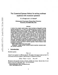
Figure 1. Discretization scheme of a continuous process. (2) c2 and ω are some positive constants satisfying the following inequalities: (3.4)

(c1 e−cω + N0 N2 ω 2 )||F (z0 )|| ≤ re−c2 ω ,

(3.5)

e−cω + N0 N1 N2 ω 2 ≤ e−c2 ω .

Then all {zn }, n = 1, 2, . . . , defined by formula (3.2) belong to the ball Br (y) and (3.6)

||zn − y|| ≤ re−c2 nω ,

||F (zn )|| ≤ ||F (z0 )||e−c2 nω ,

n = 0, 1, 2, . . . .

Proof of Theorem 3.1 The idea of the proof is illustrated in Figure1. Let z0 be an initial approximation point. Since Br (y) is an exponentially attractive set for y integral curve ψ0 (t) of equation (3.1) connects z0 with y. Let ω be a stepsize. Consider points ψ1 (ω) and z1 defined by (3.1) and (3.2) correspondingly. The point ψ1 (ω) is located on an integral curve and the point z1 is located on a tangent line to this integral curve passing through z0 . Since ψ1 (t) converges exponentially to y and the distance between ψ1 (ω) and z1 decreases as ω 2 for ω → 0, one shows that for a sufficiently small step ω, z1 is closer to y than z0 . Therefore z1 also belongs to Br (y). Moreover using the triangle inequality one can estimate the distance between z1 and y. Then take the integral curve ψ2 (t), which connects z1 with y, points ψ2 (ω) and z2 , show that z2 belongs to Br (y), and estimate the distance between z2 and y. Repeating this process one estimates the distance between {zn } and y and shows that this distance exponentially tends to zero. We prove (3.6) using mathematical induction. For n = 0 conditions (3.6) are satisfied. Assume that (3.6) are satisfied for n = m − 1. Denote by ψm (t) the solution to the following Cauchy problem: (3.7)

z(t) ˙ = Φ(z(t)),

0 < t ≤ ω,

z(0) = zm−1 .

Then one has: (3.8)

||zm − y|| ≤ ||ψm (ω) − y|| + ||ψm (ω) − zm ||.

Since Br (y) is a uniform-exponentially Φ-attractive set for y one gets: (3.9)

||F (ψm (t))|| ≤ ||F (zm−1 )||e−ct ,

t ∈ [0, ω],

and (3.10)

||ψm (ω) − y|| ≤ c1 e−cω ||F (zm−1 )|| ≤ c1 e−cω e−c2 ω(m−1) ||F (z0 )||.

From (3.1) and (3.2) one obtains: Zω ψm (ω) − zm =

Zω [Φ(z(τ )) − Φ(zm−1 )]dτ =

0

dτ 0

Zω (3.11)

Z1

=

Z1 τ dτ

0

0

Φ0 (z(sτ ))z(sτ ˙ )ds

0

d Φ(z(sτ ))ds = ds


Therefore Zω (3.12)

||ψm (ω) − zm || ≤ ω

||Φ0 (z(s))|| ||Φ(z(s))|| ds.

0

Using (3.9) one gets: Zω ||ψm (ω) − zm || ≤ ωN0 N2

||F (z(s))||ds 0

(3.13)

≤ ω 2 N0 N2 ||F (zm−1 )|| ≤ ω 2 N0 N2 e−c2 ω(m−1) ||F (z0 )||.

From (3.8), (3.10), and (3.13) one gets: (3.14)

||zm − y|| ≤ (c1 e−cω e−c2 ω(m−1) + ω 2 N0 N2 e−c2 ω(m−1) )||F (z0 )||.

Using condition (2.10) one obtains: (3.15)

||zm − y|| ≤ re−c2 mω .

Also ||F (zm )|| ≤ ||F (ψm (ω))|| + N1 ||ψm (ω) − zm || ≤ e−cω ||F (zm−1 )|| +ω 2 N0 N1 N2 e−c2 ω(m−1) ||F (z0 )|| ≤ e−c2 ω(m−1) (e−cω + ω 2 N0 N1 N2 )||F (z0 )|| (3.16)

≤ (e−cω + ω 2 N0 N1 N2 )e−c2 ω(m−1) ||F (z0 )||.

From (3.16) and (3.5) one gets: (3.17)

||F (zm )|| ≤ ||F (z0 )||e−c2 mω .

Thus the estimate (2.10) and (3.5) hold also for n = m. Theorem 3.1 is proved. Corollary 2. Assume that there exist some positive numbers r, c such that: (1) y is the unique solution to problem (1.1) in the ball Br (y), and an initial approximation point z0 ∈ Br (y), (2) the assumptions of Theorem2.2 are satisfied in Br (y), (3) (3.18)

||F 0 (h)|| ≤ N1 , ||Φ0 (h)|| ≤ N2

for

h ∈ Br (y),

(4) c2 and ω are some positive constants satisfying the following inequality: rN1 −cω 2 ≤ e−c2 ω , (3.19) e + cN2 ω max 1, ||F (z0 )|| (5) z0 is an initial approximation point and the sequence {zn }, n = 1, 2, . . . , is defined recursively: (3.20)

zn = zn−1 + ωΦ(zn−1 ),

Then all {zn }, n = 1, 2, . . . , belong to the ball Br (y) and (3.21)

||zn − y|| ≤ re−c2 nω ,

||F (zn )|| ≤ ||F (z0 )||e−c2 nω ,

n = 0, 1, 2, . . . .

Proof of Corollary 2. Since the assumptions of Theorem 2.2 are satisfied in Br (y), choosing rc (3.22) N0 = ||F (z0 )||

8


one gets the first inequality in (3.3) from (2.3). The second and the third inequalities in (3.3) follow from (3.18). From Corollary 1 one gets that Br (y) is a uniformly-exponentially Φ-attractive set for y with c defined in condition (2.2) and r (3.23) c1 = . ||F (z0 )|| For such N0 and c1 condition (3.19) is equivalent to conditions (2.10) and (3.5). To finish the proof one refers to Theorem 3.1. 4. Nonlinear integral inequality The main result of this section is Theorem 4.2 which is used throughout the paper. The following lemma is a version of some known results concerning integral inequalities (see e.g. Theorem 22.1 in [23]). For convenience of the reader and to make the presentation essentially self-contained we include a proof. Lemma 4.1. Let f (t, w), g(t, u) be continuous on region [0, T ) × D (D ⊂ R, T ≤ ∞) and f (t, w) ≤ g(t, u) if w ≤ u, t ∈ (0, T ), w, u ∈ D. Assume that g(t, u) is such that the Cauchy problem (4.1)

u˙ = g(t, u),

u0 ∈ D

u(0) = u0 ,

has a unique solution. If (4.2)

w˙ ≤ f (t, w),

w(0) = w0 ≤ u0 ,

w0 ∈ D,

then u(t) ≥ w(t) for all t for which u(t) and w(t) are defined. Proof of Lemma 4.1 ˙ ≤ Step 1. Suppose first f (t, w) < g(t, u), if w ≤ u. Since w0 ≤ u0 and w(0) f (t, w0 ) < g(t, u0 ) = u(0), ˙ there exists δ > 0 such that u(t) > w(t) on (0, δ]. Assume that for some t1 > δ one has u(t1 ) < w(t1 ). Then for some t2 < t1 one has u(t2 ) = w(t2 )

and u(t) < w(t)

for t ∈ (t2 , t1 ].

One gets w(t ˙ 2 ) ≥ u(t ˙ 2 ) = g(t, u(t2 )) > f (t, w(t2 )) ≥ w(t ˙ 2 ). This contradiction proves that there is no point t2 such that u(t2 ) = w(t2 ). Step 2. Now consider the case f (t, w) ≤ g(t, u), if w ≤ u. Define u˙ n = g(t, un ) + εn ,

un (0) = u0 ,

εn > 0,

n = 0, 1, ...,

where εn tends monotonically to zero. Then w˙ ≤ f (t, w) ≤ g(t, u) < g(t, u) + εn ,

w ≤ u.

By Step 1 un (t) ≥ w(t), n = 0, 1, ... . Fix an arbitrary compact set [0, T1 ], 0 < T1 < T. Zt (4.3) un (t) = u0 + g(τ, un (τ ))dτ + εn t. 0

Since g(t, u) is continuous, the sequence {un } is uniformly bounded and equicontinuous on [0, T1 ]. Therefore there exists a subsequence {unk } which converges


uniformly to a continuous function u(t). By continuity of g(t, u) we can pass to the limit in (4.3) and get Zt (4.4)

u(t) = u0 +

g(τ, u(τ ))dτ,

t ∈ [0, T1 ].

0

Since T1 is arbitrary (4.4) is equivalent to the initial Cauchy problem that has a unique solution. The inequality unk (t) ≥ w(t), k = 0, 1, ... implies u(t) ≥ w(t). If the solution to the Cauchy problem (4.1) is not unique, the inequality w(t) ≤ u(t) holds for the maximal solution to (4.1). The following theorem is a key to the basic result, namely to Theorem 5.1. Theorem 4.2. Let γ(t), σ(t), β(t) ∈ C[t0 , ∞) for some real number t0 . If there exists a positive function µ(t) ∈ C 1 [t0 , ∞) such that µ(t) ˙ 1 µ(t) ˙ µ(t) γ(t) − , β(t) ≤ γ(t) − , (4.5) 0 ≤ σ(t) ≤ 2 µ(t) 2µ(t) µ(t) then a nonnegative solution to the following inequalities: (4.6)

v(t) ˙ ≤ −γ(t)v(t) + σ(t)v 2 (t) + β(t),

v(t0 )
0. In Theorem 4.2 the term −γ(t)v(t) + σ(t)v 2 (t) (which is analogous to some extent to the term −A(t)ψ(v(t))) can change sign. Our Theorem 4.2 is not covered by the result in [8]. In particular, in Theorem 4.2 an analog of ψ(v), for the case γ(t) = σ(t) = A(t), is the function ψ(v) := v − v 2 . This function goes to −∞ as v goes to +∞, so it does not satisfy the positivity condition imposed in [8]. Unlike in the case of Bihari integral inequality ([10]) one cannot separate variables in the right hand side of the first inequality (4.6) and estimate v(t) by a solution of the Cauchy problem for a differential equation with separating variables. The proof below is based on a special choice of the solution to the Riccati equation majorizing a solution of inequality (4.6). Proof of Theorem 4.2. Denote: (4.9)

Rt

w(t) := v(t)e

t0

γ(s)ds

,

then (4.6) implies: (4.10)

w(t) ˙ ≤ a(t)w2 (t) + b(t),

w(t0 ) = v(t0 ),

10


where −

a(t) = σ(t)e Consider Riccati’s equation: (4.11)

Rt t0

γ(s)ds

u(t) ˙ =

,

Rt

b(t) = β(t)e

t0

γ(s)ds

.

f˙(t) 2 g(t) ˙ u (t) − . g(t) f (t)

One can check by a direct calculation that the the solution to problem (4.11) is given by the following formula [17, eq. 1.33]: " !#−1 Z t g(t) f˙(s) 2 (4.12) u(t) = − + f (t) C − ds . 2 f (t) t0 g(s)f (s) Define f and g as follows: (4.13)

− 12

1

f (t) := µ 2 (t)e

Rt t0

γ(s)ds

,

1

1

g(t) := −µ− 2 (t)e 2

Rt t0

γ(s)ds

,

and consider the Cauchy problem for equation (4.11) with the initial condition u(t0 ) = v(t0 ). Then C in (4.12) takes the form: 1 C= . µ(t0 )v(t0 ) − 1 From (4.5) one gets a(t) ≤

f˙(t) , g(t)

b(t) ≤ −

g(t) ˙ . f (t)

Since f g = −1 one has: Z t Z t ˙ Z f˙(s) f (s) 1 t µ(s) ˙ ds = − ds = γ(s) − ds. 2 2 t0 µ(s) t0 g(s)f (s) t0 f (s) Thus Rt

(4.14)

u(t) =

e

t0

γ(s)ds

µ(t)

"

1−

1 1 + 1 − µ(t0 )v(t0 ) 2

Z t t0

µ(s) ˙ γ(s) − µ(s)

−1 #

ds

.

It follows from conditions (4.5) and from the second inequality in (4.6) that the solution to problem (4.11) exists for all t ∈ [0, ∞) and the following inequality holds with ν(t) defined by (4.8): 1 > 1 − ν(t) ≥ µ(t0 )v(t0 ).

(4.15)

From Lemma 4.1 and from formula (4.14) one gets: (4.16)

Rt

v(t)e

t0

γ(s)ds

:= w(t) ≤ u(t) =

1 − ν(t) Rtt γ(s)ds 1 Rtt γ(s)ds e 0 < e 0 , µ(t) µ(t)

and thus estimate (4.7) is proved. To illustrate conditions of Theorem 4.2 consider the following examples of functions γ, σ, β, satisfying (4.5) for t0 = 0. Example 4.4. Let (4.17)

γ(t) = c1 (1 + t)ν1 ,

σ(t) = c2 (1 + t)ν2 ,

β(t) = c3 (1 + t)ν3 ,

where c2 > 0, c3 > 0. Choose µ(t) := c(1 + t)ν , c > 0. From (4.5), (4.6) one gets the following conditions cc1 cν c2 ≤ (1 + t)ν+ν1 −ν2 − (1 + t)ν−1−ν2 , 2 2


(4.18)

c3 ≤

c1 ν (1 + t)ν1 −ν−ν3 − (1 + t)−ν−1−ν3 , 2c 2c

cv(0) < 1.

Thus one obtains the following conditions: ν1 ≥ −1,

(4.19)

ν2 − ν1 ≤ ν ≤ ν1 − ν3 ,

and (4.20)

c1 > ν,

c1 − ν 2c2 ≤c≤ , c1 − ν 2c3

cv(0) < 1.

Therefore for such γ, σ, β a function µ with the desired properties exists if ν1 ≥ −1,

(4.21)

ν2 + ν3 ≤ 2ν1 ,

and (4.22)

c1 > ν2 − ν1 ,

√ 2 c2 c3 ≤ c1 + ν1 − ν2 ,

2c2 v(0) < c1 + ν1 − ν2 .

2c2 In this case one can choose ν = ν2 − ν1 , c = c1 +ν . However in order to have 1 −ν2 v(t) → 0 as t → +∞ (the case of interest in Theorem 5.1) one needs the following conditions:

ν1 ≥ −1,

(4.23)

ν2 + ν3 ≤ 2ν1 ,

ν1 > ν3 ,

and √ 2 c2 c3 ≤ c1 ,

c1 > ν2 − ν1 ,

(4.24)

2c2 v(0) < c1 .

Example 4.5. If γ(t) = γ0 ,

σ(t) = σ0 eνt ,

β(t) = β0 e−νt ,

µ(t) = µ0 eνt ,

then conditions (4.5), (4.6) are satisfied if 0 ≤ σ0 ≤

µ0 (γ0 − ν), 2

β0 ≤

1 (γ0 − ν), 2µ0

µ0 v(0) < 1.

Example 4.6. Here and throughout the paper log stands for the natural logarithm. For some t1 > 0 1

γ(t) = p

log(t + t1 )

,

µ(t) = c log(t + t1 ),

conditions (4.5), (4.6) are satisfied if c p 1 0 ≤ σ(t) ≤ log(t + t1 ) − , 2 t + t1 1 β(t) ≤ 2 2c log (t + t1 )

1 log(t + t1 ) − t + t1

p

,

v(0)c log t1 < 1.

In all considered examples µ(t) can tend to infinity as t → +∞ and provide a decay of a nonnegative solution to integral inequality (4.6) even if σ(t) tends to infinity. Moreover in the first and the third examples v(t) tends to zero as t → +∞ when γ(t) → 0 and σ(t) → +∞.

12


5. Regularization procedure for ill-posed problems In the well-posed case (when the Fréchet derivative F 0 of the operator F is a bijection in a neighborhood of the solution of equation (1.1)) in order to solve equation (1.1) one can use the following continuous processes: • simple iteration method: z(t) ˙ = −F (z(t)),

(5.1)

z(0) = z0 ∈ H,

• Newton’s method: z(t) ˙ = −[F 0 (z(t))]−1 F (z(t)),

(5.2)

z(0) = z0 ∈ H.

0

However if F is not continuously invertible (ill-posed case) one has to replace the Cauchy problems (5.1) and (5.2) by the corresponding regularized Cauchy problems (see [4, 5, 6]): • regularized simple iteration method: (5.3)

z(t) ˙ = −[F (z(t)) + ε(t)(z(t) − z˜0 )],

z(0) = z0 ∈ H,

• regularized Newton’s method: (5.4)

z(t) ˙ = −[F 0 (z(t)) + ε(t)I]−1 [F (z(t)) + ε(t)(z(t) − z˜0 )],

z(0) = z0 ∈ H.

Here z˜0 ∈ H is some element, ε(t) > 0 is a suitable function, with the properties specified in Theorems 7.12 and 7.22, and I is the identity operator. The equations in (5.3) and (5.4) are no longer autonomous. Our goal is to develop a uniform approach to such regularized methods. Let us consider the Cauchy problem: (5.5)

z(t) ˙ = Φ(z(t), t),

z(0) = z0 ∈ H,

with an operator Φ : H × [0, ∞) → H. Let y be a solution to equation (1.1) (as it was mentioned in Introduction, we assume that this equation is solvable). Denote: BR (y) := {h : h ∈ H, ||h−y|| < R}. Theorem 5.1. Assume that there exists r > 0 such that Φ(h, t) is Fréchet differentiable with respect to h in the ball B2r (y) for any t ∈ [0, ∞) and satisfy the following condition: there exists a differentiable function x(t), x : [0, +∞) → Br (y), such that for any h ∈ B2r (y), t ∈ [0, +∞) (5.6)

(Φ(h, t), h − x(t)) ≤ α(t)||h − x(t)|| − γ(t)||h − x(t)||2 + σ(t)||h − x(t)||3 ,

where α(t) is a continuous function, α(t) ≥ 0, γ(t) and σ(t) satisfy conditions (4.5) of Theorem 4.2 with (5.7)

β(t) := ||x(t)|| ˙ + α(t),

µ(t) in (4.5) tends to +∞ as t → +∞, and (5.8)

||z0 − x(0)||
0. By Theorem 4.2 using (5.8) one obtains (5.14)

||z(t) − x(t)|| ≤

1 ≤ r, µ(t)

for

t ∈ [0, T ).

Thus, since x(t) ∈ Br (y), one gets (5.15)

||z(t) − y|| ≤ ||z(t) − x(t)|| + ||x(t) − y|| < 2r,

for

t ∈ [0, T ).

Therefore there exists a sequence {tn } → T such that {z(tn )} converges weakly to some z ∗ . From equation (5.5) one derives the uniform boundedness of the norm ||z(t)|| ˙ on [0, T ) since ||Φ(z(t), t)|| ≤ const < ∞ for ||z(t)|| ≤ const and 0 ≤ t ≤ const. Thus there exists limt→T ||z(t) − z ∗ || = 0. Since (5.16)

||z ∗ − y|| ≤ ||z ∗ − x(T )|| + ||x(T ) − y|| < 2r

for

t ∈ [0, T ),

the conditions for the unique local solvability of the Cauchy problem for equation (5.5) with initial condition z(T ) = z ∗ are satisfied. Therefore one can continue the solution to (5.5) through the point T . This contradicts the assumption of maximality of T , thus T = +∞. Moreover, from (4.7) one gets: (5.17)

lim ||z(t) − x(t)|| ≤ lim

t→+∞

t→+∞

1 = 0. µ(t)

14


In order to establish the discretization theorem in the next section we need to estimate ||Φ|| along the trajectory z(t). The following theorem gives such an estimate. Theorem 5.3. Let the assumptions of Theorem 5.1 hold and z(t) solve problem (5.5). Assume that the following two conditions hold: (1) for any h belonging to the trajectory z(t), Φ(h, t) is differentiable with respect to t and the following two inequalities hold: ! (5.18)

(5.19)

(Φ0 (h, t)ξ, ξ) ≤

−a1 (t) + a2 (t)||Φ(h, t)|| ||ξ||2 for any ξ ∈ H,

∂Φ ≤ β1 (t) + b1 (t)||Φ(h, t)|| + b2 (t)||Φ(h, t)||2 , (h, t) ∂t

where Φ0 (h, t) is the Fréchet derivative with respect to h, ∂Φ/∂t is the derivative with respect to t, a1 (t), a2 (t), β1 (t), b1 (t), and b2 (t) are continuous functions; (2) the functions γ1 (t) := a1 (t) − b1 (t), σ1 (t) := a2 (t) + b2 (t) and β1 (t) are continuous and satisfy conditions (4.5) of Theorem 4.2 with v1 (0) := ||Φ(z0 , 0)|| < 1 µ1 (0) and with µ1 (t) > 0, which tends to +∞ as t → +∞. Then the following estimate holds: ||Φ(z(t), t)|| ≤

(5.20)

1 . µ1 (t)

Proof of Theorem 5.3. Denote v1 (t) := ||Φ(z(t), t)||. Recall that H is a real Hilbert space. From (5.5) one gets: d ∂Φ dv1 0 (5.21) v1 = Φ(z(t), t), Φ(z(t), t) = + Φ (z(t), t)z(t), ˙ Φ(z(t), t) . dt dt ∂t From (5.21) and (5.5) one gets: (5.22)

dv1 v1 = dt

! ∂Φ 0 Φ (z(t), t)Φ(z(t), t), Φ(z(t), t) + , Φ(z(t), t) . ∂t

Using (5.18) and (5.19) one obtains from (5.22) the following inequality: v1 v˙ 1 ≤ (−a1 (t) + a2 (t)v1 )v12 + (β1 (t) + b1 (t)v1 + b2 (t)v12 )v1 , or (5.23)

v˙ 1 ≤ β1 + (b1 − a1 )v1 + (a2 + b2 )v12 = β1 − γ1 v1 + σ1 v12 ,

where γ1 (t) = a1 (t) − b1 (t) and σ1 (t) = a2 (t) + b2 (t). It follows from the assumptions of Theorem 5.3 that v1 (t) satisfies the integral inequality: dv1 ≤ −γ1 (t)v1 (t) + σ1 (t)v12 (t) + β1 (t). dt To finish the proof of Theorem 5.3 one uses Theorem 4.2.

(5.24)


6. Discretization theorem for ill-posed problems The theorem of this section gives an answer to the following question: under what assumptions on Φ and {ωn } the convergence of a continuous process (6.1)

z(t) ˙ = Φ(z(t), t),

z(0) = z0 ,

implies the convergence of the corresponding discrete process (6.2) (6.3)

zn = zn−1 + ωn Φ(zn−1 , tn−1 ), tn = tn−1 + ωn ,

t0 = 0,

n = 1, 2, . . . ,

where z0 in (94) is the same as in (6.1). Theorem 6.1. Let Φ satisfy conditions of Theorems 5.1 and 5.3 with a function x(t), which tends to y as t → +∞. Assume that (1) (6.4)

||Φ0 (h, t)|| ≤ a3 (t) + a2 (t)||Φ(h, t)||,

where a3 (t) is a nonnegative continuous function and a2 (t) is the same as in Theorem 5.3; (2) the sequence {zn } is defined by formulas (6.2) and (6.3); (3) (6.5)

A=

sup (a1 (t) + a3 (t)) < +∞, t∈[0,+∞)

where a1 (t) is defined in (5.18); (4) (6.6)

0 < ωn ≤

1 , A

∞ X

ωn = ∞;

n=1

(5) ωn µ1 (tn ) < , νn (ωn ) µ(tn )

(6.7)

(6.8)

where Z 1 1 1 t µ(s) ˙ = + γ(s) − ds, νn (t) 1 − µ(tn−1 )||zn−1 − x(tn−1 )|| 2 tn−1 µ(s)

the continuous positive functions µ(t), µ1 (t) are defined in Theorems 5.1 and 5.3; (6) the function µ1 (t) is monotonically increasing. Then the following conclusions hold: i) all zn , n = 1, 2, . . . , belong to the ball B2r (y); ii) 1 (6.9) ||zn − x(tn )|| < ; µ(tn ) iii) (6.10)

tn → +∞,

1 →0 µ(tn )

as

n → ∞;

16


iv) lim ||zn − y|| = 0.

(6.11)

n→∞

Proof of Theorem 6.1. Statements (6.10) follow from (6.6) and from the assumption that µ1 (t) → ∞ as 1 t → ∞. We prove (6.9) by induction. It follows from (5.8) that ||z0 − x(0)|| < µ(0) . Suppose that ||zn−1 − x(tn−1 )||
0 such that (ϕ(h1 ) − ϕ(h2 ), h1 − h2 ) ≥ k||h1 − h2 ||2 ,

∀h1 , h2 ∈ Br (y).

Under the assumption (7.1) the operator F 0 (h) + εI is boundedly invertible for h ∈ B2r (y) and for all positive ε. Define Φ as follows: (7.2)

Φ(h, t) := −[F 0 (h) + ε(t)I]−1 [F (h) + ε(t)(h − z˜0 )],

where z˜0 is a point belonging to Br (y), and ε(t) is some positive function on the interval [0, ∞). Some restrictions on ε(t) will be stated in Theorem 7.12. An outline of the convergence proof is the following. One considers an auxiliary well-posed problem: (7.3)

Fε (x) := F (x) + ε(t)(x − z˜0 ) = 0,

ε > 0,

and shows that the difference between its solution x(t) and the solution z(t) to problem (5.5) tends to zero as t → +∞. On the other hand one shows that x(t) converges to the exact solution y of equation (1.1). Thus one proves the convergence of z(t) to y as t → +∞.


We recall first some definitions from nonlinear functional analysis which are used below. The most essential restrictions on the operator F imposed in this section are monotonicity and Fréchet differentiability in the ball B2r (y). Definition 7.3. A mapping ϕ : H → H is hemicontinuous if the map t → (ϕ(x0 + th1 ), h2 ) is continuous in a neighborhood of t = 0 for any x0 , h1 , h2 ∈ H. Definition 7.4. A mapping ϕ : H → H is coercive if ||ϕ(h)|| → ∞ as ||h|| → ∞. Let * denote weak convergence and → denote strong convergence in H. Definition 7.5. ϕ is w-closed in a ball Br (y) if { {xn }n=1,2,... ⊂ Br (y), xn * ξ and ϕ(xn ) → η } implies ϕ(ξ) = η. Lemma 7.6. If ϕ is monotone and continuous in a ball Br (y), then ϕ is w-closed in Br (y). Proof of Lemma 7.6. Consider a sequence {xn }n=1,2,... ⊂ Br (y) such that xn * ξ and ϕ(xn ) → η. Take any h ∈ H and sufficienly small positive t such that ξ + th ∈ Br (y). Since ϕ is monotone in a ball Br (y), one has: (ϕ(xn ) − ϕ(ξ + th), xn − (ξ + th)) ≥ 0.

(7.4)

Since ϕ(xn ) → η and xn * ξ one concludes (η − ϕ(ξ + th), h) ≤ 0. Let t → 0 and use continuity of ϕ to get (η − ϕ(ξ), h) ≤ 0 for any h ∈ H. This implies η = ϕ(ξ). Lemma is proved. The well known result (see [14, p.100]) says that if an operator φ : H → H is monotone, hemicontinuous, and coercive, then the equation φ(h) = 0 is uniquely solvable. Because the monotone operator F , which is studied in this section, is defined only in the ball B2r (y), in the following Lemma the existence of the solution to equation (7.3) is proved for locally defined smooth monotone operators. Lemma 7.7. If F is monotone and Fréchet differentiable in a ball Br (y) then problem (7.3) is uniquely solvable in Br (y). Proof of Lemma 7.7. Consider the Cauchy problem: z˙ = −Fε (z),

(7.5)

z(0) = y,

where Fε (z) = F (z) + ε(z − z˜0 ), ε > 0 is a constant, and z˜0 ∈ Br (y). Then 1 d ||Fε (z(t))||2 = −(Fε0 (z)Fε (z), Fε (z)) 2 dt = −(F 0 (z)Fε (z), Fε (z)) − ε(Fε (z), Fε (z)) ≤ −ε||Fε (z)||2 . Therefore d ||Fε (z(t))|| ≤ −ε||Fε (z(t))||. dt From this inequality one gets ||Fε (z(t))|| ≤ e−εt ||Fε (y)|| ≤ e−εt ε||y − z˜0 || < rεe−εt , if z(t) ∈ Br (y). Let us prove that z(t) ∈ Br (y) for all t > 0: Zt ||z(t) − y|| ≤ 0

||Fε (z(s))||ds ≤ ||y − z˜0 || 1 − e−εt < ||y − z˜0 || < r.

20


Hence z(t) is defined for all t ∈ [0, +∞). Also Zt2 ||z(t2 ) − z(t1 )|| ≤

||Fε (z(s))||ds ≤ re−εt1 → 0 as min{t1 , t2 } → +∞.

t1

Thus, by the Cauchy criterion, there exists the strong limit: xε := limt→∞ z(t) ∈ Br (y). Since Fε is Fréchet differentiable in Br (y) it is continuous in Br (y) and limt→∞ ||Fε (z(t))|| = 0. Thus xε is a solution to the equation (7.3) in Br (y). Lemma 7.8. Suppose all the assumptions of Lemma 7.7 are satisfied, and y is the unique solution to (1.1) in B2r (y). Let x(t) solve (7.3) for ε = ε(t), and ε(t) tend to zero as t → +∞. Then x(t) ∈ Br (y) for all t ∈ [0, +∞) and lim ||x(t) − y|| = 0.

(7.6)

t→+∞

Proof of Lemma 7.8. First let us show that x(t) is bounded. Indeed, it follows from (7.3) that F (x(t)) − F (y) + ε(t)[x(t) − y] = ε(t)(˜ z0 − y). Therefore (7.7)

(F (x(t)) − F (y), x(t) − y) + ε(t)||x(t) − y||2 = ε(t)(˜ z0 − y, x(t) − y).

This and (7.1) imply ||x(t) − y|| ≤ ||˜ z0 − y|| < r,

(7.8)

and therefore F (x(t)) → 0 = F (y) as t → +∞. Also, it follows from (7.8) that there exists a sequence {x(tn )}, tn → ∞ as n → ∞, which converges weakly to some element y˜ ∈ H. Since F is w-closed one gets that F (˜ y ) = 0, and, by the uniqueness of the solution to (1.1) in B2r (y), it follows that y˜ = y. Let us show that the sequence {x(tn )} converges strongly to y. Indeed, from (7.7), (7.1) and the relation x(tn ) * y, one gets: (7.9)

||x(tn ) − y||2 ≤ (˜ z0 − y, x(tn ) − y) → 0 as n → ∞.

Thus lim ||x(tn ) − y|| = 0.

(7.10)

n→∞

From (7.10) it follows by the standard argument that x(t) → y as t → ∞. Lemma 7.8 is proved. Lemma 7.9. Assume that F is continuously Fréchet differentiable in a ball B2r (y), supx∈B2r (y) ||F 0 (x)|| ≤ N1 , and condition (7.1) holds. If ε(t) is continuously differentiable, then the solution x(t) to problem (7.3) with ε = ε(t) is continuously differentiable in the strong sense and one has (7.11)

||x(t)|| ˙ ≤

|ε(t)| ˙ |ε(t)| ˙ ||y − z˜0 || ≤ r , ε(t) ε(t)

t ∈ [0, +∞).

Proof of Lemma 7.9. Fréchet differentiability of F implies hemicontinuity of F . Therefore problem (7.3) with ε = ε(t) is uniquely solvable. The differentiability of x(t) with respect to t


follows from the implicit function theorem ([14]). To derive (7.11) one differentiates

0 −1 1 equation (7.3) and uses the estimate [F (x(t)) + ε(t)I] ≤ ε(t) . The result is: (7.12)

||x(t)|| ˙ = |ε(t)| ˙ · ||[F 0 (x(t)) + ε(t)I]−1 (x(t) − z˜0 )|| ≤

|ε(t)| ˙ ||y − z˜0 ||. ε(t)

Here we have used the estimate (7.13)

||x(t) − z˜0 || ≤ ||y − z˜0 ||,

which can be derived from (7.3) similarly to the derivation of (7.8). Indeed, F (x(t)) − F (y) + ε(x(t) − z˜0 ) = 0. It follows from the monotonicity of F that (x(t) − z˜0 , x(t) − y) ≤ 0. Therefore (x(t) − z˜0 , x(t) − z˜0 ) ≤ (x(t) − z˜0 , y − z˜0 ) ≤ ||x(t) − z˜0 || · ||y − z˜0 ||. From this estimate and (7.8) one gets (7.13). Finally, estimate (7.11) follows from (7.12) and (7.13). Remark 7.10. Lemma 7.8 and formula (7.10) do not give a rate of convergence to y. This rate, in general, can be arbitrary slow. To estimate ||x(t) − y|| one may try to use the following inequality: (7.14)

+∞ +∞ Z Z |ε(τ ˙ )| dτ. ||x(t) − y|| ≤ ||x(τ ˙ )||dτ ≤ r ε(τ ) t

t

Since ε(t) → 0 as t → +∞ monotonically, then

+∞ R t

|ε(τ ˙ )| ε(τ ) dτ

= − log ε(t)|∞ t = +∞,

so in fact one can not use the above estimate in order to estimate the rate of convergence of ||x(t) − y||. This illustrates the strength of conclusion (7.6). Lemma 7.11. Assume that ε = ε(t) > 0, F is twice Fréchet differentiable in B2r (y), condition (7.1) holds, and (7.15)

||F 0 (x)|| ≤ N1 ,

||F 00 (x)|| ≤ N2

∀x ∈ B2r (y).

Then for the operator Φ defined by (7.2) and x(t), the solution to (7.3) with ε = ε(t), estimate (5.6) holds with N2 (7.16) α(t) ≡ 0, γ(t) ≡ 1, and σ(t) := . 2ε(t) Proof of Lemma 7.11. Since x(t) is the solution to (7.3) applying Taylor’s formula one gets: (Φ(h, t), h − x(t)) = −([F 0 (h) + ε(t)I]−1 [F (h) − F (x(t)) + ε(t)(h − x(t))], h − x(t)) ! N2 ||h − x(t)||3 0 −1 0 ≤ − [F (h) + ε(t)I] [F (h)(h − x(t)) + ε(t)(h − x(t))], h − x(t) + 2ε(t) (7.17)

= −||h − x(t)||2 +

N2 ||h − x(t)||3 . 2ε(t)

From (7.17) and (5.6) the conclusion of Lemma 7.11 follows. Let us state the main result of this section.

22


Theorem 7.12. Assume: (1) problem (1.1) has a unique solution y in B2r (y); (2) F is twice Fréchet differentiable in B2r (y) and inequalities (7.1), (7.15) hold; (3) z0 , z˜0 ∈ Br (y);

(7.18)

(4) ε(t) > 0 is continuously differentiable, monotonically decreases to 0 as t → +∞, and ε(0)|ε(t)| ˙ < 1; 2 ε (t) t∈[0,∞)

(7.19)

Cε := max

(5) (7.20)

ε(0) >

N2 ||z0 − x(0)||; 1 − Cε

ε(0) ≥

2N2 Cε ||˜ z0 − y||; (1 − Cε )2

(6) (7.21) (7) r≥

(7.22)

ε(0)(1 − Cε ) ; N2

(8) Φ is defined by (7.2). Then the following conclusions hold: i) Cauchy problem (5.5) has a unique solution z(t) ⊂ B2r (y) for t ∈ [0, +∞), ii) ||z(t) − x(t)|| ≤

(7.23)

1 − Cε ε(t), N2

lim ||z(t) − y|| = 0,

t→+∞

iii) ||F (z(t))|| ≤ e−t (||F (z0 )|| + ε(0)||˜ z0 − z0 ||) + ≤

(7.24)

||F (z0 )|| 3r + ||˜ z0 − z0 || + ε(0) 1 − Cε

3r ε(t) 1 − Cε

ε(t).

Remark 7.13. Note that Theorem 7.12 establishes convergence for any initial approximation point z0 if r is big enough and ε(t) is appropriately chosen. To make an appropriate choice of ε(t) one has to choose some function ε(t) satisfying condition (7.19). Examples of such functions ε(t) are given below. One can observe that condition (7.19) is invariant with respect to a multiplication ε(t) by a constant. Therefore one can choose ε(t) satisfying conditions (7.20) and (7.21) by a multipli˙ cation of the original ε(t) by a sufficiently large constant. If |εε(t)| 2 (t) is not increasing, then in conditions (7.20) and (7.21) Cε := maxt∈[0,∞) Cε :=

|ε(0)| ˙ ε(0) .

ε(0)|ε(t)| ˙ ε2 (t)

can be replaced by


Remark 7.14. Inequalities (7.24) give the estimates for ||F (z(t))||, the discrepancy of the continuous process. The first estimate in (7.24) shows that decay of ||F (z(t))|| is estimated by the sum of two terms. The first term depends on ||F (z(0))|| and on the distance between points z0 and z˜0 . This term decreases with the rate e−t as in the well posed cases. The second term decreases slower because of the ill-posedness of the problem. Remark 7.15. In order to get an estimate of the convergence rate for ||x(t) − y|| one has to make some additional assumptions either on F (x) or on the choice of the initial approximation z0 . Without such assumptions one cannot give an estimate of the convergence rate. Indeed, as a simple example consider the scalar equation F (x) := xm = 0. Then one gets the following algebraic equation for x(ε): Fε (x) := xm + ε(x − z0 ) = 0.

(7.25)

Assume m is a positive integer and z0 > 0. It is known that the solution to this equation is an algebraic function which can be represented by the Puiseux series: j P∞ 1 x = j=1 cj ε p in some neighborhood of zero. Thus x = c1 ε p (1 + O(ε)) as ε → 0. Now from (7.25) one gets: m

1

1+ p p cm (1 + O(ε)) = z0 ε. 1 ε (1 + O(ε)) + c1 ε 1

1

1

Thus p = m, c1 = z0m and x(ε) = z0m ε m (1 + O(ε)). For ε = 0 one gets the solution y = 0. Therefore (7.26)

1

|x(ε) − y| ∼ ε m ,

ε → 0,

where m can be chosen arbitrary large. Below in Propositions 7.17 and 7.19 some sufficient conditions are given that allow one to obtain the estimates for ||x(t) − y||. Proof of Theorem 7.12. For α(t), γ(t), σ(t) defined in (7.16), β(t) defined in (5.7), and v(t) := ||z(t) − x(t)|| we are looking for a function µ(t) satisfying inequalities (4.5) and the second λ inequality in (4.6). Choose µ(t) = ε(t) , where λ is a constant. Then rewrite first inequality (4.5) as |ε(t)| ˙ (7.27) N2 ≤ λ 1 − . ε(t) Since α(t) = 0, using estimate (7.11) one gets: (7.28)

β(t) = ||x(t)|| ˙ ≤

|ε(t)| ˙ ||y − z˜0 ||. ε(t)

Therefore the second inequality in (4.5) follows from the inequality: |ε(t)| ˙ 1 |ε(t)| ˙ (7.29) 2||˜ z0 − y|| 2 ≤ 1− . ε (t) λ ε(t) Also, the the second inequality in (4.6) can be rewritten as: (7.30)

λ||z0 − x(0)|| < ε(0).

Choose (7.31)

λ :=

N2 . 1 − Cε

24


Then inequality (7.30) is the same as (7.20). It follows from (7.19) and the monotone decay of ε(t) that |ε(t)| ˙ ε(t) ≤ Cε ≤ Cε . ε(t) ε(0)

(7.32)

From (7.31) and (7.32) one gets: N2 |ε(t)| ˙ = 1 − Cε ≤ 1 − , λ ε(t)

(7.33)

and (7.27) holds. From (7.19), (7.21), and (7.31) one gets: (7.34)

ε(t)| ˙ 1 − ε(0)| N2 (1 − Cε )ε(0) ε2 (t) λ= ≤ ≤ . ˙ 1 − Cε 2Cε ||˜ z0 − y|| 2||˜ z0 − y|| |εε(t)| 2 (t)

Hence one obtains: (7.35)

2||˜ z0 − y||

|ε(t)| ˙ 1 ≤ 2 ε (t) λ

1−

ε(0)|ε(t)| ˙ 2 ε (t)

≤

1 λ

1−

|ε(t)| ˙ ε(t)

.

Therefore the first inequality in (7.29) also follows from the conditions of Theorem 7.12. It follows from the monotonicity of ε(t) that for the chosen function µ(t) the assumption (7.22) of Theorem 7.12 is the same as the second inequality in (5.8). Thus all assumptions of Theorem 5.1 are satisfied. Applying Theorem 5.1 one concludes that z(t) ∈ B2r (y) and inequality (7.21) holds. The second relation (7.23) follows from (7.6), inequality (7.23) and the triangle inequality: ||z(t) − y|| ≤ ||z(t) − x(t)|| + ||x(t) − y||. To prove (7.24), one uses (7.2) and gets: (7.36)

[F 0 (z(t)) + ε(t)I]z(t) ˙ = −[F ((z(t)) + ε(t)(z(t) − z˜0 )].

Denote: (7.37)

ρ(t) := ||F ((z(t)) + ε(t)(z(t) − z˜0 )||.

Then it follows from (7.36) and (7.37) that ! d 2 0 ˙ ρ (t) = 2 [F (z(t)) + ε(t)]z(t) ˙ + ε(t)(z(t) − z˜0 ), F ((z(t)) + ε(t)(z(t) − z˜0 ) dt (7.38)

≤ −2ρ2 (t) + 2ρ(t)|ε(t)| ˙ ||z(t) − z˜0 ||.

Since ρ(t) is a positive function, one obtains the following integral inequality: d (7.39) ρ(t) ≤ −ρ(t) + |ε(t)| ˙ ||z(t) − z˜0 ||. dt It was already proved that z(t) ∈ B2r (y). Therefore from assumption (7.18) one gets: (7.40)

||z(t) − z˜0 || ≤ ||z(t) − y|| + ||˜ z0 − y|| ≤ 3r.

Using Lemma 4.1 one gets: (7.41)

−t

−t

Zt

ρ(t) ≤ e ρ(0) + 3re

0

es |ε(s)|ds. ˙


Denote: Zt (7.42)

g(t) =

es |ε(s)|ds, ˙

f (t) :=

Cε t e ε(t). 1 − Cε

0

It follows from (7.32) that for t ∈ [0, ∞) the following inequality holds: Cε t Cε t |ε(t)| ˙ 0 (7.43) f (t) = e [ε(t)+ ε(t)] ˙ ≥ e − |ε(t)| ˙ = et |ε(t)| ˙ = g 0 (t). 1 − Cε 1 − Cε Cε Since g(0) = 0, and by (7.42) f (0) > 0, it follows that f (0) > g(0). Thus f (t) > g(t) for all t ∈ [0, ∞) and one obtains the following inequality: (7.44)

−t

Zt

e

es |ε(s)|ds ˙ ≤

Cε ε(t). 1 − Cε

0

From (7.41) and (7.44) one obtains: (7.45)

ρ(t) ≤ e−t ρ(0) + 3r

Cε ε(t). 1 − Cε

It follows from (7.37) and the monotonicity of ε(t) that (7.46)

ρ(0) ≤ ||F (z0 )|| + ε(0)||z0 − z˜0 ||,

and (7.47)

||F (z(t))|| ≤ ρ(t) + ε(t)||z(t) − z˜0 ||.

Thus from (7.45) and (7.47) one gets (7.48)

||F (z(t))|| ≤ e−t (||F (z0 )|| + ε(0)||z0 − z˜0 ||) + 3r

Cε ε(t), 1 − Cε

and the first inequality in (7.24) is proved. It follows from (7.32) that 0 0 (7.49) [log(ε(t))] ≥ log(ε(0)e−Cε t ) . Therefore: (7.50)

log(ε(t)) ≥ log(ε(0)e−Cε t ),

and, since Cε < 1, one obtains: (7.51)

ε(t) ≥ ε(0)e−t .

The second inequality in (7.24) follows from (7.51) and the first inequality (7.24). Theorem 7.12 is proved. Example 7.16. 1. Let ε(t) = ε0 (t0 + t)−ν , ε0 , t0 and ν are positive constants. Then Cε = tν0 and condition (7.19) is satisfied if ν ∈ (0, 1] and t0 > ν. 1 2. If ε(t) = log(tε00 +t) , then Cε = t0 log t0 and condition (7.19) is satisfied if t0 log t0 > 1. Note that if ε(t) = ε0 e−νt then condition (7.19) is not satisfied.

26


Proposition 7.17. Let all the assumptions of Theorem 7.12 hold. Suppose also that the following inequality holds: (F (h), h − y) ≥ c||h − y||1+a ,

(7.52)

a > 0.

Then for the solution z(t) to problem (5.5) with Φ defined in (7.2), the following estimate holds: 1 (7.53) ||z(t) − y|| = O εmin{ a ,1} (t) . Proof of Proposition 7.17. Denote ||x(t) − y|| := %(t). Since F (y) = 0, inequality (7.7) implies c%1+a (t) + ε(t)%2 (t) ≤ ε(t)||˜ z0 − y||%(t)

(7.54)

and %(t) → 0 as t → +∞. This inequality can be reduced to c%a (t) + ε(t)%(t) ≤ ε(t)||˜ z0 − y||.

(7.55) Thus %a (t) ≤

||˜ z0 −y|| ε(t), c

and

%(t) = ||x(t) − y|| ≤

(7.56)

||˜ z0 − y|| c

a1

1

ε a (t).

Combining this estimate with estimate (7.23) for ||z(t)−x(t)|| and using the triangle inequality one gets: ||z(t) − y|| ≤ ||z(t) − x(t)|| + ||x(t) − y|| ≤ 1 − Cε ≤ ε(t) + N2

(7.57)

||˜ z0 − y|| c

a1

1

ε a (t).

Proposition 7.17 is proved. Example 7.18. In the case of a scalar function f (h) and even integer a > 0 the estimate f (h)(h − y) ≥ c|h − y|1+a means that f (h) = (h − y)a g(h), where g(h) ≥ c > 0, and hence y is a zero of multiplicity a for f . Proposition 7.19. Let all the assumptions of Theorem 7.12 hold and there exists v ∈ H such that 2 (7.58) z0 − y = F 0 (y)v, ||v|| < . N2 Then the solution z(t) to problem (5.5) satisfies the following convergence rate estimate: 1 − Cε 4||v|| (7.59) ||z(t) − y|| ≤ + ε(t). N2 2 − N2 ||v|| Proof of Proposition 7.19. Note that F (y) = 0. Therefore from (7.3) one gets: F (x(t)) − F (y) + ε(t)(x − y) = ε(t)(z0 − y). By the Lagrange formula one has:  1  Z  (7.60) (F 0 (y + s(x(t) − y))ds + ε(t)I (x(t) − y) = ε(t)(z0 − y).   0


R1 Denote Qε (x) := (F 0 (y + s(x − y))ds + εI. From (7.60) it follows that 0 −1 −1 ||x − y|| = ε||Q−1 ε (x)Q0 (y)v|| ≤ ε||Qε (x)(Q0 (y) − Qε (x))v|| + ε||Qε (x)Qε (x)v||.

Since Qε (x) = Q0 (x) + εI, one obtains −1 ||x − y|| ≤ ε||Q−1 ε (x)(Q0 (y) − Q0 (x))v|| + ε||Qε (x)εv|| + ε||v||

N2 ||x − y|| ||v|| + 2ε||v||. 2 1 Here we have used assumption (7.1) which implies the inequality ||Q−1 ε (x)|| ≤ ε . From (7.61) and the inequality (7.58) one gets: (7.61)

≤

||x − y|| ≤

(7.62)

4ε||v|| . 2 − N2 ||v||

Using the triangle inequality from the first inequality (7.23), and inequalities (7.58) and (7.62), one gets: (7.63)

4||v|| 1 − Cε ε(t) + ε(t). N2 2 − N2 ||v||

||z(t) − y|| ≤ ||z(t) − x(t)|| + ||x(t) − y|| ≤

For ε = ε(t) and x = x(t) satisfying the assumptions of Theorem 7.12 one concludes that estimate (7.59) holds. Now we describe the simple iteration scheme for solving nonlinear equation (1.1). Define: (7.64)

Φ(h, t) := −[F (h) + ε(t)(h − z˜0 )],

where z˜0 ∈ Br (y) and ε(t) > 0 is defined on [0, +∞). Some restrictions on ε(t) will be stated in Theorem 7.22. Lemma 7.20. Assume that F is monotone, Φ is defined by (7.64), and x(t) is a solution to problem (7.3) with ε = ε(t) > 0, t ∈ [0, +∞). Then for γ(t) := ε(t) > 0 and for σ(t) = α(t) ≡ 0 inequality (5.6) holds. Proof of Lemma 7.20. Since x(t) solves (7.3), by the monotonicity of F one has: (Φ(h, t), h − x(t)) = −(F (h) − F (x(t)), h − x(t)) − ε(t)(h − x(t), h − x(t)) ≤ −ε(t)||h − x(t)||2 .

(7.65)

Lemma 7.20 is proved. Lemma 7.20 together with Lemma 7.21 presented below allow one to formulate the convergence result concerning the simple iteration procedure (see Theorem 7.22). Lemma 7.21. Let ν(t) be locally integrable on [0, +∞). Suppose that there exists T ≥ 0 such that ν(t) ∈ C 1 [T, +∞) and (7.66)

ν(t) > 0,

−

ν(t) ˙ ≤ C, ν 2 (t)

for

t ∈ [T, +∞).

Then Zt (7.67)

lim

ν(τ )dτ = +∞.

t→+∞ 0

28


Proof of Lemma 7.21. One can integrate (7.66) Zt −

ν(τ ˙ ) dτ ≤ ν 2 (τ )

Zt Cdτ,

t ∈ [T, +∞)

T

T

and get 1 1 ≤ C(t − T ) + . ν(t) ν(T ) Without loss of generality we can assume that C > 0, and then 1 ν(t) ≥ 1 . C(t − T ) + ν(T ) Integrating this inequality one gets (7.67) and completes the proof. Lemmas 7.7 - 7.9 and 7.20 - 7.21 imply the following result. Theorem 7.22. Assume that: (1) problem (1.1) has a unique solution y in a ball B2r (y); (2) F is monotone; (3) F is continuously Fréchet differentiable and (7.68)

||F 0 (h)|| ≤ N1 ,

for all

h ∈ B2r (y);

(4) ε(t) > 0 is continuously differentiable, tends to zero monotonically as t → ˙ +∞, and limt→+∞ εε(t) 2 (t) = 0. Then, for Φ defined by (7.64), Cauchy problem (5.5) has a unique solution z(t) for all t ∈ [0, +∞) and lim ||z(t) − y|| = 0. t→∞

Proof of Theorem 7.22. In order to verify the assumptions of Theorem 5.1 we use estimate (7.65) to conclude that α(t) = σ(t) = 0 and γ(t) = ε(t) in formula (5.6). By (5.7) β(t) = ||x(t)|| ˙ because α(t) = 0. By (7.11) β(t) = ||x(t)|| ˙ ≤

|ε(t)| ˙ ||y − z˜0 ||. ε(t)

To apply Theorem 5.1 one has to find a function µ(t) ∈ C 1 [0, +∞) satisfying (4.5) and the second inequality in (4.6). This will be so if |ε(t)| ˙ 1 µ(t) ˙ (7.69) ||y − z˜0 || ≤ ε(t) − , µ(0)||x(0) − z0 || < 1. ε(t) 2µ(t) µ(t) The function µ(t) can be chosen as the solution to the differential equation (7.70)

−

µ(t) ˙ ε(t) A|ε(t)| ˙ + = , µ2 (t) µ(t) ε(t)

where A := 2||y − z˜0 ||. Denote ρ(t) :=

1 µ(t) .

Then

ρ(t) ˙ + ε(t)ρ(t) =

A|ε(t)| ˙ . ε(t)


Solving this equation, one gets:  t  Rs Rt Z ε(τ )dτ |ε(s)| ˙ 1  − 0 ε(τ )dτ (7.71) ρ(t) = A e0 ds + e . ε(s) µ(0) 0 Rt

ε(τ )dτ

By Lemma 7.21 e0 → ∞ as t → ∞. Applying L’Hˆ ospital’s rule to (7.71) and using condition 4 of Theorem 7.22 one gets: lim ρ(t) = lim

t→+∞

t→+∞

|ε(t)| ˙ = 0. ε2 (t)

Therefore µ(t) = 1/ρ(t) tends to +∞ as t → +∞. To complete the proof one can take µ(0) sufficiently small for the second inequality in (7.69) to hold. By Theorem 5.1 one concludes that ||z(t) − x(t)|| → 0 as t → +∞ and by Lemma 7.8 that ||x(t) − y|| → 0 as t → +∞. Therefore it follows from the estimate: ||z(t) − y|| ≤ ||z(t) − x(t)|| + ||x(t) − y||, that ||z(t) − y|| → 0 as t → +∞. 1 Remark 7.23. One has the estimate ||z(t) − x(t)|| ≤ µ(t) → 0 as t → +∞. For the term ||x(t) − y|| one can get the rate of convergence if some additional assumptions are made on F or on z0 (see Propositions 7.17, 7.19, and also Remark 7.15). Remark 7.24. An interesting result similar to our Theorem 7.22 was established in [6, Theorem 8] for accretive operators in Banach space (in the case of Hilbert space accretive means monotone). The dynamical system considered in [6] is different from the one we study. In contrast to Theorem 8 in [6], where the existence of the global solution to the Cauchy problem for the corresponding nonlinear differential equation is one of the assumptions, we prove the existence and uniqueness of the solution to the corresponding Cauchy problem. The method of investigation in [6] is based on a linear differential inequality which is a particular case of (4.6) with σ(t) ≡ 0. This linear differential inequality has been used in the literature by many authors. Example 7.25. 1. Let ε(t) = ε0 (1 + t)−ν , ε0 and ν are positive constants. Then the assumptions of Theorem 7.22 are satisfied if ν ∈ (0, 1). ε0 , then the assumptions of Theorem 7.22 are satisfied. 2. If ε(t) = log(1+t) −νt If ε(t) = ε0 e then condition 4 of Theorem 7.22 is not satisfied. 8. Regularized Discrete Methods for Monotone Operators In this section we apply the results of Sections 6 and 7 to derive convergence theorems for regularized discrete methods. First we consider the regularized Newton’s method: (8.1) zn+1 = zn −ωn+1 [F 0 (zn )+ε(tn )I]−1 [F (zn )+ε(tn )(zn − z˜0 )],

n = 0, 1, 2, . . . ,

where z0 , z˜0 ∈ Br (y), tn+1 = tn + ωn+1 , t0 = 0. Applying Theorem 6.1 to the regularized Newton’s method one gets the following theorem. Theorem 8.1. Assume: (1) problem (1.1) has a unique solution y in B2r (y);

30


(2) F is twice Fréchet differentiable in B2r (y), and inequalities (7.1), (7.15) hold; (3) z0 , z˜0 ∈ Br (y);

(8.2)

(4) ε(t) > 0 is continuously differentiable and monotonically tends to 0, −1 ε(0)|ε(t)| ˙ 1 N2 ||˜ z0 − y|| (8.3) 0 < Cε := max ≤ 2 + ; ε2 (t) 4 ε(0) t∈[0,∞) (5) (8.4)

(8.5)

N2 ||z0 − x(0)||; 1 − Cε r 2N2 2N2 ε(0) > ||z0 − z˜0 || + ||F (z0 )||; 1 − 2Cε 1 − 2Cε ε(0) >

(6) r≥

(8.6)

ε(0)(1 − Cε ) ; N2

(7) Φ is defined in (7.2), (8) ∞ X

(8.7)

ωn = ∞,

n=1

(9) (8.8)

ωn ≤

1 , 2

ωn 2(1 − Cε ) < , νn (ωn ) 1 − 2Cε

n = 1, 2, . . . ,

where the continuous positive functions µ(t), µ1 (t) are defined in Theorems 5.1 and 5.3, µ1 (t) is monotone, µ1 (t) → ∞ as t → +∞, and νn (t) is defined in (6.8). Then the following conclusions hold: i) all zn , n = 1, 2, . . . , defined in (8.1) belong to the ball B2r (y), ii) (8.9)

||zn − x(tn )|| ≤

1 − Cε ε(tn ), N2

iii) (8.10)

tn → +∞,

ε(tn ) → 0

as

n → ∞,

iv) (8.11)

lim ||zn − y|| = 0.

n→∞

Proof of Theorem 8.1. Clearly the assumptions of Theorem 8.1 imply the assumptions of Theorem 7.12. N2 λ , λ = 1−C are also Therefore the assumptions of Theorem 5.1 with µ(t) = ε(t) ε satisfied (see the proof of Theorem 7.12).


To check the assumptions of Theorem 5.3, consider Φ defined by formula (7.2). Since Φ0 (h, t) = −[F 0 (h) + ε(t)I]−1 F 00 (h)[F 0 (h) + ε(t)I]−1 [F (h) + ε(t)(h − z˜0 )]− −[F 0 (h) + ε(t)I]−1 [F 0 (h) + ε(t)I],

(8.12) for h ∈ B2r (y) one gets:

(Φ0 (h, t)ξ, ξ) ≤ −||ξ||2 + ≤ −||ξ||2 +

(8.13)

||F 00 (h)|| ||Φ(h, t)|| · ||ξ||2 ε(t)

N2 ||Φ(h, t)|| · ||ξ||2 . ε(t)

Since z(t) ∈ B2r (y) for any t ∈ [0, ∞) Φ0 satisfies condition (5.18) on [0, +∞) with (8.14)

a1 (t) = 1,

a2 (t) =

N2 . ε(t)

From (7.2) one has: (8.15)

[F 0 (h) + ε(t)I]Φ(h, t) = −F (h) − ε(t)(h − z˜0 ).

Differentiating (8.15) with respect to t one gets: (8.16)

[F 0 (h) + ε(t)I]

∂Φ (h, t) = −ε(t)[Φ(h, ˙ t) + h − z˜0 ]. ∂t

Thus, with h = z(t) in (8.16), using the estimate ||F 0 (h) + εI|| ≤ 1ε and the triangle inequality, one gets: ∂Φ |ε(t)| ˙ (8.17) ∂t (z(t), t) ≤ ε(t) (||Φ(z(t), t)|| + ||z(t) − x(t)|| + ||x(t) − z˜0 ||). Using (7.13) and (7.23) one obtains: ∂Φ |ε(t)| ˙ 1 − Cε (8.18) z0 − y|| . ∂t (z(t), t) ≤ ε(t) ||Φ(z(t), t)|| + N2 ε(t) + ||˜ Since (8.19)

|ε(t)| ˙ ε(t) ≤ Cε ε(t) ε(0)

and

0
, ε(0) 2

σ1 (t) := a2 (t) + b2 (t) = a2 (t) =

N2 , ε(t)

32


λ1 Choosing µ1 (t) = ε(t) , where λ1 is a constant, one rewrites the assumptions of Theorem 5.3, that is, conditions (4.5) and the second inequality (4.6) with v(0) := v1 (0) := ||Φ(z0 , 0)||, Φ defined in (8.3), and t0 = 0, as: λ1 ε(t) |ε(t)| ˙ (8.22) N2 ≤ 1 − Cε − , 2 ε(0) ε(t) z0 − y|| 1 ε(t) |ε(t)| ˙ Cε (1 − Cε ) Cε ||˜ − , (8.23) + ≤ 1 − Cε N2 ε(0) 2λ1 ε(0) ε(t)

(8.24)

λ1 ||[F 0 (z0 ) + ε(0)]−1 || ||F (z0 ) + ε(0)(z0 − z˜0 )|| < ε(0).

Choose (8.25)

λ1 :=

2N2 . 1 − 2Cε

From (8.3) one gets: |ε(t)| ˙ ε(t) ≤ Cε ≤ Cε . ε(t) ε(0)

(8.26)

Inequality (8.26) and definition (8.25) imply (8.22). From (8.26) and (8.3) one gets the following inequality: Cε N2 (8.27) 4Cε (1 − Cε ) + 4 ||˜ z0 − y|| ≤ (1 − 2Cε )2 . ε(0) Formula (8.23) is a consequence of (8.27). Because of the monotonicity of F one has: ||[F 0 (z0 ) + ε(0)I]−1 || ≤

(8.28)

1 . ε(0)

Therefore inequality (8.24), with λ1 as in (8.25), follows from the inequality: 2N2 2N2 ||˜ z0 − z0 || ε(0) − ||F (z0 )|| > 0. 1 − 2Cε 1 − 2Cε Inequality (8.29) and therefore (8.24) is satisfied if s N22 ||˜ z0 − z0 ||2 2N2 N2 ||˜ z0 − z0 || (8.30) ε(0) > + + ||F (z0 )||. 1 − 2Cε (1 − 2Cε )2 1 − 2Cε

(8.29)

ε(0)2 −

This inequality is satisfied if (8.5) holds. Thus (8.5) implies (8.24). We have shown that the assumptions of Theorem 5.3 are satisfied. Formula (8.12) implies assumption (6.4) of Theorem 6.1 with a3 (t) = 1 and a2 (t) defined in (8.14). Thus A = 2 in (6.5). Therefore for µ(t) = λ/ε(t) and µ1 (t) = λ1 /ε(t) with λ and λ1 defined in (7.31) and (8.25), conditions (8.7) and (8.8) of Theorem 8.1 are the same as conditions (6.6) and (6.7) of Theorem 6.1. Hence one finishes the proof of Theorem 8.1 by applying Theorem 6.1. Now consider a simple iteration method: (8.31)

zn+1 = zn − ωn+1 [F (zn ) + ε(tn )(zn − z˜0 )],

n = 0, 1, 2, . . . ,

where z0 , z˜0 ∈ Br (y), tn+1 = tn + ωn+1 , t0 = 0. Theorem 8.2. Assume that: (1) problem (1.1) has a unique solution y in a ball B2r (y);


(2) F satisfies condition (7.1); (3) F is continuously Fréchet differentiable and ||F 0 (h)|| ≤ N1 ,

(8.32)

∀h ∈ B2r (y);

(4) ε(t) > 0 is continuously differentiable, tends to zero monotonically as t → ˙ +∞, and limt→+∞ εε(t) 2 (t) = 0; (5) (8.33)

ε(0) > Cε , where Cε is defined in (8.3);

(6) ||F (z0 )|| 6rCε + ||z0 − z˜0 || < ; ε(0) ε(0) − Cε

(8.34)

(7) the sequence {zn } is defined in (8.31), z0 , z˜0 ∈ Br (y), and ∞ X

(8.35)

ωn = ∞,

n=1

(8) (8.36)

0 < ωn ≤

ωn 2(1 − Cε ) < , νn (ωn ) 1 − 2Cε

1 , N1 + 2ε(0)

n = 1, 2, . . . ,

where the continuous positive functions µ(t), µ1 (t) are defined in Theorems 5.1 and 5.3, µ1 (t) is monotone, and νn (t) is defined in (6.8). Then the following conclusions hold: i) all zn , n = 1, 2, . . . , belong to the ball B2r (y), ii) ||zn − x(tn )|| ≤

(8.37)

1 − Cε ε(tn ), N2

iii) tn → +∞,

(8.38)

ε(tn ) → 0

as

n → ∞,

iv) lim ||zn − y|| = 0.

(8.39)

n→∞

Proof of Theorem 8.2. The assumptions of Theorem 8.2 imply the assumptions of Theorem 7.22. Therefore the assumptions of Theorem 5.1 with µ(t) defined in (7.70) are also satisfied (see the proof of Theorem 7.22). To check the assumptions of Theorem 5.3 consider Φ defined by formula (7.64). Since Φ0 (h, t) = −F 0 (h) − ε(t)I,

(8.40) condition (7.1) implies (8.41)

(Φ0 (h, t)ξ, ξ) = −(F 0 (h)ξ, ξ) − ε(t)||ξ||2 ≤ −ε(t)||ξ||2 , ∀ξ ∈ H.

Therefore Φ0 satisfies condition (5.18) with (8.42)

a1 (t) = ε(t),

and a2 (t) = 0.

34


For h ∈ B2r (y) and z˜0 ∈ Br (y) one has: ∂Φ (8.43) (z(t), t) = ||ε(t)(h ˙ − z˜0 )|| ≤ |ε(t)|(||h ˙ − y|| + ||˜ z0 − y||) ≤ 3r|ε(t)|. ˙ ∂t Thus condition (5.19) also holds with (8.44)

β1 (t) = 3r|ε(t)|, ˙

b1 (t) = b2 (t) = 0.

Since γ1 (t) = ε(t), σ1 (t) ≡ 0, and in Theorem 5.3 v(0) = ||Φ(z0 , 0)|| = ||F (z0 ) + ε(0)(z0 − z˜0 )|| in order to satisfy the assumptions of Theorem 5.3 the function µ1 (t) should satisfy the following conditions: µ˙ 1 (t) 1 ε(t) − , (8.45) 3r|ε(t)| ˙ ≤ 2µ1 (t) µ1 (t) (8.46)

µ(0)||F (z0 ) + ε(0)(z0 − z˜0 )|| < 1.

Choose (8.47)

µ1 (t) =

λ1 , ε(t)

λ1 =

ε(0) − Cε . 6rCε

Hence assumptions (8.33) and (8.34) of Theorem 8.2 imply conditions (8.45) and (8.46). Therefore the assumptions of Theorem 5.3 are also satisfied. From (8.40), (8.32) and the monotonicity of ε(t) one concludes that assumption (6.4) of Theorem 6.1 holds with a3 (t) = N1 +ε(t) and a2 (t) ≡ 0, and the assumption (6.5) with A = N1 + 2ε(0). To finish the proof of Theorem 8.2 one refers to Theorem 6.1. References [1] Airapetyan, R.G. [2000] Continuous Newton method and its modification, Applicable Analysis, 73, N 3-4, pp. 463-484. [2] Airapetyan, R.G. [2000] On new statement of inverse problem of Quantum Scattering Theory, Operator theory and its applications, Amer. Math. Soc., Providence RI, 2000, Fields Inst. Comm., 25. [3] Airapetyan, R.G. and Puzynin, I.V. [1997] Newtonian iterative scheme with simultaneous iterations of inverse derivative, Comp. Phys. Comm., 102, pp. 97–108. [4] Airapetyan, R.G., Ramm, A.G. and Smirnova, A.B. [1999] Continuous analog of GaussNewton method, Math. Models and Meth. in Appl. Sci., 9, N3, pp. 463–474. [5] Airapetyan, R.G., Ramm, A.G. and Smirnova, A.B. [2000] Continuous methods for solving nonlinear ill-posed problems, Operator theory and its applications, Amer. Math. Soc., Providence RI, 2000, Fields Inst. Comm., 25, pp. 111-136. [6] Alber, Ya.I. [1975] On a solution of operator equations of the first kind with accretive operators in Banach spaces, Diffferen. Uravneniya, 11, N12, 2242–2248. [7] Alber, Ya.I. [1993] The regularization method for variational inequalities with nonsmooth unbounded operators in Banach space, Appl. Math. Lett., 6, N4, 63–68. [8] Alber, Ya.I. [1994] A new approach to the investigation of evolution differential equations in Banach spaces, Nonlin. Anal., Theory, Methods & Appl., 23, N9, 1115–1134. [9] Argyros, I.K. [1998] Polynomial operator equations in abstract spaces and applications, CRC Press, Boca Raton. [10] Beckenbach, E. and Bellman R. [1961] Inequalities, Springer-Verlag, Berlin. [11] Blaschke, B., Neubauer, A. and Scherzer O. [1997] On convergence rates for the iteratively regularized Gauss-Newton method, IMA J. Num. Anal., 17, 421–436. [12] Courant, R [1943] Variational methods for the solution of problems of equilibrium and vibrations, Bull. Amer. Math. Soc., 49, 1–23. [13] Decker, D.W., Keller, H.B. and Kelley, C.T. [1983] Convergence rates for Newton’s method at singular points, SIAM J. Numer. Anal., 20, N2, 296–314. [14] Deimling, K. [1985] Nonlinear functional analysis, Springer-Verlag, New York.


[15] Engl, H.W., Hanke, M. and Neubauer, A. [1996] Regularization of inverse problems, Kluwer Acad. Publ. Group, Dordrecht. [16] Gavurin, M.K. [1958] Nonlinear functional equations and continuous analogies of iterative methods, Izv. Vuzov. Ser. Matematika. 5, pp. 18–31. [17] Kamke, E. [1974] Differentialgleichungen. L¨ osungmethoden und L¨ osungen, Chelsea, New York. [18] Kantorovich, L.V. and Akilov, G.P. [1982] Functional Analysis, Pergamon Press. [19] Ortega, J.M. and Rheinboldt, W.C. [1970] Iterative Solution of Nonlinear Equations in Several Variables, Academic Press. [20] Ramm, A.G. [1999] A numerical method for some nonlinear problems, Math. Models and Meth. in Appl.Sci., 9, N2, pp. 325-335. [21] Ramm, A.G. and Smirnova, A.B. [1999] A numerical method for solving nonlinear ill-posed problems, Nonlinear Funct. Anal. and Optimiz., 20, N3, pp. 317-332. [22] Ryazantseva, I.P. [1994] On some continuous regularization methods for monotone equations, Comput. Math. Math. Phys., 34, N1, 1–7. [23] Szarski, J. [1967] Differential inequalities, PWN, Warszawa. [24] Vasin, V.V. and Ageev, A.L., [1995] Ill-posed problems with a priori information, VNU, Utrecht. [25] Zhidkov, E.P. and Puzynin, I.V. [1967] Solving of the boundary problems for second order nonlinear differential equations by means of the stabilization method, Soviet Math. Dokl. 8, pp. 614-616.