Dynamics of entanglement between two harmonic modes in stable ...

Dynamics of entanglement between two harmonic modes in stable and unstable regimes L. Reb´on, N. Canosa, R. Rossignoli

arXiv:1404.4611v1 [quant-ph] 17 Apr 2014

Departamento de F´ısica-IFLP, Universidad Nacional de La Plata, C.C. 67, 1900 La Plata, Argentina The exact dynamics of the entanglement between two harmonic modes generated by an angular momentum coupling is examined. Such system arises when considering a particle in a rotating anisotropic harmonic trap or a charged particle in a fixed harmonic potential in a magnetic field, and exhibits a rich dynamical structure, with stable, unstable and critical regimes according to the values of the rotational frequency or field and trap parameters. Consequently, it is shown that the entanglement generated from an initially separable gaussian state can exhibit quite distinct evolutions, ranging from quasiperiodic behavior in stable sectors to different types of unbounded increase in critical and unstable regions. The latter lead respectively to a logarithmic and linear growth of the entanglement entropy with time. It is also shown that entanglement can be controlled by tuning the frequency, such that it can be increased, kept constant or returned to a vanishing value just with stepwise frequency variations. Exact asymptotic expressions for the entanglement entropy in the different dynamical regimes are provided. PACS numbers: 03.67.Bg,03.65.Ud,05.30.Jp

I.

INTRODUCTION

The investigation of entanglement dynamics and growth in different physical systems is of great current interest [1–3]. Quantum entanglement is well known to be an essential resource for quantum teleportation [4] and pure state based quantum computation [5], where its increase with system size is necessary to achieve an exponential speedup over classical computation [6, 7]. And a large entanglement growth with time after starting from a separable state indicates that the system dynamics cannot be simulated efficiently by classical means [8], turning it suitable for quantum simulations. The aim of this work is to examine the dynamics of the entanglement between two harmonic modes generated by an angular momentum coupling, and its ability to reproduce typical regimes of entanglement growth in more complex many body systems, when starting from an initial separable gaussian state. The latter can be chosen, for instance, as the ground state of the non-interacting part of the Hamiltonian, thus reproducing the typical quantum quench scenario [1, 2, 8]. The present system can be physically realized by means of a charged particle in a uniform magnetic field within a harmonic potential or by a particle confined in a rotating harmonic trap [9–12], where the field or rotational frequency provides an easily controllable coupling strength. Accordingly, it has been widely used in quite different physical contexts, such as rotating nuclei [11, 12], quantum dots in a magnetic field [13] and fast rotating Bose-Einstein condensates within the lowest Landau level approximation [14–19]. In spite of its simplicity, the model is able to exhibit a rich dynamical structure [20], with both stable and distinct types of unstable regimes, characterized by bounded as well as unbounded dynamics, when considering all possible values of the field or frequency in a general anisotropic potential. Nonetheless, being a

quadratic Hamiltonian in the pertinent coordinates and momenta, the dynamics can be determined analytically in all regimes, and the entanglement between modes can be evaluated exactly through the gaussian state formalism [21–25]. For the same reason, the Hamiltonian is also suitable for simulation with optical techniques [26]. The main result we will show here is that due its nontrivial dynamical properties, the entanglement dynamics in the previous model can exhibit distinct regimes, including a quasiperiodic evolution in dynamically stable sectors, different types of logarithmic growth at the border between stable and unstable sectors (critical regime) and a linear increase in dynamically unstable sectors. The model is then able to mimic the three typical regimes for the entanglement growth with time after a quantum quench, arising in spin 1/2 chains with Ising type couplings, according to the results of refs. [1, 8], which show a linear growth for short range couplings, a logarithmic growth for long range interactions and an oscillatory behavior for nearly infinite range interactions, when considering a half-chain bipartition. We also mention that the static ground state entanglement of the present model also exhibits critical behavior at the border of instability [27]. Mode entanglement dynamics in related harmonic models within stable regimes were previously studied in [28–30], while critical behavior and entanglement in ultrastrong-coupled oscillators (through a different interaction) were considered in [31]. Other relevant aspects of entanglement dynamics and generation in spin systems were discussed in [32–35]. In sec. II we discuss the exact dynamics of the system and describe the different regimes arising for strong coupling in anisotropic potentials. The entanglement evolution in gaussian states is then examined in detail in sec. III, including its exact evaluation through the covariance matrix formalism and the exact asymptotic behavior in the distinct dynamical regimes. Explicit results, including the possibility of entanglement control through

2 a stepwise varying frequency, are also shown. Conclusions are finally provided in IV.

and can be written in matrix form as i

II.

MODEL AND EXACT DYNAMICS A.

Hamiltonian

d O = HO , dt    qx 0 ω 1 0  qy   −ω 0 O= , H = i px  −kx 0 0 py 0 −ky −ω

(6) 0 1 . (7) ω 0 

We consider two harmonic systems with coordinates and momenta Qµ , Pµ , µ = x, y, coupled through their angular momentum Lz = Qx Py − Qy Px . The Hamiltonian is

The system dynamics is then fully determined by the matrix H. We may write the general solution of (6) as

H = H0 − ΩLz , Px2 + Py2 1 H0 = + (Kx Q2x + Ky Q2y ) . 2m 2

where O ≡ O(0). In spite of their simplicity, Eqs.(5) can lead to quite distinct dynamical regimes according to the values of ω and kµ , as the eigenvalues of H, which is in general a non-hermitian matrix, can become imaginary or complex away from stable regions [20]. Moreover, H can also become non-diagonalizable at the boundaries between distinct regimes, exhibiting non-trivial Jordan canonical forms [20]. Nonetheless, as

(1) (2)

Eq. (1) describes, for instance, the motion in the x, y plane of a particle of charge e and mass m within a har˜ µ in a uniform field H monic trap of spring constants K along the z axis [11, 12], if Ω = e|H| 2mc stands for half the ˜ µ + mΩ2 . cyclotron frequency and Kµ = K It also determines the intrinsic motion of a particle in a harmonic trap with constants Kµ which rotates around the z axis with frequency Ω. In this case [11, 12], the actual Hamiltonian is H(t) = R(t)H0 R† (t), with R(t) = e−iΩLz t/~ the rotation operator, but averages of rotating observables O(t) = R(t)OR† (t) evolve like those of O under the time-independent (1). p “cranked” Hamiltonian √ Replacing Qµ = qµ / mΩ0 /~, Pµ = pµ ~mΩ0 , with qµ , pµ dimensionless coordinates and momenta ([qµ , pν ] = iδµν , [qµ , qν ] = [pµ , pν ] = 0) and Ω0 a reference frequency, we have H = ~Ω0 h, with 1 2 (p + p2y + kx qx2 + ky qy2 ) , (3) 2 x lz = qx py − qy px = −i(b†x by − b†y bx ) , (4) h = h0 − ωlz , h0 =

where kµ = Kµ /(mΩ20 ) and ω = Ω/Ω0 are dimensionless q +ip (Ω0 can be used to set |kx | = 1) and bµ = µ√2 µ are the boson annihilation operators associated with qµ , pµ . The lz coupling (4) is then seen P to conserve the associated total boson number N = µ=x,y b†µ bµ , being in fact the same as that describing the mixing of two modes of radiation field passing through a beam splitter [5]. Notice, however, that [h0 , N ] 6= 0 unless kx = ky = 1 (stable isotropic trap).

B.

= px + ωqy , = −kx qx + ωpy ,

dqy dt dpy dt

= py − ωqx , = −ky qy − ωpx

(5)

(8)

 kx + ω 2 0 0 −2ω 2 0 ky + ω 2ω 0   H2 =  , 0 ω(kx + ky ) kx + ω 2 0 −ω(kx + ky ) 0 0 ky + ω 2 (9) the eigenvalues of H are determined by 2 × 2 blocks, and given by λ± and −λ± , with p (10) λ± = ε+ + ω 2 ± ∆ , , q k ±k where ε± = x 2 y and ∆ = ε2− + 4ω 2 ε+ . We can then write the solution (8) explicitly as      uxx uxy vxx vxy qx (t) qx  qy (t)   uyx uyy −vxy vyy   qy  (11) ,  p (t)  =  w uxx −uyx   px  x xx wxy py (t) −wxy wyy −uxy uyy py 

where

xx = uyy

(∆±ε− ) cos λ+ t+(∆∓ε− ) cos λ− t , 2∆ sin λ t sin λ t (∆∓ε− +2ε+ ) λ + +(∆±ε− −2ε+ ) λ −

xy = ±ω uyx xx = vyy vxy = xx = wyy

Exact evolution

The Heisenberg equations of motion ido/dt = −[h, o] for the operators qµ , pµ (with t = Ω0 T and T the actual time) become dqx dt dpx dt

O(t) = U(t)O , U(t) = exp[−iHt] ,

+

−

2∆

,

sin λ t sin λ t (∆±ε− +2ω 2 ) λ + +(∆∓ε− −2ω 2 ) λ − + −

, 2∆ ω(− cos λ+ t+cos λ− t) , wxy = −ε+ vxy , ∆ sin λ t sin λ t −(∆±ε− )(∆±ε− +2ε+ ) λ + +(∆∓ε− )(∆∓ε− −2ε+ ) λ − +

−

4∆

(12) The matrix U(t) is real for any real values of ω, kµ and t, including unstable regimes where ∆ and/or λ± can be imaginary or complex [20]. It represents always a linear canonical transformation of the qµ , pµ , satisfying   0 I t , (13) U(t)MU (t) = M, M = i −I 0

.

3 kx Ω2

(I denotes the 2 × 2 identity matrix) which ensures the preservation of commutation relations ([Oi , Oj ] = Mij ). It corresponds to a proper Bogoliubov transformation of the associated boson operators. For ω = 0, we recover from Eqs. (11)–(12) the decoupled harmonic evolution qµ (t) = qµ cos ωµ t + ωµ−1 pµ sin ωµ t, pµ (t) = pµ cos ωµ t − qµ ωµ sin ωµ t, where p ωµ = kµ for µ = x, y. Off-diagonal terms uxy , uyx , vxy , wxy in (12) are O(ω) for small ω. On the other hand, in the isotropic √ case kx = ky = k √ (where ∆ = 2ω k and |λ± | = | k ± ω|), [lz , h] = 0 and the evolution provided by Eqs. (11)–(12) is just the rotation of identical single mode evolutions:

D

C.

Dynamical regimes

The distinct dynamical regimes exhibited by this system for ω 6= 0 are summarized in Fig. 1. Let us first consider the standard stable case kx > 0, ky > 0 (first quadrant). The eigenvalues λ± are here both real and non-zero in sectors A and B, defined by ω 2 < Min[kx , ky ] 2

ω > Max[kx , ky ]

(sector A) ,

(15)

(sector B) ,

(16)

when kx > 0, ky > 0. A is the full stable sector where h is positive definite, whereas B is that where the system, though unstable, remains dynamically stable [20] (see also Appendix). If ω 2 lies between these values (sector D), λ− becomes imaginary (with λ+ remaining real), leading to a frequency window where the system becomes dynamically unstable (unbounded motion), with sin(λ− t)/λ− = sinh(|λ− |t)/|λ− | in Eqs. (12). At the border between D and A or B (ω 2 = kx or 2 ω = ky ), λ− = 0 (with λ+ > 0) and H becomes nondiagonalizable if ky 6= kx , although H2 remains diagonalizable. The system becomes here equivalent to a stable oscillator plus a free particle [20] (see Appendix), and we should just replace sin(λ− t)/λ− by its limit t in Eqs. (12), which leads again to an unbounded motion. Considering now the possibility of unstable potentials (kx < 0 and/or ky < 0, remaining quadrants), the dynamically stable sector B extends into this region provided kx > 0 > ky > −3kx (or viceversa) and Max[kx , ky ] < ω 2 < −ε2− /(4ε+ ) ,

(17)

where the upper bound applies only when ε+ < 0 (i.e., −3kx < ky < −kx or viceversa). Eq. (17) defines a frequency window where the unstable system becomes

A Λ± real

2

2

Λ- =0

B

L

C -4

F 2

-2

4

k y Ω2

Λ- =0

E Λ± complex

U(t) = exp[iωLz t] exp[−iH0 t] , (14)   †   R (t) 0 cos ωt sin ωt † . exp[iωLz t] = , R (t) = − sin ωt cos ωt 0 R† (t) In particular, the Landau case (free particle in a magnetic field) corresponds to kx = ky = ω 2 , where λ+ = 2ω and λ− = 0.

1

4

Λ- imaginary

Λ+ =Λ-

D

-2

Λ- imaginary

L Λ± =0 -4

C

Λ+ =0

FIG. 1. Dynamical phase diagram of the system described by Hamiltonian (1). The evolution of the operators qµ , pµ is quasiperiodic in the dynamically stable sectors A, B, where the eigenfrequencies λ± are both real, but unbounded in the remaining sectors, with λ− imaginary in D, both λ± imaginary in C, and λ± complex conjugates in E. At the borders between these regions (except from the Landau point F ) the matrix H is non-diagonalizable and the evolution is also unbounded, with λ− = 0 at the borders between D and A or B, λ+ = 0 at the border between D and C, λ+ = λ− at the curve separating E from B and C and λ± = 0 at the critical points L. Dashed lines indicate the path described as ω is increased at fixed kµ , showing that the system dynamics will become unbounded (bounded) in a certain frequency window when starting at 1 (2). The black line indicates the isotropic case kx = ky , where entanglement will be periodic (see sec. III).

dynamically stable (λ± real). Beyond this sector, either λ− becomes imaginary (sectors D) or both λ± become imaginary (sectors C) or complex conjugates (sector E, where ∆ is imaginary), and the dynamics becomes again unbounded. This is also the case at the borders between D and B (λ+ > 0, λ− = 0) and also D and C (λ+ = 0, λ− imaginary) where H is non-diagonalizable (see Appendix for more details). The critical curve ∆ = 0, i.e., ω 2 = −ε2− /(4ε+ ) ,

(18)

where ε+ < 0, separates sectors B and C from E and deserves special attention. At this curve, λ± = p λ = ε+ + ω 2 and both H and H2 become nondiagonalizable, with λ real at the border between B and E and imaginary at that between C and E. The evaluation of U(t) in Eq. (8) can in this case be obtained through the pertinent Jordan decomposition of H (two 2 × 2 blocks [20]), but the final result coincides with the

4 which, according to Eqs. (8) and (13), will evolve as

∆ → 0 limit of Eqs. (12). This leads to the elements sin λt xx = cos λt ∓ tε− uyy 2λ ,

tλ(ε+ ∓ε− /2) cos λt+(ω xy = ±ω uyx λ3

2

±ε− /2) sin λt

C(t) = U(t)C(0)U t (t) .

,

2

tλ(ω ±ε− /2) cos λt+(ε+ ∓ε− /2) sin λt xx = , vyy λ3 vxy = ωt sinλλt , wxy = −ε+ vxy , ε+ tλ(ω 2 ∓ε− /2) cos λt−(ε+ +2ω 2 )(ε+ ±ε− /2) sin λt xx = , wyy λ3 (19) which contain terms proportional to t. The evolution is, therefore, always unbounded along p this curve. Finally, if both ∆ and λ = ε+ + ω 2 vanish, which occurs when ε+ = −ω 2 = −|ε− |/2, i.e.,

ω 2 = kx = −ky /3 ,

(20)

(or ω 2 = ky = −kx /3), the system exhibits a remarkable critical point (points L in Fig. 1), where λ± = 0 and sectors B, C, D and E meet. Here both H and H2 are non-diagonalizable, with H represented by a single 4 × 4 Jordan Block (inseparable pair [20]). By using this form or taking the λ → 0 limit in Eqs. (19), we obtain in this case a purely polynomial (and hence also unbounded) evolution, involving terms up to the third power of t: The elements of U(t) become xx uyy uxy vxx vxy wxx

= = = = =

1 ∓ ω 2 t2 ωt(1 + 23 ω 2 t2 ), t(1 − 32 ω 2 t2 ), ωt2 , −ω 2 t,

uyx vyy wxy wyy

= = = =

−ωt , (21) t, ω 3 t2 , ω 2 t(3 + 23 ω 2 t2 ) .

Nonetheless, we remark that Eq. (13) remains satisfied (in both cases (19) and (21)). III.

DYNAMICS OF ENTANGLEMENT IN GAUSSIAN STATES A.

Exact evaluation

Let us now consider the evolution of the entanglement between the x and y modes, starting from an initially separable pure gaussian state. Since the evolution is equivalent to the linear canonical transformation (8), the state will remain gaussian ∀ t, which entails that entanglement will be completely determined by the pertinent covariance matrix [22, 23]. We may then assume that at t = 0, hqµ i = hpµ i = 0 for µ = x, y (hOi = 0), such that these mean values will vanish ∀ t (hOit = hO(t)i = 0, as implied by Eq. (11)). We may then define the covariance matrix as 1 C = hOOt i − M 2  2 hqx i   hqx qy i =  hqx px +px qx i  2 hqx py i

hqx qy i hqy2 i hqy px i

hqy py +py qy i 2

hqx px +px qx i 2

hqy px i hp2x i hpx py i

hqx py i



hqy py +py qy i   2 (22) ,

hpx py i hp2y i



(23)

The entanglement between the two modes will now be determined by the symplectic eigenvalue f˜(t) = f (t)+1/2 of the single mode covariance matrix Cµ (t) = hOµ Oµt it − 1 t 2 M, submatrix of (23), where Oµ = (qµ , pµ ) . Here f (t) is a non-negative quantity representing the average boson occupation ha†µ (t)aµ (t)i of the mode (aµ (t) is the local boson operator satisfying ha2µ (t)i = 0), which is the same for both modes (fx (t) = fy (t)) when the global state is gaussian and pure. It is given by f (t) =

q 1 hqµ2 it hp2µ it − hqµ pµ + pµ qµ i2t /4 − . 2

(24)

Eq. (24) is just the deviation from minimum uncertainty of the mode, and can be directly determined from the elements of (23). The von Neumann entanglement entropy between the two modes becomes S(t) = −Tr ρµ (t) ln ρµ (t) = −f (t) ln f (t) + [1 + f (t)] ln[1 + f (t)] , (25) where ρµ (t) denotes the reduced state of the mode. Eq. (25) is an increasing concave function of f (t). For future use, we note that for large and small f (t), S(t) ≈ ln f (t) + 1 + O(f −1 ) , S(t) ≈ f (t)[− ln f (t) + 1] + O(f 2 ) .

(26) (27)

Other entanglement entropies, like the Renyi entropies ln Tr ρα (t) Sα (t) = 1−αµ , α > 0, and the linear entropy S2 (t) = 1 − Trρ2µ (t) (of experimental interest as Trρ2 and in general Trρn can be measured without performing a full state tomography [3, 36]), are obviously also determined by α α −1 f (t), since Tr ρα (α > 0). µ = [(1 + fµ ) − fµ ] The initial covariance matrix C(0) will be here assumed of the form   −1 αx 0 0 0 1  0 α−1 0 0  y , (28) C(0) =  0 0 αx 0  2 0 0 0 αy p where αµ = 2hp2µ i, such that αµ = kµ if the system is initially in the separable ground state of h0 , as in the typical quantum quench scenario [1]. For fixed isotropic initial conditions we will just take αx = αy = 1. For these initial conditions, we first notice that for small t, Eqs. (12) and (24) yield f (t) ≈

(αx − αy )2 (ωt)2 + O(t4 ) , 4αx αy

(29)

which indicates a quadratic initial increase of f (t) with time for any anisotropic initial covariance. Eq. (29) is

5

1

3 Sectors

Average occupation

Entanglement entropy

A, B Quasiperiodic C f (t) ∝ e(|λ− |+|λ− |)t D f (t) ∝ e|λ− |t E f (t) ∝ e2|Im(λ)|t Borders A-D, B-D f (t) ∝ t Border B-E f (t) ∝ t2 Points L f (t) ∝ t4 Line kx = ky Periodic (αx 6= αy )

Quasiperiodic S(t) ≈ (|λ− | + |λ− |)t S(t) ≈ |λ− |t S(t) ≈ 2 |Im(λ± )|t S(t) ≈ S0 (t) + ln t S(t) ≈ S1 + 2 ln t S(t) ≈ S2 + 4 ln t Periodic (αx 6= αy )

B

A2 A1

0

(30)

Eq. (27) implies a similar initial behavior (except for a factor ln t) of the entanglement entropy. Next, in the isotropic case kx = ky = k, the exact expression for f (t) becomes quite simple, since the rotation is decoupled from the internal motion of the modes (Eq. (14)), and entanglement arises solely from rotation and initial anisotropy. We obtain s (αx − αy )2 1 1 sin2 (2ωt) − . f (t) = (31) 1+ 2 4αx αy 2 Entanglement will then simply oscillate with frequency 4ω if αx 6= αy , being independent of the trap parameter k, since the latter affects just a local transformation decoupled from the rotation. Eq. (31) holds in fact even if k becomes negative (unstable potential) or vanishes. In the general case, the previous decoupling no longer holds and the explicit expression for f (t) becomes quite long. The main point we want to show is that the different dynamical regimes lead to distinct behaviors of f (t), and hence of the generated entanglement entropy S(t), which are summarized in Table I. We now describe them in detail. B.

A-D

S 1

independent of the oscillator parameters kµ and proportional to ω 2 . However, for isotropic initial conditions αx = αy , quadratic terms vanish and we obtain instead a quartic initial increase, driven by the oscillator anisotropy ε− : ε2− ω 2 4 t + O(t6 ) . 4α2x

D1

2

TABLE I. The asymptotic evolution of the average occupation (24) and the entanglement entropy (25) in the different dynamical sectors indicated in Fig. 1. Entanglement is bounded in the stable sectors A, B, but increases linearly (with t) in the unstable sectors C, D, E, and logarithmically at the border between stable and unstable sectors, provided kx 6= ky . In the isotropic case kx = ky = k it remains periodic for any value of k and anisotropic initial conditions.

f (t) ≈

D2

Evolution in stable sectors

In the dynamically stable sectors A and B of Fig. 1, both λ± are real and non-zero, implying that the evolu-

10

20

30

40

50

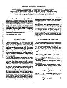
Ωx t FIG. 2. The evolution of the entanglement entropy (25) between the two modes for ky = 0.3kx > 0 and frequencies ω/ωy = 0.5 (A1 ), 0.95 (A2p ), 1 (A-D), 1.05 (D1 ), 1.7 (D2 ) and 1.95 (B), where ωµ = kµ and the label indicates the corresponding sector in Fig. 1. S(t) is quasiperiodic in curves A1 , A2 and B, but increases logarithmically (on average) in A-D, and linearly in D1 , D2 . The initial state is the separable ground state of H0 (uncoupled oscillators).

tion of f (t) and S(t) will be quasiperiodic, as seen in Fig. 2 (curves A1 , A2 and B). The initial state was chosen p as the ground state of h0 (αµ = kµ in (28)). Starting from point 1 in sector A (Fig. 1), the generated entanglement S(t) remains small p when ω is well below the first ky (curve A1 ). As ω increases, critical value ωy = S(t) will exhibit increasingly higher maxima, showing a typical resonant behavior for ω close to ωy (border with sector D), where λ− vanishes. Near this border, S(t) will essentially exhibit large amplitude low frequency oscillamπ tions determined by λ− , with maxima at t ≈ tm = 2λ − (m odd), plus low amplitude high frequency oscillations determined by λ+ , as seen in curve A2 . As ω increases, the system enters √ dynamically unstable sectors for ωy ≤ ω ≤ ωx = kx , and the evolution becomes unbounded (curves A-D, D1 and D2 , described in next subsection). For ω > ωx , the system reenters the dynamically stable regime and exhibits again the previous behaviors, with an oscillatory resonant type evolution for ω above but close to ωx (curve B in Fig. 2). Close to instability but still within the stable regime, the maximum entanglement reached is of order ln |ω − ωµ |: For ω close to ωµ (µ = x, y) on the stable side, and for the initial conditions (28), f (t) will be maximum at t ≈ tm , with r 2 f (tm ) ≈

ω|ε− | λ2+ λ−

where λ+ ≈

(

αx αy +ω λ+

)2 sin2

mπλ+ 2λ−

+α2µ cos2

αx αy

mπλ+ 2λ−

, (32)

q 2(ε+ + ωµ2 ) and λ− ≈

s

2ωµ |ε− ||ωµ − ω| , ε+ + ωµ2

(33)

6

4

2

a

S

3

S

8

b 4

1 0 0

0.5

1

k y kx

0 0

0.5

1

1.5

ِΩx 4

a

2

b

S

3

FIG. 4. The entanglement entropy between the two modes attained at fixed time ωx t = 40, as a function of the (constant) frequency ω, for the oscillator parameters and initial state of Fig. 2. Entanglement is bounded for ω < ωy (sector A) and ω > ωx (sector B), but is proportional to t in the instability window ωy < ω < ωx (sector D).

1 0 0

0.5

1

C.

Evolution in unstable sectors

k y kx FIG. 3. The maximum entanglement S(tm ) reached in stable sectors close to instability, as a function of the anisotropy ratio ky /kx (see Eq. (32)). Top: Vicinity of border A-D (ω = 0.999ωy ). Bottom: Vicinity of border B-D (ω = 1.001ωx ). The initial state is the separable ground state of H0 (αµ = ωµ ) in curves a and a separable isotropic state (αµ = 1) in curves b.

Let us now examine in detail the evolution of S(t) in the dynamically unstable regimes. At the critical frequencies ω = ωµ , µ = y, x (borders A-D and B-D), λ− vanishes and Eqs. (12) and (24) lead, for large t and the initial conditions (28), to the critical evolution r 2 −| f (t) ≈ t ω|ε λ2 +

where λ+ =

(

αx αy +ω λ+

)2 sin2 λ+ t+α2µ cos2 λ+ t αx αy

,

(34)

q 2(ε+ + ωµ2 ) > 0. This entails a linear

implying f (tm ) = O(|ωµ − ω|−1/2 ) and hence S(tm ) = O(− 12 ln |ωµ − ω|).

increase, on average, of f (t) in this limit, and hence, a logarithmic growth of S(t), according to Eq. (26):

Expression (32) (and hence S(tm )) will tend to decrease for decreasing anisotropy, i.e., increasing ratio ky /kx ≤ 1, as seen in Fig. 3 for m = 1, vanishing in the isotropic limit ky /kx → 1 (where f (tm ) = O(|kx − ky |)1/2 ). On the other hand, the behavior for ky /kx → 0 will depend on the initial condition: If it is the ground state of H0 (αµ = ωµ , curves a), f (tm ) will vanish at the √ first border ω ≈ ωy (top panel), where f (tm ) = O( ωy ), but diverge at the second border ω = ωx (bottom panel), √ where f (tm ) = O(1/ ωy ), as obtained from Eq. (32). If the initial state is fixed, however, f (tm ) will approach a finite value for ky /kx → 0, and exhibit a monotonous decrease on average with increasing ratio ky /kx in both borders (curves b in Fig. 3), as also implied by (32). We also mention that the high frequency oscillations in f (tm ) and S(tm ) observed in Fig. 3 stem from the λ+ /λ− ratio in the arguments of the trigonometric functions in Eq. (32). For ω close to ωµ , this ratio is minimum around ky /kx ≈ 1/5, which leads to the observed decrease in the oscillation frequency of S(tm ) in the vicinity of this ratio (top panel).

S(t) ≈ S0 (t) + ln t ,

(35)

where S0 (t) = 1 + ln[f (t)/t] is a bounded function oscillating with frequency λ+ . This behavior (curve A-D in Fig. 2) is the ω → ωµ limit of the previous resonant regime. On the other hand, in the unstable sector D (ωy < ω < ωx ), λ− becomes imaginary. This leads to an exponential − |t term in f (t) ( sinλλ−− t → sinh|λ|λ ), which will dominate −| the large t evolution: In this sector Eqs. (12), (24) and (27) imply, for large t, f (t) ∝ e|λ− |t , S(t) ≈ |λ− |t ,

(36)

and hence, a linear growth (on average) of the entanglement entropy with time (curves D1 , D2 in Fig. 2). Therefore, in the unstable window ωy ≤ ω ≤ ωx , there is an unbounded growth with time of the entanglement entropy, which will originate a pronounced maximum in the generated entanglement at a given fixed time and anisotropy as a function of ω, as appreciated in Fig. 4.

7

20

S2 + 4 ln t

3

S1 + 2 ln t

10

S

S

b

50

a

1

S0 HtL + ln t 0 0

2

0 0

100

30

Ωx t

We now examine the behavior at the other sectors of Fig. 1. In the unstable sectors C and E, where one or both of the constants kµ are negative, λ± are imaginary or complex (Fig. I). This implies an exponential increase of f (t), as indicated in table I, entailing again a linear asymptotic growth of the entanglement entropy with time: S(t) ≈ (|λ+ | + |λ− |)t in C and S(t) ≈ 2|Im(λ± )|t in E, neglecting constant or bounded terms. On the other hand, at the border between sectors B and E, which corresponds to the critical curve ∆ = 0 between both points L in Fig. 1, we obtain, for large t and kx 6= ky (with the initial conditions (28)), the asymptotic behavior 4ω 2 αx αy + ε2− 2 t , √ 16ωλ αx αy

p where λ = ε+ + ω 2 > 0. This leads to S(t) ≈ S1 + 2 ln t ,

,

FIG. 6. Evolution of the entanglement entropy for a stepwise varying frequency ω, starting from the separable ground state of H0 (with ky = 0.5kx > 0). In curve a we have set ω/ωx = 0.5, 0.7, 0 and 0.21 for successive time intervals of length ωx ∆t = 30, such that the system is close to the first instability p at the second interval (0.7ωx ≈ 0.99ωy , with ωµ = kµ ), while in curve b the only change is ω = 0.75ωx ≈ 1.06ωy in the second interval, such that the system enters there the unstable regime leading to a linear entanglement growth. This plot shows that entanglement can be increased, kept constant and returned to a vanishing value just by tuning the frequency ω.

implying the following logarithmic increase of S(t): S(t) ≈ S2 + 4 ln t ,

(40)

α α +ω 2

where S2 ≈ 1+ln[ 6x√αyx αy ω 3 ]. Hence, the increase is here still more rapid than at both previous borders. These critical behaviors are all depicted in Fig. 5.

D.

(38)

4ω 2 α α +ε2

αx αy +ω 2 3 4 √ 6 αx αy ω t

120

Entanglement control

(37)

with S1 ≈ 1 + ln[|ε− | 16ωλx√αy x αy− ]. Hence, the unbounded growth of f (t) and S(t) is here more rapid than that at the previous borders A-D and B-D (ω = ωy or ωx ) (quadratic instead of linear increase of f (t)). At the border E-C the asymptotic behavior of f (t) is still exponential (i.e., linear growth of S(t)). Finally, a further remarkable critical behavior arises at the special critical points L, obtained for condition (20), where all sectors B, C, D and E meet. We obtain here a purely polynomial evolution of (f (t) + 1/2)2 , as implied by Eqs. (21). For large t, this leads to a quartic increase of f (t): f (t) ≈

90

Ωx t

FIG. 5. Critical evolution of the entanglement entropy at the border between sectors with distinct dynamics, for isotropic initial conditions (αµ = 1). The lower, middle and upper curve correspondp respectively to the border A-D (at ky = 0.5kx , with ω = ky ), B-E (at ky = −1.5kx , with ω given by (18)) and the critical points L (Eq. (20)). The asymptotic behavior for large t (Eqs. (35), (38), (40)) is indicated.

f (t) ≈ |ε− |

60

(39)

We finally show in Fig. 6 the possibilities offered by this model for controlling the entanglement growth through a stepwise time dependent frequency, starting from the separable ground state of H0 . After applying a “low” initial frequency ω = 0.5ωx for ωx t < 30, which leads to a weak quasiperiodic entanglement, by p tuning ω to a value close to the first instability ωy = ky for a finite time (30 < ωx t < 60), it is possible to achieve a large entanglement increase (curve a). Then, by setting ω = 0 (i.e., switching off the field or rotation), entanglement is kept high and constant, since the evolution operator becomes a product of local mode evolutions. Finally, by turning the frequency on again up to a low value, entanglement can be made to exhibit strong oscillations, practically vanishing at the minimum if ω is appropriately tuned. Thus, disentanglement at specific times can be achieved if desired. The entanglement increase at the second interval can be enhanced by allowing the system to enter the instability region for a short time, as shown in curve b.

8

f,Xlz \

5

Xlz \ f

0 -5 0

30

60

90

120

Ωx t FIG. 7. Evolution of the average occupation number f (t) (Eq. (24)) and angular momentum hlz i for case a of Fig. 6.

The growth of the average occupation f (t) (and hence the entanglement entropy S(t)) in the second interval is strongly correlated with that of the average angular momentum hlz it , i.e., with the entangling term in H, as seen in Fig. 7 for case a of Fig. 6. Nonetheless, while the evolution of f (t) is similar to S(t), the average angular momentum exhibits pronounced oscillations when ω is switched off, since lz is not preserved in the present anisotropic trap ([lz , h0 ] 6= 0). These oscillations persist in the last interval, although shifted and partly attenuated. Here the vanishing of hlz it provides a check for the vanishing entanglement, since in a separable state hlz i = hqx ihpy i − hqy ihpx i and for the present initial conditions hqµ i = hpµ i = 0 for all times. Thus, f (t) = 0 implies here hlz it = 0, although the converse is not valid. Though initially correlated, we remark that hlz it and the average occupation f (t) do not have a fixed asymptotic relation in the whole plane. For instance, at the stability borders ω = ωµ , hlz it increases on average as t2 for high t, i.e., as f 2 (t) (Eq. (34)), and the same relation with f (t) holds in the unstable sector D (ωy < ω < ωx ), where hlz it ∝ e2|λ− |t . Nonetheless, in an unstable potential at the critical curve ∆ = 0, hlz it ∝ t2 (on average) for large t, increasing then as f (t) (Eq. (37)), while at the critical points L we obtain hlz it ∝ t6 , i.e., hlz it ∝ f 3/2 (t) asymptotically (Eq. (39)). IV.

CONCLUSIONS

We have analyzed the entanglement generated by an angular momentum coupling between two harmonic modes, when starting from a separable gaussian state. The general treatment considered here is fully analytic and valid throughout the entire parameter space, including stable and unstable regimes, as well as critical regimes where the system cannot be written in terms of normal coordinates or independent quadratic systems (non-diagonalizable H2 ). Hence, in spite of its simplicity, the present model is able to exhibit different types of en-

tanglement evolution, including quasiperiodic evolution, linear growth, and also logarithmic growth of the entanglement entropy with time, which can all be reached just by tuning the frequency. The model is then able to mimic the typical evolution regimes of the entanglement entropy encountered in more complex many-body systems. Even distinct types of critical logarithmic growth can be reached when allowing for general quadratic potentials. The system offers then the possibility of an easily controllable entanglement generation and growth, through stepwise frequency changes, which can also be tuned in order to disentangle the system at specific times. The model can therefore be of interest for continuous variable based quantum information. The authors acknowledge support from CONICET (LR,NC) and CIC (RR) of Argentina. We also thank Prof. S. Mandal for motivating discussions during his visit to our institute. A.

Appendix

In order to highlight the non-trivial character of the present model when considered for all real values of the constants kµ and frequency ω > 0, we provide here some further details [20]. With the sole exception of the critical curve ∆ = 0 (Eq. (18)), the Hamiltonian (3) can be written as a sum of two quadratic Hamiltonians, h=

1 1 2 2 (α+ p2+ + β+ q+ ) + (α− p2− + β− q− ), 2 2

(41)

where p± , q± are related with qx,y , px,y by the linear canonical transformation q

−ηp

y,x p± = px,y + γqy,x , q± = x,y (1+γη) , γ = (∆ − ε− )/(2ω) , η = γ/ε+ ,

(42)

such that [qr , ps ] = iδrs , [qr , qs ] = [pr , ps ] = 0 for r, s = ±, and α± =

1 ε− ± 2ω 2 + , 2 2∆

β± =

∆ (∆α± − ε− ) , ω2

with α± β± = λ2± (Eq. (10)). Nonetheless, the coefficients α± , β± can be positive, negative or zero, and may become even complex, according to the values of kx , ky and ω. We may obviously interchange p± with q± in (42) by a trivial canonical transformation p± → q± , q± → −p± . This freedom in the final form will be used in the following discussion. In sector A of Fig. 1, α± , β± in Eq. (41) are both real and positive, and the system is equivalent to two harmonic modes. Here λ± are both real. In sector B, α+ , β+ are positive but α− , β− are both negative, so that the system is here equivalent to a standard plus an “inverted” oscillator. Nevertheless, λ± remain still real. In sector C, α± β± < 0, and the effective quadratic potential becomes unstable in both coordinates (i.e., α± > 0, β± < 0). Here λ± are both imaginary. In sector D, α+

9 and β+ are positive but α− β− < 0, so that the potential is stable in one direction but unstable in the other (i.e., α− > 0, β− < 0). Here λ+ is real but λ− is imaginary. In sector E, both α± and β± are complex and q± , p± are non hermitian [20]. Here λ± are complex conjugates. At the border A-D, α+ , β+ , α− are all positive but β− = 0 (or similar with β− ↔ α− ), so that the system is equivalent to a harmonic oscillator plus a free particle (λ+ > 0, λ− = 0). The same holds at the border B-D, except that α− < 0 (inverted free particle term). At the Landau point F (kx = ky = ω 2 , where A, B, and D meet), α+ > 0, β+ > 0 but α− = β− = 0. Finally, at the border C-D, α+ > 0, β+ = 0 (or similar with β+ ↔ α+ ) and α− β− < 0, implying λ+ = 0 and λ− imaginary.

The decomposition (41) no longer holds at the critical curve ∆ = 0, which separates sector E from sectors C and D. At this curve (including points L), the system is inseparable, in the sense that it cannot be written as a sum of two independent quadratic systems, even if allowing for complex coordinates and momenta as in sector E. While the matrix H2 (Eq. (9)) is always diagonalizable for ∆ 6= 0, i.e., whenever the decomposition (41) is feasible, both H and H2 are non-diagonalizable when ∆ = 0. Here λ± = λ, with λ real at the border between B and E, imaginary between C and E and zero at the points L. The optimum decomposition of h in these cases is discussed in [20].

[1] J. Schachenmayer, B.P. Lanyon, C.F. Roos, A.J. Daley, Phys. Rev. X 3 031015 (2013). [2] J.H. Bardarson, F. Pollmann, J.E. Moore, Phys. Rev. Lett. 109 017202 (2012). [3] A.J. Daley, H. Pichler, J. Schachenmayer, P. Zoller, Phys. Rev. Lett. 109 020505 (2012). [4] C.H. Bennett et al., Phys. Rev. Lett. 70, 1895 (1993); Phys. Rev. Lett. 76, 722 (1996). [5] M.A. Nielsen and I.L. Chuang, Quantum Computation and Quantum Information (Cambridge Univ. Press, Cambridge, UK, 2000). [6] R. Josza and N. Linden, Proc. R. Soc. A 459, 2011 (2003). [7] G. Vidal, Phys. Rev. Lett. 91, 147902 (2003). [8] N. Schuch, M. M.Wolf, F. Verstraete, and J. I. Cirac, Phys. Rev. Lett. 100, 030504 (2008). [9] J.G. Valatin, Proc. R. Soc. London 238, 132 (1956). [10] A. Feldman and A. H. Kahn, Phys. Rev. B 1, 4584 (1970). [11] P. Ring and P. Schuck, The Nuclear Many-Body Problem, (Springer, NY, 1980). [12] J.P. Blaizot and G. Ripka, Quantum Theory of Finite Systems (MIT Press, MA, 1986). [13] A.V. Madhav, T. Chakraborty, Phys. Rev. B 49, 8163 (1994). [14] M. Linn, M. Niemeyer, and A. L. Fetter, Phys. Rev. A 64, 023602 (2001). ¨ Oktel, Phys. Rev. A 69, 023618 (2004). [15] M. O. [16] A. L. Fetter, Phys. Rev. A 75, 013620 (2007). [17] A. Aftalion, X. Blanc, and N. Lerner, Phys. Rev. A 79, 011603(R) (2009). [18] A. Aftalion, X. Blanc, J. Dalibard, Phys. Rev. A 71, 023611 (2005); S. Stock et al, Laser Phys. Lett. 2, 275 (2005). [19] A.L. Fetter, Rev. Mod. Phys. 81, 647 (2009). I. Bloch, J. Dalibard, W. Zwerger, Rev. Mod. Phys. 80, 885 (2008); [20] R. Rossignoli and A.M. Kowalski, Phys. Rev. A 79

062103 (2009). [21] R.F. Werner, M.M. Wolf, Phys. Rev. Lett. 86, 3658 (2001). [22] K. Audenaert, J. Eisert, M.B. Plenio, and R.F. Werner, Phys. Rev. A 66, 042327 (2002). [23] G. Adesso, A. Serafini, and F. Illuminati, Phys. Rev. A 70, 022318 (2004); A. Serafini, G. Adesso, and F. Illuminati, Phys. Rev. A 71, 032349 (2005). [24] S.L. Braunstein and P. van Loock, Rev. Mod. Phys. 77, 513 (2005). [25] C. Weedbrook et al, Rev. Mod. Phys. 84, 621. [26] J. Pˇerina, Z. Hradil, and B. Jurˇco, Quantum optics and Fundamentals of Physics (Kluwer, Dordrecht, 1994); N. Korolkova, J. Pˇerina, Opt. Comm. 136, 135 (1996). [27] L. Reb´ on, R. Rossignoli, Phys. Rev. A 84, 052320 (2011). [28] A.P. Hines, R. H. McKenzie, and G.J. Milburn, Phys. Rev. A 67, 013609 (2003). [29] H.T. Ng, P.T. Leung, Phys. Rev. A 71, 013601 (2005). [30] A.V. Chizhov, R.G. Nazmitdinov, Phys. Rev. A 78, 064302 (2008). [31] V. Sudhir, M.G. Genoni, J. Lee, M.S. Kim, Phys. Rev. A 86, 012316 (2012). [32] R. Rossignoli and C.T. Schmiegelow, Phys. Rev. A 75, 012320 (2007). [33] L. Amico, et al, Phys. Rev. A bf 69, 022304 (2004); A. Sen(De), U. Sen, and M. Lewenstein, Phys. Rev. A 70, 060304(R) (2004); 72, 052319 (2005). [34] S.D. Hamieh and M.I. Katsnelson, Phys. Rev. A 72, 032316 (2005); Z. Huang, S. Kais, Phys. Rev. A 73, 022339 (2006); M. Koniorczyk, P. Rapcan, V. Buzek, Phys. Rev. A 72, 022321 (2005). [35] L. Amico, R. Fazio, A. Osterloh and V. Vedral, Rev. Mod. Phys. 80, 516 (2008). [36] A.K. Ekert et al, Phys. Rev. Let.. 88, 217901 (2002); C.M. Alves, D. Jaksch, Phys. Rev. Let.. 93, 110501 (2004).