Dynamics of finite causal processes

Earth Syst. Dynam. Discuss., https://doi.org/10.5194/esd-2018-20 Manuscript under review for journal Earth Syst. Dynam. Discussion started: 2 May 2018 c Author(s) 2018. CC BY 4.0 License.

Dynamics of finite causal processes Kalman Ziha University of Zagreb, Faculty of Mechanical Engineering and Naval Architecture, 10002 Zagreb, Ivana Lucica 5, Croatia Correspondence to: Kalman Ziha ([email protected]) 5

Abstract. Earth and environmental mechanisms and phenomena are often physically finite dynamical causal processes and need more precise mathematical elaboration. Therefore this article at the beginning resumes the decomposition of general infinite circular causal relations with linear feedbacks to primary causal effects and to interactions among boundless effects and causes. In the sequel it reveals the mathematical model of general finite cause-and-effect interaction with non-linear feedback induced by finiteness of causal processes with exhaustible causal capacities. The study also uncovers that the reverse

10

application of the mathematical model makes it possible to discover and to estimate the unknown ultimate causal capacities from relevant information of supposedly finite causal processes beyond the instant of observation. The article at the end demonstrates that the environmental relations among global climate change and ice mass losses monitored recently on Greenland and Antarctica ice sheets are plausibly finite dynamical climate processes in interaction with cryosphere.

1 Introduction 15

This study aims to find out if there are synthetic measurable theoretically founded quantitative parameters of a general mathematical model appropriate for analysis and predictions of complex interactions of natural finite causal processes. The mathematical model of finite dynamical causal processes in the article follows the concepts of quantitative theory of growth (von Bertalanffy, 1938), control systems (Wiener, 1948) and open systems in general system theory (von Bertalanffy, 1968). Natural Cause-and-Effect relations (CE) and Circular Causation interrelations (CC) of interacting Effects (E) and Causes (C)

20

are in reality often limited by available ultimate normally exhaustible and finite causal capacities CU. The empirical problem of interactions of limited causal processes is tackled in the study by a general mathematical model of Finite Cause-and-Effect Interaction (FCEI) concept. The guiding thought is that complex interactions of finite natural causal processes and limited environmental resources under multifarious conditions implying feedbacks (F) and interactions (I) can be mathematically decomposed into simple CE and to finite FCEI relations. The study embraces that the mere existence of finiteness of causal

25

processes itself induces non-linear feedbacks F[E(C)] of effects E(C) of causes C in the FCEI processes. These feedbacks are the results solely of the fact that there are real limited residual driving causes R=CU-C after some cause C elapsed on the expense of the ultimate causal capacity CU. The finite interaction I(E,C) between the effect E and the cause C is regarded in this study as the forthcoming effect of the feedback F[E(C)] to effect E(C) induced only by the finite causal capacity CU. Accordingly, the FCEI concept may be applied in reverse direction in discovery and estimation of unknown ultimate capacity 1


CU from past partial data of supposedly finite causal processes in the future. The FCEI concept basically represent the physical interchanging processes of physical entities among elapsed effects and forthcoming residual causes beyond the moments of direct observations. The concept was tested earlier on problems of fatigue yielding (Ziha 2009), general considerations on how things worsen (Ziha 2012), ageing and fatigue (Ziha 2014), material plasticity (Ziha, 2015) and fatigue life predictions in 5

engineering (Ziha 2016). The study investigates and demonstrates the appropriateness of the mathematical model of Finite ice Melting (the cause M) and ice mass Losses (the effect L) Interaction (FMLI) on the numerical analysis of the interaction of climate changes and the recently observed alarming land ice mass anomaly of Greenland and Antarctica ice sheets (Velicogna and Wahr, 2006a; Velicogna and Wahr, 2006b; Velicogna, 2009; Sasgen et al., 2013; Velicogna et al., 2014;; Tedesco et al., 2015; Tedesco et al., 2016; Tedesco et al. 2017; Wiese et al., 2016).

10

2 Concept of general cause and effect interaction Traditional readings on causation in terms of invariable patterns of succession lead to regularity theories which imply that the cause C and the effect E are connected but different entities. That C affects E is the singular causal claim CE where C and E are relata of the claim. The prevailing present comprehension of causality is that the knowledge of causal relations arises entirely from experience. The conclusions made from experience imply a belief that some observable courses of nature could

15

be sufficiently uniform so that the future would be conformable to the past. There is no assertion with respect to directionality of causation, except for the common experience that an effect does not influence in reverse the cause C  E (asymmetry). It is commonly agreed that the flow of causality proceeds from past to the present into the future which are unavoidably separated by the inherent human ability of perceiving only at the instant of observation. Such a belief makes possible the prediction of the course of progress of a CE relation beyond the moment of observation unnefected by the future. In physical

20

view of causal determinism the world-at-a-time has an objective notion in which the particular causes C and effects E(C) of C are normally regarded as empirical laws of nature. The claim, according to which every later effect is uniquely determined by its earlier cause, doesn’t necessarily regards interactions of E and C. 2.1 The simple infinite cause and effect mathematical relation The simple CE relation of a causal model where the unaffected primary cause is directly linearly applied to the primary effect

25

E’(C) in proportion p that represents the CE progression factor, can be mathematically presented as:

E '(C )  p  C

(1)

An infinite causal relation is theoretically not limited in its progression and may unaffectedly continue beyond the instant of observation following the empirical causal term in (1). The rate of change of the primary infinite causal relation (1) in which the ultimate causal capacity CU is undefined, i.e. considered infinite, is simply constant: 30

dE '(C ) / dC  E '(C ) / C  p

(2)

2


2.2 The infinite cause and effect interaction induced by feedback The general infinite CE relation in (1) and (2) is the linear CE relation representing an open loop system in system dynamics where the parameter p is denoted as the open-loop gain. However, the general CE relation (1) in open and active environment can ensue as a continuous relation in which the elapsed effect E’(C) induced by the primary cause C at the instant of observation 5

has been influencing the forthcoming secondary cause C’’ (Wiener, 1948; von Bertalanffy 1968). The fraction f of the primary effect E’(C) in (3) may turn to feedback F affecting the primary cause C in the C-E space where f is denoted in the control theory as the feedback factor. The feedback F to primary effect E’(C) is defined as:

F  E '(C )   f  E '(C )  f  p  C

(3)

The definition of the secondary cause C’’{F[E’(C)]} induced by the feedback F[E’(C)] (3) to the primary effect E’(C) (1) (Fig. 10

1) which is affecting in turn the primary cause C is then defined as follows:

C ''  C  F  E '(C )   C  f  E '(C )  C  f  p  C  (1  i )  C

(4)

In (3) and (4) i=f p is the parameter combined of the feedback factor f in (3) and progression factor p in (1) that represents the intensity of interaction between the elapsed effect and the forthcoming cause. Substituting the value of the primary cause C from (4) into the primary effect (1) it follows 15

E '(C )  p  C '' F  E '(C ) . The primary effect E’(C) is after rearrangement expressed by the forthcoming cause C’’ (Fig. 1) as shown:

E '(C )  C '' p / (i  1)

(5)

Terms (3) and (4) represent the circular causality (CC) of interrelated sequence of interacting cause C and effect E with constant feedback F (3) that form a closed-loop system like a circuit or a loop. 20

2.3 The mathematical decomposition of the causal relation In some temporal circular causal (CC) systems the delivery of the feedback F in (3) may occur instantaneously or in a very short time unimportant for outcome of the CE relation for a conscious observer. The overall effect E(C) of the cause C at the perceptible moment of observation may be then taken as equal to the effect of the CE relation (1) up to the forthcoming effect C’’ induced by the feedback F, that is, E’(C’’)=p C’’ (Fig. 1). The overall effect E(C) at the moment of observation is

25

mathematically decomposable to the primary elapsed effect E’(C) as in (1) and to the effect of feedback E’{F[E’(C)]}=p F[E’(C)] as in (3) for the whole range of the cause C as shown:

E (C )  E '(C '')  p  C ''  (1  i )  E '(C )  E '(C )  E 'F  E '(C )   E '(C )  I ( E , C )

(6)

The effectiveness q of the circular causal relation with feedback (5) is denoted as the closed-loop gain and can be presented as

q  E '(C ) / C ''  E '(C ) / E (C ) / p  p / (1  i ) .

3


The temporal effect of feedback E’{F[E’(C)]} in (6) is defined in this study as the interaction I(E,C) at the moment of observation between the forthcoming cause C’’ in the future and the elapsed primary effect E’(C) in the past (Fig. 1). The interaction I(E,C) depending on the intensity i representing both the feedback factor f and the open-loop gain p, is then:

I ( E, C )  E 'F  E '(C )  p  F  E '(C )   E '  f  E '(C )   f  p  E '(C )  i  p  C 5

(7)

Note that the feedback in (3) is inversely related to the interaction (7) as {F[E’(C)]}= E’-1[I(E,C)]. The rate of change of the interaction term for constant feedback is simply constant obtained by chain derivative of (7):

dI ( E, C ) E 'F  E '(C ) dI ( E , C ) dF ( E , C ) dE '(C )      f  p2  i  p dC C dF ( E , C ) dE '(C ) dC

(8)

Note also that for E’(C)=C is p=1 in (1), and consequently, the interaction (7) is equal to the feedback (3), that is I(E,C)={F[E’(C)]}. The appropriate rate of change of the overall effect E(C) (6) with feedback (3) (Fig. 1) is 10

dE (C ) / dC  p  (1  i ) . The overall theoretical potential W of interaction I(E,C) (7) can be calculated by the integration of (7) up to the primary cause C at the instant of observation as follows: C

W  I ( E, C    I ( E, C ) d C  i  E '(C ) 2 / (2  p)  i  p  C 2 / 2

(9)

0

The interaction intensity parameter i in (7) and (8) can be calculated directly from the known interaction potential W (9): 15

i  2  p  W  I ( E , C )  / E '(C ) 2  2  W  I ( E , C )  / ( p  C 2 )

Figure 1: Decomposition of general cause-and-effect relation with linear feedback in the C-E space.

4

(10)


3 Finite cause and effect interaction This study of finiteness of natural processes recognises the temporal FCEI empirical concept as a continuous sharing of irreplaceable and restricted overall ultimate causal capacity CU between the observable elapsed effect E in the past and the imperceptible but conceivable forthcoming limited exhaustible cause C beyond the instant of observation in the future (Fig. 5

2). The trans-temporal finite interaction implies the empirical link in continuation of the known uninterrupted past and the imaginable but finite perpetuating future separated by the instant of observation at the present time. The finiteness affects causal processes solely by the fact that there is really a limited ultimate and final causal capacity CU (see Appendix A). The mathematical model of the FCEI in this study considers a simple intuitive term of the continuous residual causal capacity R(C) after spending some primary effect E’(C) (1) of the limited cause C on the expense of the ultimate cause CU. The leftover

10

driving cause R(C) for the future uninterrupted perpetuation of the CE relation is defined in a linear form as:

R(C )  (CU  C )  CU  (1  c)

(11)

In (11) c=C/CU is the relative linear progression of the elapsed cause C with respect to the ultimate causal capacity CU. 3.1. The feedback of finiteness to causal processes The following expression defines the mathematical rate of the finite interaction dIF(E,C) as the relation of the effect 15

E’{F[E’(C)]} of the feedback F[E’(C)] (3) of the elapsed effect E’(C) (1) and the remaining capacity (CU-C) (11) instead of the mere effect of the progressing linear cause C as it is in the general infinite interaction model (8) (Fig. 2) as shown: E ' F  E '(C )  dI F ( E , C ) dE '(C ) C dI ( E , C ) c    i p   dC R (C ) d(CU - C ) (CU  C ) dC 1 c

(12)

The accumulation of the forthcoming finite interactions depends on the remaining cause R(C) (11) rather than on the elapsed effect E’(C) as in (8) and can be calculated by integration of the differential equation of the variable rate of change (12) until 20

the primary cause C at the instant of observation (see Appendix A) as follows: C

I F (E, C )   0

C CU  dI F ( E , C ) dC  i  p  C  i  p   U  ln   C  i  p  u (c )  C  I ( E , C )  u (c ) dC CU  C   C

(13)

In (13) u(c) is the dimensionless finite interaction intensity correction function of the general interaction term (7) for limited causal capacity (11) of logarithmic shape and of asymptotic character depending only on the relative FCEI progression c as: u (c)  1 

25

1 1  ln c 1 c

(14)

The variable rate of sharing of the causal capacity C/(CU-C) at the moment of observation between the elapsed cause C in the past and the remaining cause (CU-C) (12) in the future characterizes the influence of the causal finiteness on the progression of the causal process. The overall effect E(C) is then a FCEI where the finite interaction IF(E,C) (13) analogously to the general interaction I(E,C) in (6) influences the primary effect E’(C) (1) (Fig. 2) as shown:

5


E (C )  E '(C )  I F ( E , C )  p  C  p  F  E '(C )   p  C  i  p  u (c)  C

(15)

The interaction rate (12) geometrically represents the continuously changing angles of tangents on the interaction curve (13) which determine the dynamics of the progression of the FCEI relation (Fig. 2). The effectiveness q of the circular causal relation with feedback (15) is denoted as the closed-loop gain q  E '(C ) / E (C ) / p  p / 1  i  u (c)  . 5

The ending cause CE of the ultimately attainable effect E(CE) (15) (Fig. 2) is the solution of the inverse of equation of overall effect (15) as shown:

CE  cE  CU  E 1  E '(C  CU ) 

(16)

The ending cause CE in (16) is not algebraically separable from (15). The overall finite interaction potential WF can be calculated by the integration of (13) (Fig. 2), as shown below: C

10

WF  I F ( E , C )    I F ( E , C )dC  CU  i  p  w(c )  C

(17)

0

In (17), w(c) is the dimensionless interaction potential function depending only on the relative progression c as follows:

w(c)  c / 2  u (c)  ln(1  c)

(18)

The interaction intensity parameter i can be calculated from the definition of the overall interaction potential WF (17) as:

i  WF  I F ( E , C ) /  p  CU  w(c)  C  15

(19)

The second derivative of the overall effect E(C) (15), i.e. the sensitivity of the interaction rate (12) is as follows:

d 2 E (C ) i 1   p 2 dC CU (1  c) 2

(20)

The mathematical definition of the derivatives of functions with respect to bounds of finite variables (Fig. 2) is given in Appendix A. The variable term F[E’(C)] for feedback is a direct consequence of the effect of finiteness. It is inversely related to the 20

interaction term (13) (Fig. 2) as F  E '(C )   E’1  I F  E , C    I F ( E , C ) / p  i  u (c)  C .   The secondary cause C’’{F[E’(C)]} (4) induced by the variable feedback F[E’(C)] to the primary effect E’(C) (Fig. 2) which is affecting the finite primary cause C is then as C ''  C  F  E '(C )   C  i  u (c)  C . The effectiveness of the FCEI relation (15) is q  E '(C ) / C ''  p / 1  i  u (c)  with respect to the closed-loop gain in (5). The separation of the cause C(E) from the nonlinear part of the FCEI (13) I N (C )  i  p  CU  ln CU / (CU  C )  corresponds to the

25

von Bertalanffy asymptotic growth function (von Bertalanffy, 1938) (VBGF) of the cause C in the form

C  I N (C )  CU  1  e k I N (C )  where k=1/(ipCU) and CU represents the ultimate growth of the cause C depending on the effect E.

6


Figure 2: Decomposition of finite cause and effect interaction in C-E space.

3.2. Numerical estimation of the ultimate causal capacity C U 5

The FCEI mathematical model (11-20) normally provides the interaction term IF (13), the overall effect E(C) (15), the rate of change dE/dC (12), the sensitivity d2E/dC2 (20), the theoretical interaction potential WF (17) and interaction intensity i (19) of finite processes for known ultimate causal capacity CU. The reverse FCEI mathematical procedure makes it possible to estimate the unknown ultimate causal capacity CU and the interaction intensity i from the past data of supposedly finite causal processes even beyond the instant of observation.

10 The numerical solution of this task can be defined for example as a general non-linear optimization program as shown: FCEI-OPP: Optimization program for estimation of ultimate causal capacity CU and intensity i from observed data:

15



Estimate E(Co), dE/dCo, and d2E/dCo2 (11-20) at the moment of observation (e.g. apt fitting to observed data (Fig. 2)).



Estimate interaction potential Wo (e.g. by numerical integration of observed data (Fig. 2)).



Set objectives WF(Co, CU, i)=Wo and d2E/dC2=d2E/dCo2 by changing CU and i in (17) as free variables. 7


4 Climate change and ice melting interaction Decades of researches of climate dynamics and climatic change relating cryosphere have been highlighting many complex hardly jointly manageable interrelated causes and effects as well as the importance of a number of various feedbacks and interactions of the land ice sheets, the sea ice, the sea level elevation, atmosphere, hydrosphere, oceans and the global climate 5

system. The meanings of multiple feedback mechanisms and interactions giving rise to the aperiodic oscillations in climate systems including ice-albedo feedback, precipitation-temperature feedback and interactions between the ice sheets and the bedrock has been earlier identified in investigation of climatic change (Yiou et al., 1994). The study of the Greenland surface ice mass balance confirmed the significance of the feedback between the surface climate and the surface albedo in energybalance-based ablation calculations of interest for climate dynamics (Lefebre et al., 2005). Different interactions and feedbacks

10

of long-term ice sheet-climate and anthropogenic climate change were studied in order to investigate the sea level rise and the impact of ice sheet changes on the climate system (Vizcaino et al., 2008). Ice-climate interactions and climate sensitivity were also investigated by considering the Greenland and Antarctica ice sheet climate dynamics (Goelzer et al., 2011). The relevance of atmosphere and ice sheet interaction is recognized for study of ice sheet stability and ice mass balance formulation (Solgaard and Langen, 2012). The interactions of land ice sheets and climate has a long history and it is investigated on long time scale

15

accounting for ice-albedo and surface elevation feedback also accounting for the influence of CO2 and insolation by transient simulation of the past 800000 years (Stap et al., 2014). Moreover, researchers take for granted that the interaction between the climate system and the large polar ice sheet regions is a key process in global environmental change regarding the cryosphere (Gong, Cornford and Payne, 2014). The GRACE (Gravity Recovery and Climate Experiment) time-variable gravity satellite observations on a monthly basis from

20

April 2002 to June 2017 (Velicogna and Wahr, 2006a; Velicogna and Wahr, 2006b; Velicogna, 2009; Sasgen et al., 2013; Velicogna et al., 2014; Tedesco et al., 2015; Tedesco et al., 2016; Tedesco et al., 2017; Wiese et al., 2016) indicated supralinear growth of annual average rates of ice mass losses in the period of Ts=152/12 years of about 286 Gt/year for the Greenland ice sheet and 127 Gt/year for the Antarctica ice sheet, respectively (for example Figs. 3 and 4). For all these reasons this study aims to investigate whether the general concept of finite causal processes formulated by the

25

FCEI mathematical model (11-20) in this article can confirm the relation of the climate change feedback F and interaction I between ice malting M (the cause C) and ice mass losses L(M) (the effect E) as finite dynamical causal process (FMLI). 4.1 Finite ice melting and ice mass losses mathematical model The primary ice mass losses L’[M(T) in time T are related of the primary ice melting M(T) according to (1) as it is shown:

L '  M (T )   M (T )  t  T 30

(21)

The rate t=L/T in Gt/year of primary ice mass loss L during observation time T at the beginning of systematic data collection indicates the initial propensity to ice mass losses L[M(T) during ice melting M(T) (Figs. 3 and 4) in T-L and M-M-L spaces.

8


The remaining ice mass R(M) after an observed mass M of ice has melted out of the total finite mass MU of ice sheets is defined following (11) as shown

R( M )  MU  M  MU  (1  m)

(22)

In (22) m=M/MU=tT/MU is the observed ice melting M relative to the supposed ultimate mass MU of ice sheets. 5

4.2 Interaction of environmental thermal energy and ice sheet heat capacity The reported acceleration of ice mass losses alarmed that an increasing amount of environmental heat H[M(T)] of the climate system has been transferring to the melting mass M of ice sheets during the observation time T. Simultaneously the ice sheets during this heat transfer have been losing their total inherent finite heat capacity Q(MU). The reduction of the heat capacity Q[M(T)] (e.g. in GJ) of the ice sheets may be considered in proportion h to the mass of melted ice M in time T as shown:

10

Q  M (T )   h  M (T )

(23)

In (23) h is the specific heat capacity of ice at some temperature K (e.g. 2.108 x 103 (GJ/(Gt K) or particularly the specific latent heat of fusion h (e.g. 3.34 x 108 GJ/Gt) during transition from solid state of ice to liquid state. The diminishing residual heat capacity Q[MU-M(T)] after the mass M of ice has melted in time T is proportional to the remaining ice mass of the ice sheets MU-M (22) as shown: 15

Q  M U  M (T )   h   M U  M (T ) 

(24)

The character of the reported ice mass anomaly suggests that the heat flow from the environmental thermal energy plausibly intensifies at least linearly in proportion i to the loss of the heat capacity Q[M(T)] (23) of ice sheets as shown:

H  M (T )   i  h  M (T )

(25)

The parameter i in (25) represents the heat transfer interaction intensity between the environmental heat energy of the 20

climate system and the heat capacity of ice sheets. 4.3 Finite interaction of ice melting and ice losses The rate of the heat transfer from the environmental climate system to the ice sheets is defined according to (12) as the ratio of the increasing thermal energy H[M(T)] (25) of the environmental climate system and the diminishing residual heat capacity Q[MU-M(T)] (24) of the ice sheets as follows:

25

dI F  L, M (T ) dT



H  M (T )

Q  M U  M (T )

 i

m t 1 m

(26)

The last term (26) expresses the interaction between the climate system heating and the melting of ice sheets exactly in the same form of the FCEI interaction rate as in (12) but now expressed by relation of melted M and remaining MU-M (22) ice masses. The term (26) expresses the physical rate of heat energy flow from the climate system to the ice sheets in term of the melted ice mass and thermal energy equivalencies (23-25) (Figs. 3 and 4). 9


Hence, the study applies in the sequel the FCEI mathematical model (11-20) with the aim to investigate whether the relations of climate change and ice mass losses of ice sheets may be considered as finite dynamical causal processes. The integration of (26) yields to the FMLI interaction term as in (13) where the non-dimensional function u(m) (14) represents the effect of the ultimate ice mass MU to ice melting M in T-L space o in M-L space (Figs. 3 and 4) as follows: 5

I F  L, M (T )  

M

i M 0

M (T ) dM  i  u (m)  M  i  u (m)  t  T U  M (T )

(27)

The overall ice mass loss L[M(T) yields to the FMLI relation following (15) as shown: L  M (T )   L '  M (T )   I F  L, M (T )   1  i  u (m)   t  T

(28)

The theoretical finite interaction potential WF[IF(L,M(T)) during ice melting M exposed to climate conditions is expressed by the integral of (27) where w(m) is given in (17), respectively, as shown: 10

WF  I F ( L, M (T )  

T

 I  L, M (T )  dM F

 M U  i  w(m)  T

(29)

0

The overall theoretical finite potential during ice melting M exposed to climate conditions implies the potential of primary ice melting (21) and interaction potential (29) as shown:

W  L, M (T )  

T

 L  M (T )  dM

 M U   m / 2  i  w(m)   T

(30)

0

The theoretical total finite potential W[L, M(T)] (30) represents the mass equivalence (e.g. in Gt x year) to the overall 15

accumulated real work done by all environmental effects, that is, the absorbed external thermal energy H[M(T)] (25) of all sources of the climate system on expense of the loss of the diminishing heat capacity Q[M(T)] (23) during the melting of mas M of the ice sheets in time T. Negative intensity interaction parameter i in (21-30) indicates possible recovery. The first derivative of the ice mass losses L[M(T) (28) is the rate of change of the interaction (27) of the FMLI as follows:

m  m    dL  M (T )  / dT   p  i     p  i   t 1 m  1 m    20

(31)

The second derivative of the ice mass losses L[M(T) (28) is the rate of change of the interaction (27), that is, the sensitivity of the FMLI as follows:

d 2 L  M (T )  / dT 2  dI F  L, M (T )  / dT 

i 1  t2 2 M U (1  m)

(32)

The time of the beginning of the intense ice mass anomaly TB before the start of observations at To follows from the condition of the minimal rate of ice mass losses dL/dT=0 in (28) and can be calculated as shown: 25

TB  To 

MU 1  t (i  1)

(33)

The total melting out time TM for the ultimate loss of the ice mass MU of ice sheets is the numerical solution of the inverse of the equation (28) TM  L1 (MU ) . The fracture of interaction potential with respect to total potential is simply WF/W. 10


The total potential to finite melting out for mM=(t TM)/MU in (30) and for full melting out time T=TM amounts to WM=MU [mM/2+i w(mM) TM. The ratio of WF (29) and W (30) indicates the relative importance of the interaction potential. The total mass MU of ice sheets and the interaction intensity i are determined by the optimization program FCEI-OPP by the following numerically procedure: 5



Estimate Mo, dL/dMo, d2L/dM2 and t at the start of observation To (e.g. appropriate fitting to observed data (Fig. 2)).



Estimate the total potential Wo of the process (30) (e.g. by numerical integration of observed data (Fig. 2)).



Apply FCEI-OPP: Fulfil the above equality



The interaction intensity is then i= MU d2L/dM2.

W  L, M o , M U   Wo by changing MU as a free variable.

The FMLI mathematical model (21-34) is applied in the sequel to investigate the interactions between the ice mass loss of the 10

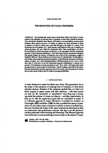
Greenland and Antarctica ice sheets and the climate change (Figs. 3 and 4). The following analysis gratefully uses the data from the GRACE JPL RL05M.1 Mascon Solution: Version 2 provided by Wiese et al. (2016).

Antarctica

MU=2.55 x 107 Gt t=dL/dT=42.25 Gt/year i=125784 d2L/dT2 =10.1 Gt/year2 W=10987 Gt x year WF=5794 Gt x year WF/W=0.53 TB=1997 year TM~4240 year

1996

Antarctica TB=1997 year Greenland TB=1964 year 1998

2000

2002

Observation period 2004

2006

2008

2010

Date years - T

2012

2014

2016

2018

2020

Antarctica MU=2.55 x 107 Gt i=125784 dL/dM=1 Gt/Gt d2L/dM2 =4.93 x 10-3 Gt/Gt2 W=497176 Gt x Gt M=685 Gt

Ice mass losses L Gt

MU=2.50 x 106 Gt t=dL/dT=232 Gt/year i=282.4 d2L/dT2 =6.08 Gt/year2 W=30150 Gt x year WF=3526 Gt x year WF/W=0.12 TB=1964 year TM~2800 year

Greenland MU=2.50 x 106 Gt i=282.4 dL/dM=1 Gt/Gt d2L/dM2 =1.13 x 10-4 Gt/Gt2 W=6995000 Gt x Gt M=3514 Gt

Antarctica -102 Gt

5000 4800 4600 4400 4200 4000 3800 3600 3400 3200 3000 2800 2600 2400 2200 2000 1800 1600 1400 1200 1000 800 600 400 200 0 -200 -400 -600

Greenland

Start of observations


5000 4800 4600 4400 4200 4000 3800 3600 3400 3200 3000 2800 2600 2400 2200 2000 1800 1600 1400 1200 1000 800 600 400 200 0 -200 -400 -600

-500.00

Greenland -988 Gt 0.00

500.00

Observation period 1000.00 1500.00 2000.00 2500.00 3000.00 3500.00 4000.00

Ice melting M Gt

Figure 3: Greenland and Antarctica reported ice mass anomaly analysis and FMLI numerical results in T-L and M-L spaces.

15

4.4 Interaction of ice melting and ice mass losses of the Greenland ice sheet.

Volume and mass of ice sheets are not precisely known. The density of glacier ice is estimated in the range of ice=0.900-0.917 Gt/km3. Greenland land ice sheet volume is estimated from different sources at VU=2.50-3.00 x 106 km3 and the total ice mass in the range MU= 2.50.20 x 106 Gt (8%). The Greenland sheet ice mass using a coherent ice-penetrating radar system to produce a thickness grid is estimated to 2.93 x 106 km3 or to about 2.65 x 106 Gt (Bamber et al., (2001). 20

A. The analysis of observed data by Wiese et al. (2016) provides the total external work done by all environmental effects, in terms of mass equivalence to the thermal energy of the climate system absorbed during 152/12 years of melting of the ice sheet that equals to the potential (30). It is estimated by numerical integration of observed data using the trapezium rule in amount of Wo[T=152/12 years)=30150.7 Gt x year in T-L space (30) or 6995000 Gt x Gt in M-L space (Fig. 3). 11


B. Preliminary fitting of the 2nd order parabola in T-L space L[M(T)=aT2+bT+c (Fig. 5) to the observed data that satisfies the above condition for total observed potential (30) Wo[T=152/12 years)= 30150.7 Gt x year provides a=3.04, b=232 and c=0.09. Fitting of the 2nd order parabola cannot provide information on ultimate mass MU of the ice sheet. C. For calculated total potential (30) W[T=152/12 years)=30150.7 Gt x year same as the observed potential Wo and for estimated acceleration d2L/dT2=2a=6.08 (Gt/year)/year (32), the optimization program FCEI-OPP provides the FMLI

5

interaction intensity parameter i=282.4 and the total ice mass of Greenland ice sheet of MU= 2.50 x 106 Gt (Fig. 3). This is a good estimate within the assumed range MU= 2.50.20 x 106 (8%) and with respect to 2.65 x 106 Gt (Bamber et al. (2001). The coefficient of determination R-squared between observed data and FMLI curve is R2=0.978. D. Final analysis by using the FMLI model provides additional information on Greenland ice mass melting. 10



The rates of ice mass loss L (31) in Greenland increased from dL/dT~230 Gt/year in 2002 to ~275 Gt/year in 2009 and to ~325 Gt/year at the end of observation in 2017 confirming the nonlinear character of the ice mass loss (Fig. 3) at an average of ~4133/152/12 =280 Gt/year or about 23 Gt/month during the observation period. Reported average is 286 Gt/year, Wiese et al. 2016).



The alarming acceleration of ice mass loss rates (32) starts at the beginning of the observations in the amount of d2L/dT2=6.08 (Gt/year)/year and slightly increasing in the future. The total observed ice mass loss is 4212 Gt.

15 

The interaction part (29) of the total potential (30) of the climate system and the ice melting is calculated in amount of WF[T=152/12 years)=3526 Gt x year (29), that is about 12% of the total potential (above the primary losses line Fig. 3).



By extrapolating the FMLI curve (28) to the past time, the estimated beginning of the intensive ice mass anomaly on Greenland relative to the start of observations at the date TB=20024/12 – 384/12 ~1964 (33), (Fig. 3).

20



Since the beginning of intensive losses to the start of observation on Greenland during 384/12 years about 988 Gt of ice have been already lost. To the end of observation during 38 4/12+152/12=5310/12 years about 988+4212=5200 Gt of ice is lost, what is 0.2% of the total ice mass MU (Fig. 3).



It is possible to predict by extrapolating the FMLI ice mass loss curve (28) that the melting out of the total mass of ice MU= 2.50 x 106 Gt due to the interaction with climate change under same environmental conditions could happen in the

25

year TM=285070 with 8% uncertainty of ultimate ice mass MU estimation (Figs. 3 and 4). 4.5 Interaction of ice melting and ice mass losses of the Antarctica ice sheet The Antarctica ice sheet volume is estimated at 2.5-3.0 x 107 km3. The total ice mass is assumed in the range MT=2.5.25 x 107 Gt (10%). The Antarctica sheet ice mass is estimated by building digital topographic models from long time collection of ice thickness data to 25.4 km3 what is about 2.3 x 107 Gt (Lythe et al., 2001).

30

A. The analysis of observed data by Wiese et al. (2016) provides the total external work done during 152/12 years of melting of the Antarctica ice sheet by numerical integration of observed data by using the trapezium rule in an amount of Wo=10987.3 Gt x year in T-L space (30) or 497176.6 Gt x Gt in M-L space (Fig. 3). 12


B. Preliminary fitting of the 2nd order parabola (Fig. 3) for potential Wo (30) provides a=5.05, b=45.25 and c=-3.9. C. For calculated total potential (29) Wo[T=152/12 years)=10987.3 Gt x year equal to the observed Wo and for estimated acceleration d2L/dT2=2a=10.1 (Gt/year)/year, the optimization program FCEI-OPP provides the FMLI interaction intensity parameter i=125784 and the total ice mass of Antarctica ice sheet of MU= 2.55 x 107 Gt (Fig. 3). This is a good estimation within the reported range MT=2.50.20 x 107 Gt (8%) and with respect to other sources, e.g. 2.65 x 107 Gt

5

Lythe et al. (2001). The coefficient of determination R-squared between observed data and FMLI curve is R2=0.978. D. Final analysis by using the FMLI model provides additional information on Greenland ice mass melting. 

The rates of ice mass loss L (31) in Antarctica increased from dL/dT~50 Gt/year in 2002 to ~120 Gt/year in 2009 and to ~198 Gt/year at the end of observation in 2017 (Fig. 3). This is an average rate of ~1844/152/12 =122 Gt/year or about 10

10

Gt/month in the observation period. Reported average is 127 Gt/year (Wiese et al., 2016). 

The alarming acceleration of ice mass loss rates (32) starts at the beginning of the observations in the amount of d2L/dT2=10.1 (Gt/year)/year and slightly increases in the future.



The interaction part (29) of the total potential (30) of the climate system and the ice melting process is WF[T=152/12 years)=5794 Gt x year (29), that is about 53% of the total potential (above the line of preliminary losses at Fig. 3).

15



By extrapolating the FMLI curve (28) to the past time, the estimated beginning of the intensive ice mass anomaly in Antarctica relative to the start of observations at the date TB=20024/12 – 46/12 ~199710/12 (33), (Fig. 3). Since the beginning of intensive losses to the start of observation in Antarctica during 46/12 years about 102 Gt of ice have been already lost. To the end of observation during 46/12+152/12=197/12 years about 102+1845=1947 Gt of ice is lost, what is 0.08% of the total ice mass MU (Fig. 3).



The melting out date of the total mass of ice MU= 2.55 x 107 Gt due to the interaction with climatic change could happen in the year TM=4240220 with 10% uncertainties of ultimate ice mass MU estimation (Figs. 3 and 4).

2.5E+07

2.0E+07

1.5E+07

1.0E+07

Antarctica FMLI ice mass losses L t=dL/dT=42.25 GT/year i=125784 d2L/dT2 =10.10 Gt/year2 W=10987 Gt x year TB=1997 year

Greenland FMLI ice mass losses L t=dL/dT=232 Gt/year i=282.4 d2L/dT2 =6.08 Gt/year2 W=30150 Gt x year TB=1964 year

5.0E+06

0.0E+00 2000

3.0E+07

Antarctica melting out MU=2.55 x 107 Gt WM =1.91 x 1010 Gt x year WF =1.89 x 1010 Gt x year WF /WM =0.99 TM~4240 year

2.8E+07

2.5E+07 2.3E+07


3.0E+07


20

3000

3500

Date years - T

4000

1.8E+07 1.5E+07

Antarctica melting out MU=2.55 x 107 Gt i=125784 WM =8.60 x 1011 Gt x Gt TM~4240 year MM=1.01 x 105 Gt

1.3E+07

Greenland FMLI ice mass losses L dL/dM=1 Gt/Gt d2L/M2=0.000113 Gt/Gt2 W=6995000 Gt x Gt TB=1964 year

1.0E+07

Greenland melting out MU=2.50 x 106 Gt WM =7.26 x 108 Gt x year WF =6.43 x 108 Gt x year WF /WM =0.88 TM~2850 year

Greenland melting out MU=2.50 x 106 Gt i=282.4 WM =1.68 x 1011 Gt x Gt TM~2850 year MM=1.89 x 105 Gt

7.5E+06 5.0E+06 2.5E+06

Greenland L'=232 T Antarctica L'=42.25 T

2500

2.0E+07

Antarctica FMLI ice mass losses L dL/dM=1 Gt/Gt d2L/dM2 =0.004933 Gt/Gt2 W=4978176 Gt x Gt TB=1997 year

0.0E+00 0.0E+00

4500

Greenland L'=232 T

5.0E+04

1.0E+05 Ice melting M - Gt

Figure 4: Greenland and Antarctica ice mass losses predictions of based on FMLI in T-L and M-L spaces.

13

1.5E+05

2.0E+05


5 Discussion The analyses of total potentials W (30) in the 17 years of observations indicate that short-termly all effects of combined external factors together with the intrinsic properties of Greenland ice sheet in amount of 30416 Gt x years exceeds 2.75 times the total potential of Antarctica ice sheet in amount of 10987 Gt x years (Fig. 3). The overall long term predictions until total melting 5

out of entire ice sheets indicate that the overall potential of WM=1.90 x 1010 Gt x years of Antarctica during 2240 years about 26 times exceeds the overall interaction potential of Greenland in amount of WM=7.24 x 108 Gt x years during 850 years. The importance of interaction potentials WF (29) increase from observed 12% and 53% to 88% and 99% in total potential WM (30) towards predicted melting out of Greenland and Antarctica ice sheets, respectively (Fig. 4). The two curves of ice mass losses, 2nd order parabola and the FMLI curve (28) almost coincide in the range of observed data

10

with high coefficient of determination R-squared: R2=0.999 but slightly diverge in the future due to effect of finiteness. Since the observed mass of ice melting represent only a very small part (10-3-10-4) of the total ice mass, the precision of the results of the inverse numerical calculations with the FMLI mathematical model (21) and (22) for estimation of the total ice sheets masses of Greenland MU=2.54 x 106 Gt and of Antarctica MU=2.50 x 107 Gt, need to be considered cautiously.

6 Conclusion 15

Finiteness is the fate of the world we know by experience. Therefore this study investigated the trans-temporal finite interactions of effects and causes simultaneously affecting and being affected by the limited and exhaustible causal capacities typical for finite causal processes. The mathematical model of finite causal processes developed during this studies relate both the observable past and the imaginable future separated by the present moment of observation. The link between the elapsed effects and forthcoming causes relies on the experience that wasting of limited causal capacities in the past continues with

20

conceivable regularity of observed conditions until running out of the finite resources in future. The finite cause-and-effect interaction concept elaborated in this study recognises the climate dynamics of the recently observed ice mass anomaly as a finite trans-temporal causal continuum between intensified climatic change and accelerated ice mass losses of a limited amount of irrecoverably diminishing residual mass of Greenland and Antarctica ice sheets in complex but restricted natural conditions of the cryosphere.

25

The theoretically founded interaction potential depends on known ultimate mass of Greenland and Antarctica ice sheets and on interaction intensity that can be estimated from observed data during melting of a limited mass of ice. However, the assumption of the finiteness and the inverse application of the mathematical procedure of finite interaction model makes it possible to re-estimate the total mass of ice sheets from the observed ice mass anomaly data. The study holds that the interaction concept of finite dynamical causal processes in the article well describes the intricate

30

relation between the observable cryosphere ice mass anomaly of the Greenland and Antarctica ice sheets and the acceleration of climate change under combination of hardly jointly manageable interactions and feedbacks of different aggregate intrinsic, environmental, natural and human induced circumstances of finite and vulnerable planetary resources. 14


Nomenclature C – cause, in general CU – cause, ultimate E – effect, in general F – feedback, in general H – environmental thermal energy I – interaction, in general IF – interaction, finite K – temperature L – ice mass loss

M – ice melting MU – ice mass, ultimate Q –heat capacity of ice R – residual cause T – time, in general To - time, start of observation TB – time, beginning of ice losses TM – time, melting out W – potential, in general WF – interaction potential, finite

c – cause, relative f – feedback factor i – interaction intensity m – ice melting, relative h – specific heat capacity of ice p – rate of change, open-loop gain q – closed-loop gain t – rate of ice mass loss in time u – finite interaction correction function, w – finite interaction potential correction function

Appendix A. Derivatives of functions with respect to bounds of finite variables Consider a function f(x) where the variable x is limited on positive side by its upper bound X. The infinitesimal change of the function f(x) with respect to the finite complementary variable X-x relative to its upper bound 5

X is geometrically interpreted (Fig. A-1) as follows:

f ( x ) f ( x)  f ( x)  ( X  x) X x

f(x) I(x)

(A-1)

dI(x) dx

I(x)

f(x)

df(x) d(X-x)

f(x)

(X-x)

x f(x)

x x

X-x

X

Figure A-1: Infinitesimal change of function with respect to upper bound of finite variable.

10

The derivative of the function f(x) with respect to the finite complementary variable (X-x) relative to its upper bound is reinterpreted by limit of the slope of the function I(x) with respect to the variable x as follows: dI ( x) df ( x)   dx d ( X  x)

lim

 ( X  x ) 0

f ( x)  ( X  x)

lim

 ( X  x ) 0

f ( x)  f ( x) f ( x)  X x X x

15

(A-2)


The function I(x) represents the effect of finiteness and itself then can be obtained by integration of (A.2) as shown: x

I ( x) 

df ( x)

x

f ( x)

 d ( X  x) dx   X  x dx 0

(A-3)

0

The second derivative is then: d 2 I ( x) d 2 f ( x) 1  df ( x)     ( X  x)  f ( x)  2 dx d ( X  x) 2 ( X  x) 2  dx 

5

(A-4)

The area below I(x) is the integral of (A-3) as follows: C

W ( x)   I ( x)dx

(A-5)

0

Note that for given values of I(x), W(x), dI(x)/dx and d2I(x)/d2x is possible to find X by solving equations A-1 to A-5. Example 1. The first example is the linear or 1 st order causal relation E(C)=C used by the FCEI model in the text (11-20). Example 2. The second example is the quadratic or 2 nd order primary causal relation (1) (Fig. A-2) defined as shown: 10

E '(C )  C 2

(A-6)

According to (12) and (A-2) the rate of change of the interaction between a cause C and an effect E is: dI ( E , C ) C2  dC CU  C

(A-7)

The interaction of finite causal relation itself according (13) represents the effect of finiteness is following (A-3) is the integral of (A-7) as show: 15

C

I ( E, C ) 

C C2 2 0 CU  C dC  C  (CU  C / 2)  CU ln CU U C

(A-8)

The second derivative of interaction according (20) and (A-4) is then:

2  CU  C d 2 I ( E, C ) d 2 E (C )  C 2 dC d (CU  C ) 2 (CU  C ) 2

(A-9)

The interaction potential is the integral of according (17) and (A-5) is then: C

CU W  I ( E , C )   I ( E , C )dC  CU   I ( E , C )  C 2   CU2  C  ln  C3 / 6 C  C U 0 20

For example, for given C=0.75 and I(E,C)=1 (A-8) the calculated finite causal capacity is CU=0.7889 (Fig. A-2).

16

(A-10)


C

CU-C

I(E,C)

2

C=CU

1.5

1

0.5

0

0

0.5

1

C 1.5

Figure A-2: Example of a second order finite causal relation E(C)=C2 for CU=1.2.

5

Acknowledgements Dataset: "The Group for High Resolution Sea Surface Temperature (GHRSST) Multi-scale Ultra-high Resolution (MUR) SST data were obtained from the NASA EOSDIS Physical Oceanography Distributed Active Archive Center (PO.DAAC) at the Jet Propulsion Laboratory, Pasadena, CA (http://dx.doi.org/10.5067/GHGMR-4FJ01)." Tools and Services: "The Group for High Resolution Sea Surface Temperature (GHRSST) Multi-scale Ultra-high Resolution

10

(MUR) SST data were obtained from the Live Access Server (LAS) at the NASA EOSDIS Physical Oceanography Distributed Active Archive Center (PO.DAAC), Jet Propulsion Laboratory, Pasadena, CA (https://podaac.jpl.nasa.gov/las).

15

17


References Bamber, J. L.; Layberry, R. L. and Gogineni, S.: A new ice thickness and bed data set for the Greenland ice sheet 1. Measurement, data reduction, and errors, Journal of Geophysical Research-Atmospheres, 106 (D24) 33773-33780, DOI: 10.1029/2001JD900054, 2001. 5

Goelzer, H., Huybrechts, P., Loutre, M. F., Goosse, H., Fichefet, T. and Mouchet, A.: Impact of Greenland and Antarctic ice sheet interactions on climate sensitivity, Climate Dynamics, 37 (5-6) 1005-1018, DOI: 10.1007/s00382-010-0885-0, 2011. Lefebre, F., Fettweis, X., Gallee, H., Van Ypersele, J.P., Marbaix, P., Greuell, W. and Calanca, P.: Evaluation of a highresolution regional climate simulation over Greenland, Climate Dynamics 25 (1) 99-116, DOI: 10.1007/s00382-005-0005-8, 2005.

10

Lythe, M. B. and Vaughan, D.G.: BEDMAP: A new ice thickness and subglacial topographic model of Antarctica, Journal of Geophysical Research-Solid Earth 106 (B6) 11335-11351, DOI: 10.1029/2000JB900449, 2001. Sasgen, I., Konrad, H., Ivins, E. R., Van den Broeke, M. R., Bamber, J. L., Martinec and Z., Klemann, V.: Antarctic icemass balance 2002 to 2011: regional reanalysis of GRACE satellite gravimetry measurements with improved estimate of glacial-isostatic adjustment based on GPS uplift rates, Cryosphere, 7, (5) 1499-1512, DOI: 10.5194/tc-7-1499-2013, 2013.

15

Solgaard, A.M. and Langen, P.L.: Multistability of the Greenland ice sheet and the effects of an adaptive mass balance formulation, Climate Changes, 39 (7-8) 1599-1612, DOI: 10.1007/s00382-012-1305-4, 2012. Stap, L.B., van de Wal, R.S.W., de Boer, B, Bintanja, R. and Lourens, L.S.: Interaction of ice sheets and climate during the past 800 000 years. Climate of the Past , 10, 6:2135-2152, DOI: 10.5194/cp-10-2135-2014, 2014. Tedesco, M., Box, J. E., Cappelen, J., Fausto, R.S, Fettweis, X., Hansen, K., Mote, T., Smeets, C. J. P. P., van As, D., van de

20

Wal, R. S. W. and Wahr J.: Greenland Ice Sheet, http://www.arctic.noaa.gov/reportcard/greenland_ice_sheet.html., 2015. Tedesco, M.: Greenland Set Melt Records in 2015 Consistent with ‘Arctic Amplification’, http://www.ldeo.columbia.edu/news-events/greenland-set-melt-records-2015-consistent-%E2%80%98arcticamplification%E2%80%99. (Accessed on 4.4.2017), 2016. M. Tedesco, M., Box, J. E., Cappelen, J., Fausto, R. S., Fettweis, X., Hansen, K., Mote, T., Sasgen, I., Smeets, C. J. P. P.,

25

van As, D., van de Wal, R. S. W. and Velicogna, I.: Greenland Ice Sheet, Arctic Report Card: Update for 2017, https://www.arctic.noaa.gov/Report-Card/Report-Card-2017/ArtMID/7798/ArticleID/697/Greenland-Ice-Sheet, (Accessed on 4.4.2017.), 2017. Velicogna I. and Wahr J.: Acceleration of Greenland ice mass loss in spring 2004, Nature, 443, 329–331, DOI:10.1038/nature05168, 2006a.

18


Velicogna I. and Wahr J.: Measurements of time variable gravity shows a large mass loss in Antarctica, Science, 311, 17541756, DOI: 10.1126/science 11237855, 24, DOI: 10.1029/2009GL040222, 2006b. Velicogna I.: Increasing rates of ice mass loss from the Greenland and Antarctic ice sheets revealed by GRACE, Geophys. Res. Lett., 36, L19503, DOI: 10.1029/2009GL040222, 2009. 5

Velicogna, I., T. C. Sutterley, and M. R. van den Broeke: Regional acceleration in ice mass loss from Greenland and AntarcticausingGRACE time-variable gravity data, J. Geophys. Res. Space Physics, 41, 8130–8137, DOI:10.1002/2014GL061052, 2014. Vizcaino, M., Mikolajewicz, U., Groeger, M., Maier-Reimer, E., Schurgers, G., Winguth and Arne M. E.: Long-term ice sheet-climate interactions under anthropogenic greenhouse forcing simulated with a complex Earth System Model, Climate

10

dynamics 31 (6) 665-690. DOI: 10.1007/s00382-008-0369-7, 2008. von Bertalanffy, L.: A quantitative theory of organic growth (Inquiries on growth laws. II). Human Biol. 10:181-213, 1938. von Bertalanffy, L.: General System Theory, Georg Brazilier, NY, 1968. Yiou, P., Ghil, M., Jouzel, J., Pailllard, D. and Vautard, R.: Nonlinear variability of the climatic system from singular and power spectra of late quaternary records, Climatic Change, 9 (8) 371-389, DOI: 10.1007/BF00207933, 1994.

15

Wiener, N.: Cybernetics or Control and Communication in the Animal and the Machine, Paris, Hermann et Cie - MIT Press, Cambridge, MA, 1948. Wiese, D. N., Yuan, D.-N,. Boening, C., Landerer, F. W. and Watkins, M. M.: JPL GRACE Mascon Ocean, Ice, and Hydrology Equivalent, Water Height RL05M.1 CRI Filtered Version 2., Ver. 2., PO.DAAC, CA, USA. Dataset accessed [2017-04-04] at http://dx.doi.org/10.5067/TEMSC-2LCR5, https://climate.nasa.gov/vital-signs/land-ice/, 2016.

20

Ziha, K.: Fatigue yield, International Journal of Fatigue, 31 (7) 1211-1214. DOI: 0.1016/j.ijfatigue.2008.11.014, 2009. Ziha K. (2012) Modeling of worsening, J. of systemics, cybernetics and informatics. 10 (4), 11-16, 2012. Ziha K.: Cause-and-Effect Interactions in Natural Sciences. La Pensee. 76 (3), Part 3, 2014. Ziha, K.: Stress-Strain Interaction Model of Plasticity, Acta Polytechnica Hungarica, 12 (1) 41-54, DOI: 10.12700/APH.12.1.2015.1.3, 2015.

25

Ziha, K.: Relating Fracture Mechanics and Life Time Prediction, Material Sciences & Engineering-A, 651, 167-176, DOI: 10.1016/j.msea.2015.10.085, 2016. (Featured paper in Advances in engineering https://advanceseng.com/)

19

Dynamics of finite causal processes

Dynamics of finite causal processes

Suggest Documents

Dynamics of Causal Sets

Dissociating Processes Supporting Causal Perception and Causal

The Reduction of Causal Processes - Springer Link

Intrinsic Universality of Causal Graph Dynamics - arXiv

Conversational Processes and Causal Explanation - CiteSeerX

Network dynamics of innovation processes

Development of a Causal Model of Processes ...

Causal Set Dynamics: A Toy Model

A class of spatio-temporal and causal stochastic processes, with ...

A class of spatio-temporal and causal stochastic processes, with ...

Closing the gap on causal processes of infection ... - Parasites & Vectors

The Dynamics of Stochastic Processes - Google Sites

Dynamics of charge transfer: Rate processes

An example of the stochastic dynamics of a causal set

Finite Element Method in Machining Processes

Deterministic dynamics of the magnetosphere - Nonlinear Processes ...

Some dynamics of social balance processes ... - Diagrams.org

KILLED MARKOV DECISION PROCESSES ON FINITE TIME ...

Understanding the Dynamics of Causal Factors related to Excessive ...

Causal Theories of Dissipative Relativistic Fluid Dynamics for Nuclear ...

Dynamics of viscous dissipative gravitational collapse: A full causal ...

What is missing? Cultural processes and causal ... - Scholars at Harvard

A Causal MultiAgent System approach for automating processes in ...

Scaling ethnic segregation: causal processes and ... - Springer Link