IEEE TRANSACTIONS ON SYSTEMS, MAN, AND CYBERNETICS—PART A: SYSTEMS AND HUMANS, VOL. 32, NO. 2, MARCH 2002
173
Dynamics of Local Search Heuristics for the Traveling Salesman Problem Weiqi Li and Bahram Alidaee
Abstract—This paper experimentally investigates the dynamical behavior of a search process in a local heuristic search system for a combinatorial optimization problem. Or-opt heuristic algorithm is chosen as the study subject, and the well-known traveling salesman problem (TSP) serves as a problem testbed. This study constructs the search trajectory by using the time-delay method, evaluates the dynamics of the local search system by estimating the correlation dimension for the search trajectory, and illustrates the transition of the local search process from high-dimensional stochastic to lowdimensional chaotic behavior. Index Terms—Combinatorial optimization, data visualization, dynamical complexity, heuristics.
the trajectory of a heuristic search process and investigating its dynamical behavior. In order to discover how such a heuristic search process behaves when it searches for solutions to a particular combinatorial optimization problem, and in order to acquire a better understanding of the heuristic search mechanism, this paper reconstructs the search trajectory of Or-opt algorithm for the traveling salesman problem (TSP). Then, based on the reconstructed trajectory, the dynamical property of the search system is defined quantitatively. II. COMBINATORIAL OPTIMIZATION AND HEURISTICS
I. INTRODUCTION
H
EURISTIC search techniques have been very popular as a means of finding reasonable solutions to hard combinatorial optimization problems. However, despite the simplicity of the techniques and their widespread use, little theory is available as a guide for the design of effective heuristic search algorithms. The design has been, and remains, very much an art [1]. People usually study empirically the performances of such techniques, simply by trying a heuristic, comparing with others, and observing the relative quality of results. Identifying and encoding the geometric structure of the solution space and the dynamical behavior of a heuristic search process is a difficult task. As the number and complexity of heuristic algorithms grow, it becomes increasingly difficult for a heuristic search system builder to imagine how the search process behaves. Although the topic of studying heuristic search behavior has attracted some attention in the literature [2], [3], there are, indeed, few theoretical publications and experimental works that address the dynamical nature of heuristic search processes. The dynamics of heuristic search processes is not well understood because the complexity of the search process makes the phenomenon not amenable to simple analysis and leads to differing views on modeling techniques and analytical methods. Certainly, it is unsatisfactory that, so far, we do not have an effective technique to study the behavior of heuristic search processes. Not even a useful search path analysis can be conducted. It is this very situation that motivates this paper to cover one of the important topics in the research and application of heuristic algorithms: reconstructing
Manuscript received March 19, 1999; revised November 9, 2001 and February 5, 2002. This paper was recommended by Associate Editor W. T. Scherer. W. Li is with the School of Management, University of Michigan, Flint, MI 48502 USA (e-mail:
[email protected]). B. Alidaee is with the School of Business, University of Mississippi, University, MS 38677 USA (e-mail:
[email protected]). Publisher Item Identifier S 1083-4427(02)06008-3.
Combinatorial optimization studies hard optimization problem in which there can be many possible solutions. In general, the primary task is to find the best element in a finite solution set , with respect to some objective function. Some representative examples of combinatorial optimization problems are the TSP, the assignment problem, the set covering problem, and the vehicle routing problem. These problems have both theoretical and practical significance. An instance of a combinatorial problem is usually formal, where is the finite set of feasible conized as a pair figurations, called configuration space or solution space, and is a real-valued score function (also called objective function) that assigns a value to each configuration. We wish to with the optimal value find a solution or
(1)
Such a point is called a globally optimal solution to the given problem instance. People have used many strategies to attack combinatorial optimization problems. However, the NP-completeness and intractability of combinatorial optimization problems have led many researchers to employ heuristic methods to solve those hard problems. A heuristic is a technique that seeks good solutions at a reasonable computational cost without being able to guarantee either feasibility or optimality, or even, in many cases, to state how close to optimality a particular feasible solution is [4]. Many heuristic algorithms have been developed to solve the combinatorial optimization problems. Useful references to heuristic techniques include [4]–[6]. There are three important aspects in the analysis of heuristics: 1) search performance; 2) time or space complexity; 3) dynamical complexity. The first two aspects have occupied a fair amount of attention. A large body of literature has been focused on measurement
1083-4427/02$17.00 © 2002 IEEE
174
IEEE TRANSACTIONS ON SYSTEMS, MAN, AND CYBERNETICS—PART A: SYSTEMS AND HUMANS, VOL. 32, NO. 2, MARCH 2002
of performance and determination of time complexity. The third aspect is related to the behavior of the heuristic search process. There have been some works in studying search mechanisms and problem structures over the past years to touch on this aspect in one way or another. Elmaphraby [7] introduced the idea of representing graph-theoretically the structure of a generating mechanism in relation to the state space. Evans [8] examined the neighborhood structures for a problem class from the viewpoint of state-space graphs in artificial intelligence, and showed that state-space analysis can provide useful insights into the nature of local search algorithms. Grover [9] studied the neighborhood structures of several NP-complete problems and showed that these problems satisfy a linear equation that is similar to the wave equation of mathematical physics. Gent and Walsh [10] studied a local search heuristic for the satisfiability problem, plotted the solution values against the iteration number, and found that the plot is almost identical from problem to problem. Since many heuristics are based upon intuition and involve randomness, the behavior of a heuristic search process looks erratic, like the behavior of a system strongly influenced by random “noise” or the complicated behavior of a system with many degrees of freedom. The technical approach of this paper views the heuristic search process as a nonlinear dynamical system. Fig. 1 illustrates a conceptual framework for describing a heuristic search system. In general, an instance of a problem consists of all the inputs that are needed to compute a solution to the problem and satisfies whatever constraints imposed in the problem statement. The problem instance input is the object of search, which can influence the solution output in some manner through the dynamical behavior of the search process. In this paper, the TSP is chosen to serve as a problem testbed. This paper generates a symmetric TSP instance, which consists of 1000 cities with distance independently drawn from a uniform distribution of the integers over the interval [1, 1000]. The search process in a heuristic search system is carried out by a heuristic search algorithm, called a search operator. Thus, the behavior of a search process is determined by the properties of the heuristic operator used in the search system. Many heuristics are problem-specific, so that a method that works well for one problem cannot be used to solve a different one. This paper chooses a general-purpose heuristic search algorithm, namely, the Or-opt algorithm [11]. Or-opt heuristic is a local search technique, which explores a subset of feasible solutions by repeatedly moving from the cur, rent solution to a neighboring solution. For each solution is defined, consisting of all configua neighborhood rations that can be reached from in one transition. The search of for a operator searches the defined neighborhood better solution. Having found one, the process restarts from the new configuration. It is repeated until no further improvement can be found in the neighborhood of the current configuration. Then the system terminates at a local optimum that may deviate from a global optimum. The output of a search system is the best solution value found during the search. All local search algorithms have the iterative descent property. A local search process generates a series of
Fig. 1. Heuristic search system takes a problem instance as input, uses a heuristic algorithm or hybrid algorithm to search for solutions, and outputs the best solution found in the search process. The state variable characterizes the internal dynamics of the search system and is usually used to control the search process and to approach the final solution.
solution points, each new points being calculated on the basis of the current configuration. This property makes a local search system locally convergent, that is, it generates a sequence that converges to a point that may be not an optimal solution. A state variable is the characteristic variable that directly measures the internal dynamics of a system. The search operator determines the possible changes in the position of solution space in a heuristic search system. For the TSP, the length associated with a set of connected edges forms the state variable. The state variable is used to measure the current search result, control the search process, and represent the dynamics of the search system by the positions of the system in the solution space. III. RECONSTRUCTION OF LOCAL SEARCH TRAJECTORY A. The Time Series Data Typically, a local heuristic search system selects an initial in solution space and then generates a solution vector from . If is an improved vector, the search new vector is generated from operator keeps it. A new solution vector . If is not an improved vector, the operator discards it. is still generated from . The process is reA new vector is generated and tested. peated and a new solution vector Continuing in this fashion, a sequence of vector points is generated, and a sequence of everapproaches a final improved points solution vector . It is obvious that is a subset of . In fact, the set defines the search path and can be served as the representation of solution space for the problem. The dynamical information of an experimental process is often contained in an observed time series. A time series is a sequence of data representing the evolution of an observable quantity of the process, indexed by time. For any system, if we at time , and record the set an initial state point at time at time , and state variable so on, the state variable should form a time series (2) Nonlinear dynamics theory shows that a set of sampled values of just one variable can be sufficient to capture the features of a system’s dynamics [12]. In other words, we can reconstruct the information given in the time series to present information about the whole system. In fact, if the time series are used cleverly, the essential features of the dynamics in state space can be reconstructed. From the single-variable time series, we can also
LI AND ALIDAEE: DYNAMICS OF LOCAL SEARCH HEURISTICS FOR TRAVELING SALESMAN PROBLEM
175
determine the number of state variables needed to specify the state of the system. For the local search system in this paper, the values of tour length recorded at each iteration yield the following sequence of numbers: (3) where is some initial solution value and is a solution value after the th iteration. If we consider the solution value as the state variable and one iteration as a time interval, this sequence forms our experimental time series. This paper collects 10 000 data points (first 10 000 iterations) from the Or-opt search system, running on the TSP instance. For convenience, let denote the data set of 10 000 points, and let and denote the data subset of the first 1000 points, 4000–5000 points, and 8000–9000 points, respectively. Fig. 2 plots the time series . In the horizontal axis, the number of iteration (time) is marked, while on the vertical axis, the values of solution are given for each iteration. The plot shows an irregular curve with a certain amount of structure. The search pattern of the heuristic search system shows a movement from a hill-climbing phase to a plateau phase, indicating that the performance of the heuristic search slows down as a local optimal point is approached. B. Time-Delay Coordinates In scientific experiments, the behavior of an experimental process is usually ruled by -coupled autonomous differential equations, thus the state space for the experimental process is . Each vector represents a possible state of the process. Of course, fundamental understanding of a dynamical process can be achieved by building a dynamical model from the whole set of differential equations. However, tracking the differential equations is not easy. In an experimental setting, it is seldom the case that all relevant dynamical variables can be measured. The set of coupled differential equations that governs the behavior of the process would be unknown. The state space dimension would be very large [13], [14]. Thus, it is very difficult to model fully the dynamics of the process. Usually, the first step to analyze the dynamics of a system is to reconstruct its trajectories in a state space. A trajectory of a dynamical process is the path in state space followed by the process over time. The philosophy of reconstructing trajectories is to extract “physical sense” from an experimental data. One useful graphical device to reconstruct a trajectory from a time series is the time-delay coordinates [15], [16]. We plot each value of the time series versus its time-delay version, by plotting for a fixed time-delay . This procedure is called time-delay coordinates reconstruction [15]. This technique is to reproduce the set of dynamical states of a process using vectors derived from a time series measured from the process. An interesting feature of the reconstruction is that the reconstructed trajectory in dimensions is topologically equivalent to the actual trajectory of the process. This method had been applied to a wide range of dynamical systems and has gained acceptance as a powerful analysis tool for investigating dynamical processes in many scientific and research communities. In fact, this time-delay technique is currently the most widely used choice for state space
Fig. 2. Time series plot for the Or-opt heuristic search system on the TSP.
reconstruction, which enables us to retrieve the geometric structure of any nonlinear dynamical process [17]–[19]. The theoretical basis for the time-delay reconstruction is the embedding theory [14], [16], [20], which describes the connections between a system’s full state space, the measurements that comprise a time series, and the reconstructed state space. The embedding theory shows that points on the dynamical trajectory in the full system state space have one-to-one correspondence with measurements of a limited number of variables. A one-to-one correspondence means that the state space can be identified by the measurements. Thus, we do not need the derivatives to form a coordinate system in which to capture the geometric structure of a trajectory in state space for a dynamical process. Instead, we can directly use the time-lagged variables from a single-variable time series to reconstruct a state space to view the dynamics of the process. Specifically, using a collection of time lags to create a sequence of vectors in dimensions
(4) where is a time-delay, and is the time interval, we can provide the required coordinates to reconstruct the trajectory for a dynamical process in dimension [18]. In general, rather than as a sequence of single values, we group toconsidering successive values for each time in the time series, gether thus the vector (5) represents a point in an -dimensional space the coordinates of which are just these values. Here, denotes a time-delay, which must be a multiple of time interval , and , called the embedding dimension, denotes the dimension of the coordinates for a reconstructed trajectory. Theoretically, trajectories of a dynamical process can always be faithfully reconstructed using this procedure. In practice, what time-delay to choose and what embedding to use are the central issues of the reconstruction.
176
IEEE TRANSACTIONS ON SYSTEMS, MAN, AND CYBERNETICS—PART A: SYSTEMS AND HUMANS, VOL. 32, NO. 2, MARCH 2002
C. Choosing Time-Delay Most of the research conducted on the problem of state space reconstruction has centered on theoretical approaches and in an optimal fashion for time-delay to choosing coordinates. The proposed approaches are related to either information-theoretic property [21]–[23] or geometrical property [24], [25]. Takens’ study implies that any time-delay may be acceptable [16], [20]. This means that the choice of the time-delay is almost arbitrary. However, in practice, if is too small, the and that we wish to use in the reconcoordinates will not be independent enough. struction of data vector The resulting trajectory will be close to the “diagonal” of the state space. On the other hand, if is very large, any connection and will be numerically between the measurement subject to being random with respect to each other. The reconstructed trajectory will appear to wander all around space such that the structure of the trajectories is hard to detect. Thus, in practice, the quality of the reconstruction depends on the value chosen for . Therefore, some prescription is needed to identify a proper and are time-delay that is large enough that quite independent, but not so large that they are completely independent in a statistical sense. There are a number of suggested techniques for choosing [26]. The average mutual information approach can be used to obtain a proper, but not necessarily optimal, time-delay [23], [27]. Mutual information measures the general dependence of two variables. Suppose a process consisting of a set and a set of possible measurements, the mutual information between meaand surement drawn from set measurement drawn from set is the amount learned by the measurement of . Let map measurements to probabilities. The amount one learns about a from a measurement of is given by the measurement of arguments of information theory as (6) where probability of observing out of the set ; probability of finding in the set ; joint probability of measurements and resulting in values and [28], [29]. drawn from is completely If the measurement from , then independent of the measurement and thus the mutual information is zero. Since a mutual information function is a numerical function of the elements in the sample space, it can be treated as a kind of random variable. In particular, mutual information has a mean value and a variance. The mean value, called the average mutual information between measurements and , is the average over all possible measurements of
(7)
To place this abstract definition into the context of time-delay in which measurements at time are connected in a theoat time , retic information fashion to measurements are taken as the set , and the the values of the observed , as the set . Then, the average mutual invalues of and measurements is formation between
(8) [17], [28]. The implication of function is and that, from the one-dimensional (1-D) time series, we want to determine a characteristic time after which the system has lost an essential part of its information about its previous state. tells us how much additional In other words, the quantity information about the system we gain through a measurement of given that we know the results of measurement of . agianst , the curve for the average When plotting has a large peak around due to mutual information self-correlation. For larger , this curve generally decays toward zero. However, very often this decay may be oscillatory and may occur over a long range, indicating a nontrivial correlation. In this case, Frazer and Swinney [23] have shown that the “optimal” choice of corresponds to the first local minimum in , at which point, the average mutual information function and are independent of each other the values of enough to be useful as coordinates in a time-delay plot but not so independent as to have no connection with each other at all. With the condition of minimal mutual information between and , the time-delay for reconstruction provides maximal independence between adjacent coordinate axes and . The first minimum of mutual information is a fair criterion for an efficient reconstruction of state space dynamics. The average mutual information statistic is a useful and practical tool to build up reconstructed state space vectors. It is easy to evaluate the average mutual information between meaand time-lagged measurement directly surement from a time series. However, this approach is only a prescription and provides a general rule of thumb as a guide to choose a time-delay that is workable. It has not been proven to be a reliable indicator of optimal time-delay. If the average mutual has no local minimum, Abarbanel information function or , or choosing such that et al. [18] suggest using . This study evaluates the average mutual information from time-delay to . Fig. 3 illustrates the for the data sets curves of average mutual information and . According to these curves, the proper of and can be determined values of time-delay for and , respectively. as D. Choosing the Embedding Dimension The embedding technique is based on the notion that even for a multivariate dynamical process, the single-variable time series is often sufficient to determine many of the properties of full dynamics of the process. The basic scheme is using the time series
LI AND ALIDAEE: DYNAMICS OF LOCAL SEARCH HEURISTICS FOR TRAVELING SALESMAN PROBLEM
177
eventually move it out of the neighborhood of . For every , if we examine false neighbors in dimension one, data point then in dimension two, and so on, until all false neighbors are eliminated, at that juncture we will have identified the necessary for unfolding. In going from dimenembedding dimension by time-delay embedding scheme, we compare sion to and in dimension the distance between the vectors with the distance between the same vectors in dimension . and is larger than If the increase in distance between , some defined threshold when going from dimension to we have a false neighbor; otherwise, we have a true neighbor. The square of the Euclidean distance between the point and its nearest neighbor in dimension is Fig. 3. Average mutual information I (T ) for data sets D; D1; D2;, and D 3. The first local minimum values for D; D 1; D 2; and D 3 can be found at time-delay T = 12; T = 6; T = 9; and T = 14, respectively.
to create a multidimensional embedding space. If the embedding space is generated properly, the behavior of dynamical trajectories in the embedding space will have the same geometric and dynamical properties that characterize the actual trajectories in the full multivariate state space for the dynamical process. In a sense, the evolution of the trajectories in the embedding space mimics the behavior of the actual trajectories in the full state space. is determined by The number of embedding dimension asking when projection of the geometrical structure of state space has been completely unfolded. Unfolding means that points lying close to one another in the state space of vectors do so because of the dynamics and not because of the projection. The purpose of time-delay reconstruction embedding is to unfold the projection back to a multivariate state space that is representative of the original dynamical process. is defined as the lowest Thus, the embedding dimension integer dimension that unfold an observed trajectory from self-crossings arising from projection of higher dimensional process into lower dimensional space [17], [30]. There are a few approaches to determine an embedding dimension [18]. This paper uses the global false nearest neighbors (GFNNs) method proposed by Kennel et al. [30]. In an embedding dimension that is too small to unfold the trajectory, there are some points that lie close to one another by virtue of having projected the geometric structure of the trajectory down into a smaller space. Suppose we have made a state space reconstruction in an embedding dimension with vectors (9) using the time-delay mation. Each vector
suggested by the average mutual inforhas a nearest neighbor (10)
lies close to because of the dynamics, If the vector is a true neighbor of . If is actually far from but simply appears as a neighbor of by projection from a higher dimension into too low a dimension, the vector is a neighbor of . By examining this false neighbor in , then going to dimension , etc., we will dimension
(11) while the distance between in dimension is
and the same nearest neighbor
(12) The criterion for deciding whether the neighbor is true or false can be represented by
(13) is some threshold. This criterion says that, when the where and the disdifference between the distance in dimension tance in dimension relative to the distance in dimension is , the neighbor is a false neighbor in larger than the threshold dimension . . The generic decision basically involves the threshold should be defined such that the false neighbors are clearly in the range identified. In practice, for values of threshold , the number of false neighbors identified by the criterion is almost constant [18]. Abarbanel [17] suggested that, to define for a large variety of systems, a workable threshold a false neighbor is a number of approximately 15. We examine each of total points on the trajectory to determine how many of the nearest neighbors are false. We record the results of the computations as the proportion of all data points that have a false nearest neighbor. If a clean (without “noise”) time series is presented, it is expected that the percentage of false nearest neighbors will drop from nearly 100% in dimension one to strictly zero when the embedding dimension is reached, and remains zero from then on. In practice, however, the observed data is often with “noise.” Furthermore, as one increases the number of data points analyzed, the embedding dimension can systematically increase [18], [30]. To account for this, a second criterion for falseness of a nearest neighbor is added to the previous one. That is, if (14)
178
IEEE TRANSACTIONS ON SYSTEMS, MAN, AND CYBERNETICS—PART A: SYSTEMS AND HUMANS, VOL. 32, NO. 2, MARCH 2002
then the point and its nearest neighbor labeled as “false nearest neighbor.” Here. trajectory and can be calculated from
would be is the size of a
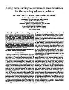
(15) and is the number of data points. This paper applies these two criteria jointly: meeting either of these two criteria indicates that the change of distance between and in going from dimension to dimension points is too large and the neighbor would be declared false. For the computation, this paper uses the value and the dimension going from one to ten. Using the time-delay determined in the previous section, the values of the percentage and are calculated and of GFNNs for data sets then plotted in Fig. 4. The value of GFNNs for the data drops , and remains zero after that. This means that the to zero at corresponding search trajectory of data can be reconstructed to represent faithfully its in an embedding dimension geometric structure. and more closely. Let us look at the time series , we can see From the curve of global false neighbors for that, as the dimension increases, the percentage of false neighbors drops and then rises, which indicates that this data comes from a dynamical process with very high dimension. However, and shows that the embedding dimension the curves for and are for the corresponding trajectories of and , respectively. This fact indicates that the dynamics of the heuristic search process changes over time. More specifically, the dimensionality of the local heuristic search process decreases over time, from high-dimensional to low-dimensional dynamics. E. Reconstruction Results The reconstruction of a trajectory can be interpreted as a process of coordinate change. Often the trajectory of a dynamical process is originally defined in some high-dimensional space. The reconstruction amounts to a projection of the original to a smaller dimensional Euclidean space. The for the embedding space guarantees chosen dimension that each point in the projected trajectory corresponds to one and only one point in the original trajectory. In other words, the reconstruction is a truthful representation of the original trajectory. There is no image where parts of the trajectory are collapsed onto each other. Thus, we should be able to extract full information about the geometric structure from a single-variable time series, using the time-delay reconstruction. One of the problems of state space representation is the deficiency in our brains that prevents us from visualizing dimensions for greater than three. Because of this limitation, two-dimensional (2-D) or three-dimensional (3-D) space is still a common medium for communication about -dimensional problems worked out in our heads. This paper reconstructs the heuristic search trajectory on a 3-D plot, using the time-delay suggested by the average mutual information; even the calare larger than culated values of the embedding dimension three. The 3-D reconstructed trajectory is not identical to the
Fig. 4. Curves of global false nearest neighbors (GFNNs) for D; D1; D2; and D3. The embedding dimensions for D; D 2; and D 3 are m = 4; 6; and 5, respectively. The embedding dimension for D 1 is very high.
original but more or less a distorted copy. This kind of dimensional reduction is forced on us by our presentation instrument and also is employed as a way of reducing complexity since our brains are so limited. Certainly, some information about the trajectory is lost in this dimension-reduced representation. However, just because some information is lost does not mean that the visual representation is useless. The reconstructed trajectory still provides information about the dynamical structure of the process. Fig. 5 portrays the reconstructed trajectories for the data sets and . These portraits provide a geometric representation of complex dynamics of the local search system. The search trajectory has a loose structure at beginning [part (b)], which means the search process has more opportunities to find better solutions and thus has fast convergent speed. The middle part of the trajectory [part (c)] shows that the structure becomes tight, which means that the process has to take longer time searching neighbors to find a better solution. The lower part ([part (d)] reveals even an tighter structure, like a thread ball, which means that the search activity is restricted in an even smaller domain. Data visualization is a process of transformation of data into a picture, which engages the interaction of human visual system with the spatial organization of the data. The result is a simple, effective, and eye-pleasing graphic medium for communicating complex information. The time series generated by the Or-opt system can be used to visualize the solution space explored by the search process. This time series has three characteristics. First, it is discrete. The implication of this characteristic is that the character of the data between discrete points unknown. However, we often need information at positions other than the supplied points for graphic rendering. One of important visualization activities is to determine data value at an arbitrary position. Interpolation is a widely used technique. This method interpolates data from points to some intermediate point using interpolation functions that presume a relationship between neighboring data values. Often this is a linear function, but it can be a quadratic, cubic, spline, or other function.
LI AND ALIDAEE: DYNAMICS OF LOCAL SEARCH HEURISTICS FOR TRAVELING SALESMAN PROBLEM
179
Fig. 5. Search trajectory of the Or-opt heuristic system. (a) shows the search trajectory for data , (b) shows the trajectory for data 1, which is a subset of , and (c) and (d) show the trajectories for data 2 and 3, respectively.
D
D
D
D
D
Another characteristic of the data is its irregularity. The points in an irregular data set are irregularly located in space and have no inherent structure. The geometry is unstructured. An irregular data set must be explicitly represented. This requires greater memory and computational resources. However, the advantage of irregular data is that irregular data gives us more freedom in representing it. Data can be represented in such a way that no regular patterns can be found in topology or geometry. However, for the purpose of visualization, an irregular data is typically transformed into a structured form. Finally, the third important characteristic of the data is its dimension. For example, as calculated in the previous section, is very high. However, the embedding dimension for data people usually use a surface in three dimensions to represent a state space. Data visualization deals with the issues of data transformation and representation. Transformation is the process of converting data from its original form into computer image. Representation is both the internal data structure used to depict the data and the graphics used to display the data. In this paper, the structural representation of the data is a matrix of solution values, while the graphical representation of the data is a surface in 3-D space. Thus, the solution space is created in a 3-D Cartesian space from a time series that is actually embedded in a higher dimension. along the Each point is expressed as a triplet of values - -, and -axes. The primary task of visualization in this paper is to transform the data from scalars into vectors and to specify data geometry (i.e., point coordinate). The time series data are matrix. Suppose the size of the time sampled on a regular matrix is created such that . One series is , the matrix defines the values along only one axis. Therefore, three matrices, and , are created to specify the solution surface. These three matrices provide a structured frame for defining the position of the vectors. Specifically, matrices and together return a list of triples specifying vector points in 3-D space, which in turn defines rectangular grids on the surface. Each point in the rectangular grid can be thought of as connected to its three nearest neighbors. This underlying rectangular grid induces four-sided patches on the surface. Then,
Fig. 6. Solution surface space explored by the Or-opt heuristic search system during its first 1000 searches.
the patches are filled with color. This paper uses the ready-made 3-D surface visualization tools in MATLAB. Fig. 6 shows the , which can be considsolution surface built from the data ered as the local solution space searched by the Or-opt search system during its first 1000 iterations. IV. THE DYNAMICS OF THE SEARCH SYSTEM A. The Correlation Dimension Generally speaking, the analysis of dynamical behavior is extremely difficult. The goal of trajectory reconstruction is to capture the geometric pattern of points on a trajectory of a dynamical process [15]. There is also a need to define quantitatively dynamical properties of heuristic search system. In characterizing a dynamical process quantitatively, the emphasis is on the time-dependent dynamical behavior of the system and the geometric nature of the trajectories in the state space. One approach to characterize the temporal dynamics of a system is to calculate the dimension of the process trajectory. The dimensionality of the trajectory is closely related to dynamics of the system [31], since the dimensionality of a process gives us an estimate of the number of active degrees of freedom in the system. This paper uses the correlation dimension technique to investigate the dynamical structure of the Or-opt search system, and shows how to extract a multidimensional description of dynamics of a solution space from a single-variable time series. The determination of the fractal dimension of a trajectory has become a standard diagnostic tool in the analysis of a dynamical system. The dynamical complexity of a system can be described by the calculated dimension of its trajectory.The most recent work in characterizing dynamical process has focused on the evaluation of fractal dimension by calculating the correlation dimension. The correlation dimension is originally due to Grassberger and Procaccia [32]. It becomes a popular technique because of its simplicity, computational speed, and minimal storage requirement.
180
IEEE TRANSACTIONS ON SYSTEMS, MAN, AND CYBERNETICS—PART A: SYSTEMS AND HUMANS, VOL. 32, NO. 2, MARCH 2002
Correlations between points on a trajectory are defined in terms of spatial correlation that can be formally measured by the Euclidean distance. The correlation dimension considers the statistics of distances between pairs of points [33]. The procedure of estimating the correlation dimension from a single-variable time series is as follows. 1) The time series are embedded in successively increasing dimensions as prescribed by Takens [34]. The series of scalars is converted into a series of vectors in each embedding dimension . 2) For each embedding dimension, the correlation integral is computed and then the correlation exponent is estimated. 3) The procedure is repeated until the estimates of converge. 4) Whatever value at which remains stable over a number of embedding dimensions is taken as the estimate of the for the underlying trajectory. correlation dimension measures the spatial correlation The correlation integral , among the points on a trajectory. Specifically, for each is defined as the average number the correlation function that are separated by a distance of pairs of data vector less than the number of pairs such that
(16)
where denotes the number of points on the trajectory. In principle, should go to infinity, but in practice is limited by the denotes the distance availability of the time series points. The induced by the selected norm. According to Theorem 2.4 of Brock [35], the correlation dimension is independent of the choice of norm. Thus, the Euclidean distance is used in this paper. measures the probability that any particIntuitively, ular pair in the time series is close. Grassberger and Procaccia [32] have established that the true spatial correlation grows ac, cording to the power law, that is, for small values of grows exponentially at the rate of (17) where is the correlation exponent. If tends to be a constant as increases, then yields an estimate of embedding dimension the correlation dimension of the trajectory. In this case, the data are consistent with deterministic behavior. If increases without increases, this suggests bound as the embedding dimension that the data is stochastic as the dimension of the dynamical process approaches infinity. is defined to be the Therefore, the correlation dimension number that satisfies (18) Then, the correlation dimension
is obtained by (19)
if the limit exists. is defined as a function of such that inIn (16), creases from zero to one as increases from zero to . In other words, if all the data points are within the distance of each
other, then . If is smaller than the smallest distance . Since any real data set between trajectory points, then consists of a finite number of points, it is not possible to take the and . Hence, in practice, the correlation limits dimension is found using some range of values and plotting as a function of . In this way, a plot of versus is produced. We can observe that only in some intermediate region does obey the power law expressed in (18) [36]. This region is called the scaling region, and the curve in this region is approximately a straight line. The slope for the curve from (19) without the determines the correlation dimension . limit Since in practice the presence of noise in a data is likely to reversus , sult in a choppy appearance in the curve of we often need to run a linear regression on the curve. The slope estimate from this regression is the correlation dimension estimate for this value of . Therefore, there are some uncertain, which can cause the computed ties involved in calculating dimension to differ slightly from the “true” value. This procedure is repeated for a sequence of increasing values of . If the time series are purely random, then in infinite data . In practice, sample, the correlation dimension will equal with a finite data set, the correlation dimension estimate may at less than a one-for-one rate [37]. If the time serise with should iniries are deterministic, the correlation dimension tially increase with increasing values of . However, at some should level off and remain constant for all furpoint, . One should observe a “plateau” on the plot ther values of in the function of embedding of the correlation dimension dimension . This “saturation” value of the slope is the correlation dimension estimate for the underling system that generates the data. In practice, the slope estimate may never completely stop rising. Thus, the process of determining whether saturation has occurred can, in general, be rather judgmental. Ding et al. [38] reported that, for a large enough data set, the saturation begins first exceeds the when the number of embedding dimension . However, a lack of sufficient data will delay the correlation saturation onset. Taken’s theorem [34] provides a practical clue. The embedding theorem shows that if the true system that generated the time series is in dimension, the embedding space dimension to capture completely needs to have the dynamics of the underlying system. Since is unknown, an values must be tried. Usually, has increasing sequence of before the value deduced for to be increased to nearly become independent of . B. Empirical Results Fig. 7 illustrates a plot of the natural logarithm of the correfor different values of for lation integral as a function of the data . The curves correspond to computation of the cor. relation function in embedding dimension The values of are experimentally determined in the following represent the size of the trajectory under conmanner. Let sideration, which can be obtained from (15), then is calculated as (20)
LI AND ALIDAEE: DYNAMICS OF LOCAL SEARCH HEURISTICS FOR TRAVELING SALESMAN PROBLEM
181
Fig. 8. Comparison of correlation dimensions between the heuristic time series D and the random data.
Fig. 7. Correlation integers in different embedding dimension 1; 2; . . . ; 10 for the data D .
d
=
TABLE I THE SLOPE OF EACH CURVE IN FIG. 7
where the values of and are chosen experimenvalues that would encomtally to provide a range of pass a nearly linear region of the curve. This study by using a trial-and-error program. selects The proportion that lie within the range is counted for , which make 20 points on the curve. In this way, a series of correlation dimensions is calculated over ten embedding dimensions and plotted. Then, the slope for each curve is found by the least squares regression and shown in Table I. As a practical matter, we search to see whether the values as embedof correlation dimension stabilize at some value increases. If so, then the value is the ding dimension is a small value, then the correlation dimension estimate. If process is substantially deterministic even it is complicated. If, increases, the correlation dimension continues however, as to increase at the same rate, then the process is taken to be stochastic. In principle, an independently and identically distributed stochastic system is infinite dimensional. Each time one increases one available degree of freedom, the random system utilizes that extra freedom. Therefore, it is desirable to calculate the correlation dimension for a “random” system to provide a basis for comparison. Fig. 8 compares the correlation dimensions of the time series with the correlation dimensions of a random data, which consists of 10 000 data points that are
uniformly distributed over the interval [1, 1000]. As shown in for the data stabilizes Fig. 8, the correlation dimension when the embedding dimension is greater than about twice the correlation dimension of the data, indicating that the correlation . The saturated correladimension becomes independent of for the data is determined tion dimension value . For the random-number data, no at the corresponding saturated correlation dimension can be found. contains The correlation dimension estimate for the data information about the dynamics of the heuristic search process during its first 10 000 searches. This value describes an averaged property of the search process. In other words, this correlation dimension is an average measure over the entire search trajectory (10 000 points). However, Fig. 5 reveals that, in the heuristic search process, the hill-climbing phase has a different geometric structure from the plateau phase’s, indicating different levels of dynamics of search motions. The local contributions from different parts of the search trajectory to the average dynamics are, in general, different. Just an average value does not acknowledge all of the complexity of the search process. We ask what happens to the dynamics of the search trajectory if we examine it at different parts. Thus, this study divides the 10000-points trajectory into ten parts, each consisting of 1000 points. It is expected that different parts of the search trajectory to be characterized by different values of the correlation dimension. The heuristic search trajectory should be an object with a multiplicity of fractal dimension. Fig. 9 shows a schematic graph of the correlation dimension as a function of the embedding dimension for five partitions of the heuristic time series. For comparison, the correlation dimension for a 1000-points random data is also plotted. We can see that, although the curve of correlation dimension for the first 1000 data points are below the curve for the random , there is no sign of saturation, indicating data, up to that the time series for this partition are indeed of high, if not infinite, dimension. It indicates the presence of a stochastic search process during the first 1000 searches. However, the correlation dimension of search process decreases as the search continues, indicating that the complexity of search dynamics appears to decrease as the heuristic search is approaching to a local optimal point. In summary, in the course of searching for an optimal solution on the solution space, the dynamics of the heuristic search process changes from a stochastic process to a process with low-dimensional structure.
182
IEEE TRANSACTIONS ON SYSTEMS, MAN, AND CYBERNETICS—PART A: SYSTEMS AND HUMANS, VOL. 32, NO. 2, MARCH 2002
TABLE II ITERATIONS AND BETTER SOLUTIONS
Fig. 9. data.
Correlation dimensions for the partitions of heuristic data and random
V. CONCLUSION AND DISCUSSION This paper reconstructs a search trajectory for the Or-opt heuristic search system on the TSP. The trajectory illustrates the graphical representation of the dynamical process of the search system in its solution space. The critical aspect of the time-delay coordinates is that the dynamical behavior of a local search process can be reconstructed from a time series data. The dynamics of the search process can be seen by the picture of the data. In fact, a collection of many such search trajectories originating from different initial points can portray the entire solution space for the search system. This paper also uses the correlation dimension technique to quantitatively characterize the complexity of the dynamics for the search system. The results reveal that the heuristic search process exhibits the transition from high-dimensional stochastic to low-dimensional chaotic behavior. The initial phase of search process shows more complexity in dynamics than the later phases of the search. The heuristic search process starts with a high-dimensional searchable space. However, the dimension of the searchable space is rapidly reduced. As the search is approaching to a local optimal point, the searchable space becomes smaller and smaller. This decomlexification of search dynamics appears to be a generic response to perturbation associated with the solution configuration. A local heuristic search process searches for an optimal configuration by repeatedly moving from the current configuration to a neighboring configuration. In the early stage of search, the frequency of this configuration perturbation is very high. However, the possibility of finding a better configuration is less and less as the search goes on. Thus, the loss of complexity, as assessed by the measurement of correlation dimension, can be related with this decreasing possibility. The search process looks very much like passing through many levels of laminar. The search begins with a large laminar with many corridors. It is vary easy for the process to find a corridor to pass through to next laminar, which
is characterized by smaller size and less corridors. Every time the search process gets into a new laminar, it will take a longer time to find a corridor to pass through to the next laminar. The closer to a local optimal point, the longer the average laminar time will take. One issue related with the loss of complexity is the size of solution space that can be effectively searched. Many degrees of freedom on the first laminar are reduced to a few on the later laminars. Average degrees of freedom is increased by over the residual degrees of freedom the restriction of neighborhoods. The size of solution space that can be reached may decrease exponentially. This decreasing size of the solution space perhaps can be modeled to describe the search effectiveness for a heuristic search process. Usually, the more iterations we perform the better final solution we can get. But how many iterations are enough? It is perhaps somewhat surprising that there does not yet exit a useful convergence theory for this question. Let us assume that after, say 175 321 iterations, we found another better solution. However, is it the last one we will find it if we continue to iterate? There is no way to tell. However, still we must make a decision. For example, we can propose to perform another 10 000 iterations, and if we do not find any more new better solution, we may be content and stop the iteration. However, probably only the next iteration beyond the 10 000 may prove that we are wrong in this assumption. Table II illustrates the results of an experiment. This experiment applies the Or-opt algorithm on three uniformly distributed TSP instances with 1000, 2000, and 4000 cities, respectively. One million iterations are performed on each instance. The number of better solutions found (i.e., the times of solution configuration perturbations) iterations is recorded. during We can see that, for example, for the 1000-city instance, 242 better solutions are found in the first 10 000 iterations and another eight better solutions in the next 90 000 iterations, but no more better solutions found in the next 900 000 iterations. In the 2000-city case, 471 better solutions are found in the first 100 000 iterations and another five better solutions in the next 900 000. How many more iterations should we perform to produce one more better solution? Even if the case of simple local search iterations are very cheap, for a very large problem instance, the number of iterations needed for a satisfied solution may be typically in the order of tens of millions. For many other more sophisticated search heuristics, one million iterations may be well above any reasonable computational time frame. Thus, the problem outlined above really exists in practice, and a solution should be sought. We have known that this problem may be associated with the loss of complexity in the search process. Correlation dimension technique may help us to capture the relevant frequencies or time scales for a particular heuristic search process. Then, an expected number of better
LI AND ALIDAEE: DYNAMICS OF LOCAL SEARCH HEURISTICS FOR TRAVELING SALESMAN PROBLEM
solutions found during iterations, given the size of the , may be predicted by a map . Such problem a search effectiveness model may answer the question whether we are finding an adequate solution within a time acceptable to the situation, for this size of problem instance, when using this particular search heuristic. Thus, if a heuristic user can expect how many better solutions will be produced during the next, say 100 000 iterations, one has great flexibility in deciding whether or not to trade solution quality for time. Although this paper investigates the dynamical behavior of the Or-opt heuristic in the TSP, the results appear to be behavioral archetypes for the class of local search heuristics in combinatorial optimization problems generally. There is no strict mathematical definition to describe the behavior of the heuristic search process concisely. The process exhibits complicated patterns in both space and time. Suppose that, for a heuristic search system, the initial conditions are confined to some volume in solution space bounded by a “surface” of all initial points. As the process evolves, the volume will move through solution space, which looks like the motion of compressible object. The shape of the volume will be distorted, and the size will be decreased. The final volume occupied by the set of local optimal points is very small. This small volume is called a solution attractor. All search trajectories will be attracted to this volume. In fact, there are two competing effects present in the heuristic search process. In one, due to the sensitive dependence on initial conditions, two different search trajectories will diverge. On the other hand, the trajectories must converge to a finite region of the solution space. It is clear that the initial segment of search trajectory is a kind of “coherent randomness.” This randomness is subdued by some modulation. After certain search iterations, this randomness is quickly replaced by a low-dimensional mode of chaos. Then, the search process continues to be suppressed slowly by the modulation over a long period of time. Finally, when the system reaches some local optimal configuration, the chaos is replaced by a quasi-periodic mode of motion. In the classical picture of statistical mechanics, it is believed that a large number of degrees of freedom are necessary for ergodicity [39]. When a heuristic search process is in the stochastic motion stage, it has the ability to explore wide regions of the solution space, and thus to utilize information about a large collection of potential solutions of the process. When the process gets into the chaotic stage with a few degrees of freedom, it explores a very limited domain of solution space. The search activity now is rather restrictive. The distribution of solution space being searched is far from “equipartition” and is replete with high-probable regions. In summary, a local search process can start from different initial points in solution space and finally wind up at a small attracting region in the solution space. No wonder Boese et al. [40], [41] found a “big valley” structure governing the set of local minimums. Their research shows the evidence that “very good solutions are located near other good solutions.” In fact, it is the attracting region that creates a globally convex structure for the set of local minimums in the optimization solution space. This kind of asymptotic behavior of the heuristic search process can have distinct implications for a wide range of theoretical and practical problems in heuristic theory, design, and analysis.
183
REFERENCES [1] C. H. Papadimitriou and K. Steiglitz, Combinatorial Optimization: Algorithms and Complexity. Englewood Cliffs, NJ: Prentice-Hall, 1982. [2] L. K. Grover, “Local search and the local structure of NP-complete problems,” Oper. Res. Lett., vol. 12, pp. 235–243, 1992. [3] C. H. Papadimitriou and K. Steiglitz, “On the complexity of local search for the traveling salesman problem,” SIAM J. Comput., vol. 6, pp. 76–83, 1977. [4] C. R. Reeves, Modern Heuristic Techniques for Combinatorial Problems. New York: Wiley, 1993. [5] “The design, analysis, and implementation of heuristics,” Manage. Sci., vol. 34, no. 3, pp. 363–429, 1988. [6] S. H. Zanakis, J. R. Evans, and A. A. Vazacopoulos, “Heuristic methods and applications: A categorized survey,” Eur. J. Oper. Res., vol. 43, no. 1, pp. 88–110, 1989. [7] S. E. Elmaphraby, “A graph theoretic interpretation of the sufficient conditions for the contiguous binary switching (CBS) rule,” Nav. Res. Logist., vol. 18, no. 3, pp. 339–344, 1971. [8] J. R. Evans, “Structural analysis of local search heuristics in combinatorial optimization,” Comput. Oper. Res., vol. 14, no. 3, pp. 465–477, 1987. [9] L. K. Grover, “Local search and the local structure of NP-complete problems,” Oper. Res. Lett., vol. 12, no. 4, pp. 235–243, 1992. [10] P. Gent and T. Walsh, “An empirical analysis of search in GAST,” Univ. of Edinburgh, Artif. Intell. Dept., Edinburgh, U.K., 1993. [11] I. Or, “Traveling salesman-type combinatorial problems and their relation to the logistics of regional blood banking,” Ph.D. dissertation, Northwestern Univ., Evanston, IL, 1976. [12] H. Tong and K. S. Lim, “Threshold, autoregression, limit cycles, and cyclical data,” J. Roy. Stat. Soc., vol. 42, no. 3, pp. 245–292, 1980. [13] K. T. Alligood, T. D. Sauer, and J. A. Yorke, Chaos: An Introduction to Dynamical System. New York: Springer-Verlag, 1997. [14] E. Ott, T. Sauer, and J. A. Yorke, Eds., Coping with Chaos: Analysis of Chaotic Data and the Exploitation of Chaotic Systems. New York: Wiley, 1994. [15] N. Packard, J. P. Crutchfield, J. D. Farmer, and R. S. Shaw, “Geometry from a time series,” Phys. Rev. Lett., vol. 45, no. 9, pp. 712–716, 1980. [16] F. Takens, “Detecting strange attractors in turbulence,” in Dynamical Systems and Turbulence, Warwich 1980, Lecture Notes in Mathematics, 898, D. Rand and L. S. Young, Eds. New York: Springer-Verlag, 1981, pp. 366–382. [17] H. D. I. Abarbanel, Analysis of Observed Chaotic Data. New York: Springer-Verlag, 1996. [18] H. D. I. Abarbanel, R. Brow, J. J. Sidorowich, and L. S. Tsimring, “The analysis of observed chaotic data in physical systems,” Rev. Mod. Phys., vol. 65, no. 2, pp. 1331–1392, 1993. [19] D. S. Broomhead and G. P. King, “Extracting qualitative dynamics from experimental data,” Phys. D, vol. 20, no. 1, pp. 217–221, 1987. [20] M. Casdagli, T. Sauer, and J. A. Yorke, “Embedology,” J. Stat. Phys., vol. 65, no. 3/4, pp. 579–616, 1991. [21] H. D. I. Abarbanel and J. B. Kadtke, Information Theoretic Methods for Choosing the Minimum Embedding Dimension for Strange Attractors. San Diego: Inst. Nonlinear Sci., Univ California, 1989. [22] A. M. Frazer, “Information and entropy in strange attractors,” IEEE Trans. Inform. Theory, vol. 35, no. 2, pp. 245–262, 1989. [23] A. M. Frazer and H. L. Swinney, “Independent coordinates for strange attractors from mutual information,” Phys. Rev. A, Gen. Phys., vol. 33, no. 2, pp. 1134–1140, 1986. [24] A. Cenys and K. Pyragas, “Estimation of the number of degrees of freedom from chaotic time series,” Phys. Lett. A, vol. 129, no. 4, pp. 227–230, 1988. [25] W. Liebert and H. G. Schuster, “Proper choice of the time-delay for the analysis of chaotic time series,” Phys. Lett. A, vol. 142, no. 2/3, pp. 107–111, 1989. [26] T. Buzug, T. Reimers, and G. Pfister, “Optimal reconstruction of strange attractors from purely geometrical arguments,” Europhys. Lett., vol. 13, no. 7, pp. 605–610, 1990. [27] R. S. Shaw, The Dripping Faucet as a Model Chaotic System. Santa Cruz, CA: Aerial, 1985. [28] R. G. Gallager, Information Theory and Reliable Communication. New York: Wiley, 1968. [29] C. E. Shannon and W. Weaver, The Mathematical Theory of Communication. Urbana, IL: Univ. Illinois Press, 1949.
184
IEEE TRANSACTIONS ON SYSTEMS, MAN, AND CYBERNETICS—PART A: SYSTEMS AND HUMANS, VOL. 32, NO. 2, MARCH 2002
[30] M. B. Kennel, R. Brown, and H. D. I. Abarbanel, “Determining embedding dimension for phase-space reconstruction using a geometrical construction,” Phys. Rev. A, Gen. Phys., vol. 45, no. 6, pp. 3403–3411, 1992. [31] R. C. Hilborn, Chaos and Nonlinear Dynamics: An Introduction for Science and Engineers. London, U.K.: Oxford Univ. Press, 1994. [32] P. Grassberger and I. Procaccia, “Characterization of strange attractors,” Phys. Rev. Lett., vol. 50, no. 5, pp. 346–349, 1983. [33] T. S. Parker and L. O. Chua, Practical Numerical Algorithms for Chaotic Systems. New York: Springer-Verlag, 1990. [34] F. Taken, “On the numerical determination of the dimension of an attractor,” in Dynamical Systems and Bifurcations, N. Breaksma, H. Broer, and F. Takens, Eds. New York: Springer-Verlag, 1985, pp. 99–106. [35] W. Brock, “Distinguishing random and deterministic systems: Abridged version,” J. Econ. Theory, vol. 40, no. 1, pp. 168–195, 1986. [36] J. Holzfuss and G. Mayer-Kress, “An approach to error-estimation in the application of dimension algorithm,” in Dimensions and Entropies in Chaotic Systems: Quantification of Complex Behavior, G. Mayer-Kress, Ed. New York: Springer-Verlag, 1986, pp. 114–122. [37] J. B. Ramsey and H. J. Yuan, “The statistical properties of dimension calculations using small data sets,” C. V. Starr Center, New York Univ., New York, Res. Rep. 87-20, 1987. [38] M. Ding, C. Grebogi, E. Ott, T. Sauer, and J. A. Yorke, “Plateau onset for correlation dimension: When does it occur?,” Phys. Rev. Lett., vol. 70, no. 25, pp. 3972–3975, 1993. [39] Y. Kuramoto, Ed., Chaos and Statistical Methods. New York: Springer-Verlag, 1984. [40] K. D. Boese, A. B. Kahng, and S. Muddu, “On the big valley and adaptive multi-start for discrete global optimizations,” Comput. Sci. Dept., Univ. California, Los Angeles, Tech. Rep. TR-930 015, 1993. , “A new adaptive multistart technique for combinatorial global op[41] timizations,” Oper. Res. Lett., vol. 16, no. 2, pp. 101–113, 1994.
Weiqi Li received the B.S. degree in mechanical engineering from Nanjing University of Aeronautics and Astronautics, Nanjing, China, in 1982, the B.A. degree in international trade from University of International Business and Economics, Beijing, China, in 1986, and the M.B.A. and M.S. degrees in computer science and the Ph.D. degree in management information system from the University of Mississippi, University, in 1994, 1996, and 1998, respectively. He served as Visiting Assistant Professor in the School of Business at University of Mississippi in 1999 and as Assistant Professor in the School of Business at Michigan Technological University, Houghton, from 1999 to 2001. In 2001 he joined the faculty of the School of Management of the University of Michigan, where he is currently an Assistant Professor of management information systems. His research interests include machine learning, heuristics for the combinatorial optimization problems, and e-learning.
Bahram Alidaee received the B.S. degree from the University of Tehran, Iran, the M.B.A. degree from the University of North Texas, Denton, and the Ph.D. degree in mathematical sciences from University of Texas at Arlington, in 1992. He is currently an Associate Professor of operations management at the School of Business Administration and the Hearing Center for Enterprise Science at the University of Mississippi, University. His current research interests include: design and implementation of metaheuristics for the combinatorial optimization problems, and surrogate/Lagrangean relaxation applications to verylarge-scale problems in optimization problems. He has published in various journals including Management Science, Journal of Production and Operations Management, Journal of Operational Research Society, European Journal of Operational Research, Journal of Optimization Theory and Applications, Computers and Operations Research, etc.