Nov 9, 2009 - was discussed previously, in Sections IIIB and IVB. In the former it was shown that if a local minimum of den- sity inside the BEC is small ...
Dynamics of Macroscopic Tunneling in Elongated BEC G. Dekel1 , V. Farberovich1, V. Fleurov1 , and A. Soffer2
arXiv:0911.1537v1 [cond-mat.quant-gas] 9 Nov 2009
1 Raymond and Beverly Sackler Faculty of Exact Sciences, School of Physics and Astronomy, Tel-Aviv University, Tel-Aviv 69978 Israel and 2 Department of Mathematics, Rutgers University, New Brunswick, NJ 08903,USA
We investigate macroscopic tunneling from an elongated quasi 1-d trap, forming a ’cigar shaped’ BEC. Using recently developed formalism1 we get the leading analytical approximation for the right hand side of the potential wall, i.e. outside the trap, and a formalism based on Wigner functions, for the left side of the potential wall, i.e. inside the BEC. We then present accomplished results of numerical calculations, which show a ’blip’ in the particle density traveling with an asymptotic shock velocity, as resulted from previous works on a dot-like trap, but with significant differences from the latter. Inside the BEC a pattern of a traveling dispersive shock wave is revealed. In the attractive case, we find trains of bright solitons frozen near the boundary. PACS numbers: 82.20.Xr, 03.75.Kk, 05.90.+m
I.
INTRODUCTION
In recent years, nonlinear dynamics of BEC out of equilibrium has been given a great amount of attention, mainly in looking for various nonlinear coherent structures such as dark, bright and oblique solitons, vortices and dispersive shock waves, and studying their emergence and evolution. Dark and bright solitons were first observed experimentally in Refs. 2,3,4,5. Vortices in 2d BECs were discussed in Refs. 6,7,8,9. Recently, much attention has been drawn to dispersive shock waves, which contrary to their dissipative counterparts in compressible fluid, and due to their quantum nature are controlled by the dispersion effects rather than by dissipation, and are now believed to emerge in and dictate the dynamics of BEC flow. They are characterized by an expanding oscillatory front, and, as other phenomena in BEC, are predicted and quested by the the Gross - Pitaevskii equation (GPE) i~ �
∂Ψ(r, t) = ∂t
� ~2 2 2 − ∇ + Uext (r) + N Uint | Ψ(r, t) | Ψ(r, t) 2m
(1)
Recently dispersive shock waves in different BEC setups and with various initial conditions have been investigated and predicted theoretically, as well as observed in experiments. First evidence of possible shock waves development in BEC setups were reported in10 , where a sharp density depression was induced by slow light technique. Theoretical studies showed formation of a shock front in traveling 1-d BEC wave packets, split from an initial density perturbation in Refs. 11 and 12. Shock waves in BEC induced by using Feshbach resonance were studied in Ref. 13 and Witman averaging method was used to analyze 1-d BEC shock waves in the small dispersion limit in Ref. 14. Ref. 15 presented imaging of rotating BEC ”blast waves” along with numerical analysis. A broad comparison between dispersive and dissipative shock waves in all dimensions was carried out in Ref.
16, which included examination of experimental reports and theoretical results. Study of supersonic flow past a macroscopic obstacle in 2-D BEC gave rise to predictions of a sonic Cherenkov cone that would eventually transform into spatial 2-d supersonic dispersive shock waves.17 Predictions of new 2-d creatures, called oblique solitons followed and are now an object of extensive studies in the field.18,19 . In Refs. 20,21, evidences of shock phenomena in macroscopic flow were found in nonlinear optics experiments. In our previous works1,22 we studied tunneling from a trapped BEC Gaussian packet. For this purpose we analytically solved GPE in its hydrodynamic presentation. We showed that tunneling resulted in formation of an isolated ’blip’ in the particle density outside the trap, originating from a shock-type solution of the Burgers equation and moving with the asymptotic velocity of this shock. Experimental studies of the relevant phenomena in nonlinear optics were reported in Refs. 23,24 This effect is independent of the effect of non-linearity, i.e. inter-atomic interaction in BEC or Kerr nonlinearity optics, and includes the case in which the latter is zero.1 . This effect can be made repeatable in time by periodically bringing the potential walls closer (or changing the trap frequency) thus releasing additional blips with feasible control of their parameters, which may lead to an eventual realization of atom soliton laser.22 Since a strongly trapped BEC packet,(i.e. the margins of the trap are of the same order of magnitude as its bulk in all directions) reacts to tunneling in pulsations inside the trap, with frequency which is twice the in-trap eigen frequency, this periodicity is used to determine the timing of the mechanism described above. Sudden turn-on of a matter-wave source in order to create repeated pulses was discussed in Ref. 25. This paper will investigate tunneling from a quasi 1d cigar shaped trap with a twofold motivation: Firstly, we intend to look for the emergence of a single blip and its properties in order to eventually create a pulsed atom laser on the basis of this system, providing a much greater source of matter than in the previous case of tunneling
2 III. A.
wave function Potential barrier
ANALYTICAL RESULTS
Right hand side of the barrier
Wave function\Potential
In our previous work1 we introduced a formalism that solves GPE with a given external potential, in the hydrodynamic representation. The GPE is equivalently written in the form of the Euler type 1 1 vt + ∇v 2 = − 2 m
−100
0 x
100
FIG. 1: A schematic arrangement of the investigated problem. At t = 0, the potential wall narrows down to a finite width barrier, enabling the cigar shaped BEC tail to tunnel
from a trapped narrow packet (tightly trapped in all directions). Our second aim is to investigate the opposite effect, i.e. the dynamics inside the BEC cigar shaped trap, which appears to be much richer. We will show that an ”anti-blip” (a local depletion) is formed, which propagate inside the trap with the same velocity as the blip outside but in the opposite direction. However the structure and development of this anti-blip is very complicated and in particular it may develop into a dispersive shock wave. II.
MODEL AND FORMALISM
� 2 2√ � ~ ∇ ρ − √ + Uext + N Uint 2m ρ
(2)
ρt + ∇(ρv) = 0.
(3)
and continuity
equations. Then the Euler equation (2) is solved under an adiabatic approximation according to which the density field ρ = |Ψ|2 evolves with the time of tunneling τtun whereas the velocity field mv = ∇ϕ (ϕ being the gradient of the phase of wave function Ψ) with the traversal time τtr satisfying the condition τtun ≫ τtr . The problem of a quantum fluid dynamics can be mapped onto that of a classical dissipationless fluid motion. We found out that solving the first iteration actually sufficed to investigate short and long time dynamics of the problem. To investigate the dynamics outside the barrier in the present work, the analysis can be therefore made, as in the previous works1 by solving the classical integral Z x dξ q t= (4) 2 x0 (ǫ − U (ξ)) m where
We consider the following physical system. An elongated 1d wave-function is sealed on its right hand side by a high enough wall, i.e. U0 > N Uint | ψ(r, t) |2 . (The quantum pressure term is always negative around the barrier region) The wall is lowered, at t = 0, so that a tail of the wave function is allowed to tunnel and dynamically evolve according to the GPE through the new barrier of a finite width, the height of its peak is that of the former wall. This is shown in Fig. 1. We solve the 1-d GPE (1) numerically and analytically for the right and left sides of the barrier respectively, after t = 0.
U (ξ) = Ut=0− (ξ) − Ut=0+ (ξ) =
1 U0 (1 − tanh(αξ) (5) 2
is the difference between the potential shapes before and after switching from a wall to a barrier of finite width. t is the time required for a fluid droplet (tracer) to reach the point x and have velocity v, if it has started from the point x0 with the energy ǫ. Assuming that initially the fluid was motionless v0 = 0 at t = 0, i.e. ǫ = mv 2 /2, we get
q 1 q 1 ǫ− 2 U0 + 12 U0 tanh(αx) ǫ− 2 U0 + 12 U0 tanh(αx) arctanh( ) arctanh( ) ǫ−U0 ǫ √ √ + αt(x, ǫ) = ǫ ǫ − U0
¿From here, one can find ǫ(x, t) numerically and therefore the velocity field v(x, t). The results are shown in Fig.
(6)
2 and indicate, as expected, a tendency to shock wave formation (compare Refs. 1,22) to result in a blip in the
3 density distribution. The time scale of its creation is 4 time units (traversal times τtr ) which matches that of the blip formation time to be obtained numerically. B.
Left hand side of the barrier
To deal with the dynamics to the left side of the barrier (inside the BEC) analytically, one can derive a hydrodynamic ”hole representation” by means of Wigner function technique. For this, let us assume that we have a homogeneous density distribution ρ0 and consider fluctuations changing this density. In this case we have to define a ”hole Wigner function” as h fW (r, p, t)
which governs the dynamics of Wigner function,26 where H(r, p) =
p2 + V (r) 2m
is the classical Hamiltonian of the system. The definition of the ⋆ product and detailed discussion can be found in Ref. 27. Multiplying equation (11) by pα and integrating over p we get − m0
−
=
∂ [ρh (r, t)vhα (r, t)] = ∂t
∂V (x) 1 ∂ β ρ(r, t)δ αβ + [ρh (r, t)pα h ph ] ∂xβ m0 ∂xβ
(12)
Then using the continuity equation (10) we write Z
d3 y [−ψ(x − y/2, t)ψ ∗ (x + y/2, t) + ρ0 ] eipy/~ = (2π~)3 −fW (r, p, t) + ρ0 δ(p).
� � ∂vhα (r, t) ∂ β −m0 ρh (r, t) −m0 ρh (r, t) vh (r, t) β vhα (r, t) = ∂t ∂x
(7)
We define the hole density by integrating (7) over the momentum p Z h ρh (r, t) = d3 pfW (r, p, t) = −ρ(r, t) + ρ0 (8) The hole velocity field is defined as Z α h (r, p, t) = m0 ρh (r, t)vh (r, t) = d3 p pα fW
io h ∂V (x) 1 ∂ n β α β ρh (r, t) pα ρh (r, t) + h ph − ph ph α β ∂x m0 ∂x (13) Till now no approximations have been made. But now we need an approximation that the holes can be described by i the single wave function ψh (r, t) = fh e− ~ Sh which can be justified for small values of the hole density ρh (r, t)