PROTEINS: Structure, Function, and Genetics 40:512–524 (2000)
Dynamics of Proteins Predicted by Molecular Dynamics Simulations and Analytical Approaches: Application to ␣-Amylase Inhibitor Pemra Doruker, Ali Rana Atilgan, and Ivet Bahar* Polymer Research Center, School of Engineering, Bogazici University, and TUBITAK Advanced Polymeric Materials Research Center, Bebek, Istanbul, Turkey
ABSTRACT The dynamics of ␣-amylase inhibitors has been investigated using molecular dynamics (MD) simulations and two analytical approaches, the Gaussian network model (GNM) and anisotropic network model (ANM). MD simulations use a full atomic approach with empirical force fields, while the analytical approaches are based on a coarsegrained single-site-per-residue model with a singleparameter harmonic potential between sufficiently close (r < 7 Å) residue pairs. The major difference between the GNM and the ANM is that no directional preferences can be obtained in the GNM, all residue fluctuations being theoretically isotropic, while ANM does incorporate directional preferences. The dominant modes of motions are identified by (i) the singular value decomposition (SVD) of the MD trajectory matrices, and (ii) the similarity transformation of the Kirchhoff matrices of interresidue contacts in the GNM or ANM. The meansquare fluctuations of individual residues and the cross-correlations between domain movements retain the same characteristics, in all approaches— although the dispersion of modes and detailed amplitudes of motion obtained in the ANM conform more closely with MD results. The major weakness of the analytical approaches appears, on the other hand, to be their inadequacy to account for the anharmonic motions or multimeric transitions driven by the slowest collective mode observed in MD. Such motions usually suffer, however, from MD sampling inefficiencies, and multiple independent runs should be tested before making conclusions about their validity and detailed mechanisms. Overall this study invites attention to (i) the robustness of the average properties (mean-square fluctuations, cross-correlations) controlled by the low frequency motions, which are invariably reproduced in all approaches, and (ii) the utility and efficiency of the ANM, the computational time cost of which is of the order of “minutes” (real time), as opposed to “days” for MD simulations. Proteins 2000;40:512–524. ©
2000 Wiley-Liss, Inc.
Key words: correlated fluctuations; molecular dynamics simulations; -proteins; Gaussian network model; anisotropic effects; principal component analysis ©
2000 WILEY-LISS, INC.
INTRODUCTION The biological function of proteins is generally controlled by cooperative motions or correlated fluctuations involving large portions of the structure.1–5 There exists a multitude of computational methods in the literature for identifying the dominant correlated motions in macromolecules.1,3,6 –17 The basic approach common in these studies is to decompose the dynamics into a collection of modes of motion, remove the “uninteresting” (fast) ones, and focus on a few low frequency/large amplitude modes which are expected to be relevant to function. A classical approach for determining the modes of motion is the normal mode analysis (NMA). NMA has found widespread use in exploring proteins’ dynamics starting from the original work of Go and collaborators, two decades ago. It is based on the diagonalization of the second-derivative potential energy matrix,6,18,19 assuming that harmonic potentials operate near equilibrium coordinates. The method has later been extended into a quasiharmonic oscillator approximation which utilizes, as input, the fluctuations (auto- and cross-correlations) observed in molecular dynamics (MD) simulations, thus including the effects of anharmonicity.7,20,21 The process of extracting the dominant collective modes, or the essential dynamics14,22 from fluctuations seen in MD trajectories—also called principal component analysis (PCA),23 or the molecular optimal dynamics coordinates analysis2—is now an established computational means of studying proteins’ dynamics.5 The major shortcoming of this approach is the sampling inefficiency of MD simulations. The sampling problem becomes increasingly important as the size of the investigated molecular system increases, as shown by projecting the MD trajectory onto the first few PCs.24, 25 The Gaussian network model (GNM) approach was recently proposed as a simple but extremely efficient analytical tool for modeling the dynamics of folded proteins.26 The structure is viewed as a completely elastic network, the nodes of which are the ␣-carbons, and the springs/chains are the bonded or nonbonded interactions between sufficiently close (r ⱕ 7.0 Å) residue pairs. The cutoff distance rc ⫽ 7.0 Å includes all neighbors within a *Correspondence to: I. Bahar, Polymer Research Center, School of Engineering, Bogazici University, Bebek 80815, Istanbul, Turkey. E-mail:
[email protected] Received 20 January 2000; Accepted 13 April 2000
COOPERATIVE MOTIONS IN PROTEINS
first coordination shell.27,28 Following Tirion’s original proposition,29 a single parameter (␥) harmonic potential is assigned to all pairs of residues, the absolute value of which is to be adjusted from comparison with experiments. Despite its simplicity, the GNM reproduces very closely the X-ray crystallographic Debye-Waller factors,26 the H/D exchange free energy costs,30 and the NMR relaxation order parameters,31 of individual residues in a diversity of proteins. Its major utility lies in its application to large systems. Quaternary structures that would necessitate enormous amounts of computation time if examined by MD can be analyzed within seconds (CPU time) with the GNM. The mechanisms of concerted motions in complexes such as HIV-1 reverse transcriptase with bound DNA,32 tRNA with its cognate synthetase,33 or enzymes comprising multiple subunits, such as Trp synthase having over 1,000 residues,34 were recently elucidated, consistent with experimental data. Major criticism of the GNM is its inadequacy to describe anharmonic fluctuations. This is a deficiency common to GNM and NMA. In the present paper, we investigate the dynamics of a -protein, ␣-amylase inhibitor tendamistat, using both MD simulations, and GNM analytical solution. MD trajectories will be analyzed by singular value decomposition (SVD) technique,35 a tool that proved useful for studying protein dynamics.17 We will extract here the nonlinear modes along the singular vectors— counterparts of the principal axes in PCA—and compare these to GNM modes. Finally, a new analytical method will be introduced, referred to as the anisotropic network model (ANM), which will permit inclusion of the effect of anisotropy in the network model of proteins, as this effect has proved to produce significant enhancements in the positional fluctuations, especially for larger amplitudes associated with lower frequencies.36 The type of information that will be provided by the present study is twofold. First, information on the dynamics of a protein representative of a distinct fold according to SCOP37 will be found. The so-called ␣-amylase inhibitor fold is a sandwich of two -sheets composed each of three strands. Both X-ray and NMR studies of the structure of tendamistat are available, but no theoretical study of the dynamics of this family has been performed to date. An assessment of the regions involved in concerted motions and residues modulating the cooperative fluctuations will be made here using MD simulations, and the exact solutions from the GNM and ANM theories. The analysis will also serve to suggest the sites prone to disruptive mutations. The second issue to be addressed relates to an assessment of the utilities and/or limitations of the results from the GNM, as deduced from comparison with MD results. The GNM is a low resolution model. A protein of n residues has n degrees of freedom in the GNM, each residue being conceived as an elastic oscillator. A total of n ⫺ 1 internal modes (after elimination of the zero eigenmode) is obtained, while MD trajectories yield 3n ⫺ 6 internal modes for a model of m sites. Most of the high frequency modes are however uninteresting and can be eliminated in both
513
cases. The question is then how similar are the dominant, low frequency modes revealed by these two totally different approaches. The subspace spanned by a small number of collective coordinates is pointed out to be invariant in many cases, and almost independent of the treatment of the degrees of freedom, the solvent effect, the simulation length and initial conditions.5 On the other hand, some proteins are observed to visit two different substates along the first few principal axes.2,5,38 GNM does not include such bistable equilibria. It is of interest to establish the differences between GNM modes and those unraveled by PCA of MD trajectories by analyzing the same protein at the same level of resolution (single-site-per-residue). Another issue of interest is to compare the density of modes (distribution of frequencies) in the two methods. The present analysis will shed light into the differences of the two approaches, indicate which dynamic features are overlooked and which are adequately described by the simple GNM approach. MATERIALS, MODELS, AND METHODS Structures Tendamistat (Hoe 467A) is an ␣-amylase inhibitor of 74 residues. Residues 11–73 are folded into a -structure of six strands I–VI (Fig. 1a). The topology of the protein resembles that of immunoglobulins’ constant domains. However, tendamistat forms a six-stranded – barrel as opposed to the seven strands of the immunoglobulins’ constant domains. Tendamistat is indeed representative of a distinct fold, called ␣-amylase inhibitor fold, being the only member of the family and superfamily of ␣-amylase inhibitors whose structure has been elucidated to date. The amino acids W18, R19, and Y20 in the loop connecting strands I and II are pointed out to be possibly involved in binding to target mammalian ␣-amylases.39 The X-ray crystallographic structure determined at 2.0 Å resolution is used in simulations.39 This structure is closely superimposable on the solution structure determined by NMR,40,41 as shown in Figure 1b. The root-mean-square (rms) deviation between the ␣-carbon coordinates of the X-ray and NMR structures is 2.29 Å, and reduces to 1.02 Å if the highly flexible N-terminus (residues 1–10) is neglected. Simulations The MD simulations are performed using the GROMOS package with the set of energy parameters 37D4 in vacuum.42 Bond lengths are constrained to their equilibrium values using the SHAKE algorithm.43 This allows to adopt time steps of 2 fs. Nonpolar hydrogens are treated by the united atom approach. Non-bonded interactions are calculated using the twin range method:44 a short-range cutoff radius of 8 Å is used for van der Waals interactions, and a cutoff of 12 Å for the electrostatic interactions. The neighbors list is updated every 20 fs. The initial structure (Protein Data Bank (PDB)45 code: 1hoe) is relaxed by 100 steps of conjugate gradients energy minimization prior to simulations. The initial velocities are assigned according to the Boltzmann distribution at 300 K. The temperature is kept fixed by coupling to an external heat bath with a
514
P. DORUKER ET AL.
relaxation time constant of 0.01 ps.46 Two independent runs of 0.9 ns are performed, referred to as MD-1 and MD-2. Configurations are saved every 0.25 ps, yielding an ensemble of n ⫽ 2,800 snapshots per run, after the equilibration period of 200 ps. SVD of MD Trajectories The snapshots recorded during the MD simulations are organized in the fluctuation trajectory matrix of order 3n ⫻ N,
冤
⌬R1共t1兲 ⌬R2共t1兲 ⌬R ⫽ ⌬R3共t1兲 䡠 ⌬Rn共t1兲
⌬R1共t2兲 ⌬R2共t2兲 ⌬R3共t2兲 䡠 ⌬Rn共t2兲
䡠 䡠 䡠 䡠 䡠
䡠 䡠 䡠 䡠 䡠
䡠 䡠 䡠 䡠 䡠
冥
⌬R1共tN兲 ⌬R2共tN兲 ⌬R3共tN兲 䡠 ⌬Rn共tN兲
(1)
describing the fluctuations in the position vectors of the n ␣-carbons of the protein, at successive times t1, t2, . . . ., tN. ⌬ Ri(tj) is the 3 ⫻ 1 column that represents the change in the position vector of the ith ␣-carbon at the jth time step, relative to its mean position throughout simulations. Using SVD technique,35 ⌬R is decomposed into the product of three matrices as ⌬R ⫽ Q S V T
(2)
Here Q is the 3n ⫻ 3n matrix of left singular vectors qi (LSVs) of ⌬R, V is the N ⫻ 3n matrix of right singular vectors (RSVs), and S is the diagonal matrix of the 3n singular values si. The LSVs are the counterparts of the principal axes (PA) in PCA. The singular values represent the relative contributions of each mode (along each LSV) to the total motion of the molecule. 3n ⫺ 6 modes refer to internal motions, and six to rigid-body translation and rotation. We consider the internal motions. The corresponding singular values are organized in descending order s1 ⱖ s2 ⱖ . . . .. ⱖ s3n ⫺ 6. The first few modes having the highest singular values define the essential subspace, whereas those having lower singular values are expected to be Gaussian fluctuations.14 The ith row of SVT represents the time evolution of the overall molecular configuration along the ith LSV qi. After decomposition of ⌬R, it is possible to reconstruct the MD trajectories on a coarse-grained scale and elucidate the dominant mechanisms of motion, by focusing on the effect of a few (k) low frequency modes in Eq. (2). For eliminating the uninteresting degrees of freedom, it suffices to equate to zero all singular values si with i ⬎ k. The new trajectory, ⌬R⬘(k), is expected to reflect the cooperative large amplitude/low frequency fluctuations involved in biological function. GNM Analysis GNM analysis is based on the knowledge of the residue pairs (i, j) that are in contact, i.e., rij ⱕ rc, where rij is the distance between residues i and j, and rc is the cutoff distance of interactions, each residue position being conveniently identified by that of its ␣-carbon. These pairs of residues form the non-zero elements of the so-called Kirchhoff matrix ⌫, which is characteristic of the investigated
Fig. 1. (a) Ribbon diagram of the ␣-amylase inhibitor tendamistat fold. The fold comprises six -strands: I (gray; residues 11–17), II (black; 19 –26), III (black; 30 –37), IV (gray; 40 – 49), V (gray; 51–57) and VI (gray; 64 –73). Strands I, II, and V form the sheet S1, and strands III, IV, and VI, the sheet S2. (b) Backbone of the X-ray39 and NMR structures41 of tendamistat, shown in gray and black, respectively.
structure. ⌫ is a symmetric matrix that describes the topology of contacts, similar to contact maps. Its offdiagonal and diagonal elements are defined as26 ⌫ij ⫽
再 ⫺0 1
rij ⱕ rc rij ⬎ rc
冘 n
⌫ii ⫽ ⫺
⌫ik
(3)
k,k ⫽ i
As to the inverse ⌫⫺1 of the Kirchhoff matrix, the diagonal elements scale with the mean-square fluctuations 具(⌬ Ri)2典, and the off-diagonal elements with the crosscorrelations 具⌬ Ri 䡠 ⌬Rj典 in residue fluctuations, according to ⬍ ⌬Ri 䡠 ⌬Rj ⬎ ⫽ 共3kBT/␥兲关⌫ ⫺ 1兴ij
(4)
COOPERATIVE MOTIONS IN PROTEINS
Here kB is the Boltzmann constant, T is the absolute temperature, the subscripts ij designate the particular elements of the matrix enclosed in square brackets, and ␥ is the force constant for the elastic potential between contacting residues. ␥⌫ is nothing else than the matrix of second derivatives in NMA, for the simple case of a uniform (single-parameter) harmonic potential between all interacting pairs. The eigenvalue decomposition of ⌫⫺1 yields the n ⫺ 1 internal modes contributing to fluctuations, as ⬍ ⌬Ri 䡠 ⌬Rj ⬎ ⫽ 共3kBT/␥兲关U⌳ⴚ1UT兴ij ⫽ 共3kBT/␥兲
冘
关k⫺1ukukT兴ij (5)
k
where U is the matrix of the eigenvectors ui of ⌫, ⌳ is the diagonal matrix of its eigenvalues i, and UT designates the transpose of U, where UT ⫽ U⫺1. The summation in Eq. (5) is performed over the n ⫺ 1 non zero eigenvalues of ⌫, which are organized in ascending order 1 ⱕ 2 ⱕ 3 ⱕ. . . .ⱕ n ⫺ 1 (n ⫽ 0). Relation Between GNM and MD Modes The fluctuation trajectory matrix from MD simulations, multiplied by its transpose, yields the 3n ⫻ 3n second moment matrix A, which may be written in terms of the LSVs and singular values of ⌬R as A ⫽ ⌬R ⌬RT ⫽ Q S VTV S QT ⫽ Q S2QT ⫽
冘
关sk2 qk qkT兴
k
(6)
A may be viewed as an n ⫻ n matrix, the ijth element of which is the 3 ⫻ 3 second moment matrix47 multipled by N, i.e.
冋
⬍ ⌬Xi ⌬Xj ⬎ Aij ⫽ N ⬍ ⌬Yi ⌬Xj ⬎ ⬍ ⌬Zi ⌬Xj ⬎
⬍ ⌬Xi ⌬Yj ⬎ ⬍ ⌬Yi ⌬Yj ⬎ ⬍ ⌬Zi ⌬Yj ⬎
⬍ ⌬Xi ⌬Zj ⬎ ⬍ ⌬Yi ⌬Zj ⬎ ⬍ ⌬Zi ⌬Zj ⬎
册
(7)
of correlations between the X-, Y-, and Z- components of the fluctuations ⌬Ri and ⌬Rj of residues i and j. We note that the cross-correlation between the fluctuations of residues i and j is given by ⬍ ⌬Ri 䡠 ⌬Rj ⬎ ⫽ 共1/N兲 tr关Aij兴
(8)
where tr designates the trace of the matrix. Equations (8) and (4) establish the connection between GNM and SVD modes. 〈 and ⌫⫺1 can indeed be viewed as the counterpart of each other, the former in the 3n-dimensional space spanned by the LSVs qi of ⌬R, and the latter in the n-dimensional space spanned by the eigenvectors ui of ⌫. We also note the correspondence between the eigenvalues of ⌫ and the singular values of ⌬R: (3kBT/␥) k⫺1 is the counterpart of sk2. If the fluctuations of the molecule were isotropic, the singular values extracted from MD would be triply degenerate, each, and could be directly compared to the eigenvalues found from the GNM. Anisotropic Effects on Fluctuation Dynamics In the ANM, the fluctuations are no longer assumed to be isotropic, but their X-, Y-, and Z- components are
515
evaluated separately. Therefore, not only the ms amplitudes of fluctuations, but their directionalities are determined. It suffices to replace the Kirchhoff matrix of contact with a new 3n ⫻ 3n stiffness matrix ⍀, the elements of which are simply the product of the matrix of direction cosines B, with its transpose BT.48 B is a 3n ⫻ m matrix, composed of n submatrices of size 3 ⫻ m corresponding each to a given residue i (1 ⱕ i ⱕ n), m being the total number of network chains (connecting bonded or non bonded pairs of ␣-carbons located within rc). The kth element of the first (second or third) row of the ith submatrix is equal to the cosine of the angle between the mth chain end-to-end vector and the X- (Y- or Z-) axis of the laboratory-fixed frame (or PDB frame) if the kth chain connects the ith residue to any other residue, and to zero otherwise. A direct comparison between the 3n ⫺ 6 anisotropic modes of the ANM and those deduced from MD trajectories will permit us to make an assessment of the contribution of anisotropic effects on the departure of the GNM results from those found in MD. RESULTS AND DISCUSSION Equilibrium Fluctuations Figure 2a compares the mean-square fluctuations in residue positions predicted by the GNM approach (solid curve), and observed in MD simulations (boldface, dashed curve). MD results refer to the average of the two runs MD-1 and MD-2. In the same figure the experimental data39 from X-ray crystallography (thin, dotted curve) are displayed. We note the close correspondence between GNM and MD results. Their correlation coefficient is found by linear regression to be 0.76. Interestingly, both exhibit a concrete departure from experimental data. Their respective correlation coefficients with respect to experimental data are 0.67 and 0.64. The GNM results in Figure 2a were calculated using Eq. (4) for i ⫽ j, with the crystal structure coordinates of the inhibitor (PDB code: 1hoe) to construct ⌫, and adopting the force constant ␥ ⫽ 0.56 (kcal/mol)/Å2. MD results, on the other hand, are found from Eq. (8) for i ⫽ j, using the same crystal structure in simulations. The experimental data refer to the Debye-Waller factors (Bi) of the ␣-carbons measured in X-ray crystallography,49 –51 following the relationship ⬍ (⌬Ri)2 ⬎ ⫽ 3 (82)⫺1 Bi. Insofar as the comparison between MD and experiments is concerned, the major success of MD appears to match the absolute amplitude of the fluctuations (around 0.8 Å) observed in experiments. GNM cannot predict absolute fluctuation amplitudes, but requires the adjustment of a single parameter ␥, to scale the results. The agreement between the distributions found from the GNM and MD suggests that the theoretical results can be physically meaningful, and the difference in the fluctuation behavior of the protein in crystallized form can be associated with other effects such as intermolecular constraints in the tight crystal packing, or static disorder. The numerical (MD) and analytical (GNM) calculations are devoid of such effects and could reflect the dynamics of the molecule in isolated form, or in solution. This view gains
516
P. DORUKER ET AL.
Fig. 2. Mean-square fluctuations of the ␣-carbons as a function of residue number along the chain. Comparison of (a) GNM and MD simulation predictions with crystallographic B-factors,39 (b) GNM results with NMR data,41 and (c) MD results with ANM predictions.
further support by comparing the GNM predictions using the NMR structure (PDB code: 4ait) with the fluctuations observed41 in solution NMR (Fig. 2b). The ms fluctuations in solution are larger in size than those in the crystal by about 40%. The GNM force constant ␥ is thus reduced by the same factor for reproducing the absolute scale of the fluctuations. The adjustment of this parameter does not, however, affect the correlation coefficient (0.82) between the theoretical and the experimental curves in Figure 2b. This correlation can be viewed to be quite satisfactory in view of the several assumptions inherent in the GNM. Finally, in Figure 2c, we compare the theoretical results found using the ANM (dashed) with the results from MD simulations (solid). The agreement is strikingly good. The close agreement between simulations and analytical results gives further support to the significance and validity of the theoretical approaches. The observed difference between GNM and MD results seen in Figure 2a can be to a large extent attributed to the contributions from anisotro-
pic effects, after observing the excellent agreement between the ANM and MD results. Table I lists the correlation coefficients between the distributions of ms fluctuations found from MD simulations, GNM and ANM analyses, X-ray crystallography and NMR experiments. Interestingly, the agreement between two sets of experimental data is poorer than that between theoretical predictions, despite the adoption of drastically different models and methods in the theoretical approaches. ANM and GNM usually exhibit high correlation coefficients, being both simplified network models having exact solutions. Yet, ANM proves in general to agree better than GNM with both MD results and experiments, in consistency with its rigorous consideration of the anisotropic character of fluctuations. Dispersion of Modes Figure 3 displays the dispersion of modes. The fractional contribution of each mode is plotted therein against the
COOPERATIVE MOTIONS IN PROTEINS
TABLE I. Correlations Between Fluctuations From Different Experiments and Theories†
MD GNM ANM X-ray NMR
MD
GNM
ANM
X-ray
NMR
1 0.76 0.86a 0.64 0.72
0.67 1 0.92 0.67 0.82
0.86a 0.85 1 0.68 0.81a
— — — 1 0.62
— — — — 1
† Lower diagonal elements refer to the correlation coefficients between ms fluctuations of individual residues, as found from the superposition of all modes (Fig. 2); upper diagonal elements refer to the ms fluctuations driven by the essential modes determined by the three theoretical approaches (Fig. 4). a Neglecting 2–3 highly flexible terminal residues.
517
the slowest modes in MD simulations is about twice that indicated by the GNM. This factor of two is consistent with previous comparison of normal mode analysis (NMA) and MD results.5,38 The GNM approach is another linear analysis even simpler than NMA. It does not include any nonlinear and anisotropic effects that are responsible for enhanced fluctuations.36 ANM, on the other hand, is characterized by an intermediate behavior between GNM and MD in the slow modes regime, while it rather matches the GNM modes at intermediate and fast regimes. Interestingly, at the fast end of the spectrum, the relative importance of the MD and the GNM modes is inverted. In fact, whereas MD modes contribution decreases exponentially with mode number, GNM and ANM obey a power law throughout the intermediate and fast modes regimes. The respective exponents are ⫺0.72 and ⫺0.86, and respective correlation coefficients 0.93 and 0.96. Shapes of the Dominant Modes of Motion
Fig. 3. Fractional contribution of each mode to the total motion against the mode number from GNM, ANM, and MD simulations.
mode number on the basis of MD simulations (uppermost curve with open squares), GNM calculations (thick curve with open circles) and ANM (dashed, filled circles). The ordinate represents the weighted contribution si2/[⌺si2] (or i⫺1/⌺i⫺1] in the GNM) of each mode to the ms fluctuations, or to the cross-correlations between residue fluctuations. We recall that there are n ⫺ 1 GNM modes as opposed to 3n ⫺ 6 MD and ANM modes, hence the equivalence of each mode in the GNM to approximately three in MD or ANM. For this reason, to permit us a visual comparison of the dispersion of modes found in the three approaches, we chose to plot the GNM results at every third mode index, starting from i ⫽ 2. For clarity logarithmic scales are used on both axes. This emphasizes the slowest, essential modes, which are of interest for functional motions. Three regimes can be discerned in Figure 3, separated by the dotted vertical lines: slow, intermediate, and fast. In the slow mode regime, the MD modes are found to be more influential than those predicted by the GNM, while ANM exhibits an intermediate behavior, revealing the contribution of anisotropy to the purely harmonic modes of the GNM. The slowest MD mode is about twice as influential as that of the GNM. Inasmuch as si2 (or 1/i) scale with the amplitude of ms fluctuations, the difference at the intercept also reveals that the amplitude of motions driven by
The slowest modes indicate to us the flexibility of the different segments in the most cooperative collective motions of the molecule. Figure 4 displays the normalized distribution of fluctuations as driven by the slowest modes obtained in simulations, and analytical calculations. Therein the three slowest modes found from the SVD of MD trajectories are taken into consideration, along with the three slowest modes determined from ANM, and two slowest modes from the GNM. Inclusion of a few additional slow modes does not alter the shapes of the curves in all cases. The three approaches yield similar distributions of fluctuations, from a global point of view. The GNM results are generally smoother with well-defined, slightly broadened peaks at turn/loop regions between the strands, and smooth minima at the strands’ centers. ANM analysis and MD simulations, on the other hand, yield relatively sharper peaks. In particular, the high mobility of the loop between strands V and VI is accurately captured by the ANM and by MD simulations while GNM cannot describe this enhanced motion. Another feature GNM fails to reproduce here is the mobility of the central portion of strand IV. This strand contains a bulge at residues 44 – 45,40 which can justify the occurrence of a local maximum in the fluctuation curves. However, it is worth noting that GNM does account for the relatively high flexibility of this bulge region, if other modes are taken into consideration (see the GNM curve in Fig. 2a). In summary, the collective motions driven by the essential modes exhibit similar fluctuation distributions when observed at a low resolution scale, irrespective of the model (atomic or coarse-grained), or potentials (residuespecific and non linear, or uniform and harmonic) adopted in the theoretical analysis. There exist only small quantitative differences in fluctuation amplitudes, or weak extrema on a local scale that are being overlooked in the coarse-grained approach. From a more critical standpoint, one might view the results from MD simulations (which are based on full-
518
P. DORUKER ET AL.
Fig. 4. Normalized distribution of mean-square fluctuations driven by the most cooperative, slowest modes of motion found in MD simulations, ANM, and GNM calculations.
atomic representation and well-established force fields) as the “most accurate” ones, and use these as a reference for probing the accuracy of the coarse-grained GNM and ANM approaches. Quantitative comparison of the GNM and ANM slow mode curves with those found from MD simulations yields the respective correlation coefficients 0.67 and 0.86. These values clearly indicate the improvement brought about upon considering anisotropic effects. In fact, whereas ANM and GNM are comparable with simulations (or experiments) when all modes are considered (Table I), they become distinguished in the slow mode regime (see Fig. 3); ANM comes out to be a more realistic model for estimating the slowest modes. This is an important feature inasmuch as these modes are expected to be relevant to function.3,5,52 The ms fluctuations displayed in Figure 4 provide information on the relative amplitudes of the motions of individual residues in the essential modes, but not on their cross-correlations or couplings, if any. Directional effects are lost therein by taking the weighted average of the squared displacements along the dominant PAs. See the T terms ukuT k or qkqk in Eqs. (4) and (6), and their respective weights 1/k and sk2. An assessment of directional preferences can be made, on the other hand, by directly examining the vectors uk or qk. The ith element of u1, for example, describes the displacement of the ith residue along the first principal axis, that of u2 refers to the displacement of the same residue along the second PA, and so on. Examination of the elements of uk for k ⫽ 1, 2, and 3 will indeed differentiate below, the residue pairs that undergo correlated (same direction) movements, and those subject to anticorrelated (opposite direction) fluctuations by the action of the three essential GNM modes. Cross-Correlations Between Residue Fluctuations Figure 5 displays the shapes of the eigenvectors u1, u2, and u3 associated with the three essential modes elucidated by the GNM (upper three curves, shifted vertically for clarity), and their weighted average (lowermost curve). The dashed horizontal lines indicate the zero levels of each
curve. Positive values with respect to these indicate the groups of residues moving in the positive direction along the kth mode (k ⫽ 1–3), and negative values refer to the residues moving in the opposite direction. Dotted vertical lines, drawn for clarity, separate the different structural elements. One can clearly see in the two upper curves of Figure 5 that the largest size displacements (extrema of the curves) in the two slowest modes coincide with the loop regions, while there is an inversion in the direction of fluctuations around the midpoints of the -strands. These features suggest a hinge-bending motion or a flexure of the -sheets around their central regions. The respective axes about which the bending occurs are apparently the two normal axes (say x- and y-axes) spanning the cross-sectional plane perpendicular to the sheet axis (z-axis). The loops naturally undergo the largest amplitude motions, as they occupy the farthest positions with respect to the plane of flexure. The shapes of the eigenmodes 1 and 2 suggest that these two modes complement each other; their combination might indeed reflect the bending of the molecule with respect to a central cross-sectional plane, rather than two normal axes. The third essential mode, on the other hand, is expected to reflect a collective motion with respect to the z-axis. The strands I, II, and V move together in the positive direction in this mode, while strands III, IV, and VI undergo opposite sense movements. Thus, two blocks of strands, each comprising three strands moving concertedly emerge, which are subject to opposite sense (anticorrelated) motions with respect to each other. This could be viewed as an overall breathing mode, dividing the strands into two blocks, in consistency with the sandwich-like fold ascribed to ␣-amylase inhibitors. Strands I, II, and V have indeed been described as the elements of the so-called upper sheet S1, and strands III, IV, and VI those of the lower sheet S2.39 Finally the joint contribution of the three essential modes, each weighted by their amplitudes 1/k, consolidate the distinction between the groups of strands {I, II, V}
COOPERATIVE MOTIONS IN PROTEINS
Fig. 5. Shapes of the eigenvectors u1, u2, and u3 associated with the three slowest modes from GNM. Respective curves (upper three) are shifted for clarity. The lower curve (dark, solid line) represents the weighted average of the first three modes.
and {III, IV, VI}, as seen in the lowermost curve in Figure 5. The fractional contribution of these three GNM modes to the observed dynamics is (1/1 ⫹ 1/2 ⫹ 1/3)/⌺i i ⫽ 0.29. Yet, these play a dominant role in determining the overall dynamics, and in particular in controlling the long-time behavior of the molecule, being the only surviving modes at long times. Figure 6 illustrates the orientational correlations between residue fluctuations. Part 6a is a correlation map that describes the strength and type of orientational coupling between all pairs of residues.53 The two axes refer to residue indices, and the contours represent the normalized cross-correlations C共i, j兲 ⫽ ⬍ ⌬Ri 䡠 ⌬Rj ⬎ / 关 ⬍ ⌬Ri 䡠 ⌬Ri ⬎ ⬍ ⌬Rj 䡠 ⌬Rj ⬎ 兴1/2 (9) found from the contribution of all GNM modes. Results obtained with the ANM, and from MD simulations exhibit similar patterns, and therefore are not shown separately. In principle, the cross-correlations theoretically vary in
519
the range [⫺1, 1], the upper and lower limits corresponding to the fully correlated, and fully anticorrelated fluctuations. Uncorrelated fluctuations, on the other hand, yield C(i, j) ⫽ 0. Limit values of C(i, j) can be found by examining individual modes; but after superimposition of all modes, the correlations are usually weakened. In the figure, blue and green regions indicate the negatively correlated regions (C(i, j) ⬍ 0), and orange-red contours refer to positively correlated regions. The most strongly anticorrelated regions are those enclosed by the blue contours. Examination of the map confirms the anticorrelated fluctuations of the -sheets formed by the strands {I, II, V} and {III, IV, VI}, in consistency with the slow mode shapes (Figs. 4 and 5). These two groups of strands are shown in red and green, respectively, in Figure 6b. The residues Trp18, Arg19 and Tyr20 which are pointed out to be implicated in the recognition of ␣-amylases by the inhibitor are shown in magenta. Careful examination of the correlation maps from analytical treatments and MD simulations reveal the following specific features. There are four regions exhibiting strong positive correlations, indicated by the “⫹” signs on the map. The strongest correlation occurs between residues Arg19 at the N-terminal part of strand II and residues Asp58 on the loop connecting strands V and VI. This correlation also includes the sequential neighbors, Trp18, Tyr20, and Gly59. These residues are sufficiently close in space (distance between Arg19 and Gly59 ␣-carbons is 3.72 Å, for example) and highly flexible in the most cooperative modes (see the corresponding peaks in Figure 4), such that their strong coupling serves to efficiently transmit the signal received by the recognition sites on the surface into the inner parts of the molecule. A strong positive correlation between Ser21 and Gln16 also contributes to the cooperativity of the motion within sheet S1. These residues belong to the S1 strands II and I, respectively, and their distance is only 4.35 Å. Thus, two groups of interactions, centered around the strand II residues 18 –21, underlie the coherent motion of the upper sheet S1. On the other hand, a central role, similar to that of strand II in S1, is played by strand III in the lower sheet S2. Residues 35–37 on this strand simultaneously interact with the strand VI residues 67–70 and strand IV residues near Thr41. Therefore, positive intrasheet correlations drive the concerted motions of the sheets. The anticorrelated motion of the sheets, on the other hand, are driven by intersheet interactions. In particular we observe the pairs 37–58, 16 – 67 and 21–35 whose side chain atoms are separated by 3.5– 4 Å. The pairs exhibiting the strongest anticorrelations (25–37, 37–50, 25– 65, 11– 65, and 52– 65) are indicated by the “⫺” signs on the correlation map. Figure 6c displays the intrasheet and intersheet interactions by the yellow dotted lines. We note that the magnitudes of the observed crosscorrelations increase and the correlated regions broaden if a subset of dominant modes is taken into consideration. This is a consequence of the fact that the random fluctuations, which decrease the correlations, are eliminated in the reconstructed trajectory. The number of all non contigu-
520
P. DORUKER ET AL.
Fig. 6. (a) Correlation map for inter-residue orientational motions in tendamistat. The two axes refer to residue indices, and contours connect residue pairs exhibiting same type and strength of correlation C(i,j) (see Eq. (9)). Red regions are positively correlated, i.e., undergo concerted motions in the same direction; whereas blue regions are anticorrelated, i.e., the corresponding pairs of residues undergo coupled but opposite direction fluctuations. The centers of strongest correlation and anticorrelations are indicated by the “⫹” and “⫺” signs, respectively. (b) Two groups of residues indicated by the map (a) to undergo opposite direction fluctuations, colored red (S1) and green (S2). Residues Trp18-Tyr20 (magenta) in sheet S1 are active in the recognition of the ␣-amylase to be inhibited. (c) Intrasheet and intersheet interactions (dotted yellow lines) between residues engaged in strongly correlated motions. Labels refer to the residues whose side chains are displayed. In particular the -strand III residues 35–37 play a central role in mediating intrasheet correlated and intersheet anticorrelated motions.
TABLE II. Numbers of Residue Pairs With Positive and Negative Correlations Among the Six -Strands of ␣-Amylase Inhibitors† Strand I II V III IV VI
I
II
V
III
IV
VI
7 (⫹) 21 (⫹) 4 (⫹) 10 (⫺) 5 (⫺) 31 (⫺)
21 (⫹) 9 (⫹) 19 (⫹) 16 (⫺) 18 (⫺) 19 (⫺)
4 (⫹) 19 (⫹) 9 (⫹) 6 (⫺) 19 (⫺) 8 (⫺)
10 (⫺) 16 (⫺) 6 (⫺)
5 (⫺) 18 (⫺) 19 (⫺) 35 (⫹) 11 (⫹) 25 (⫹)
31 (⫺) 19 (⫺) 8 (⫺) 25 (⫹) 25 (⫹) 9 (⫹)
35 (⫹) 25 (⫹)
† Only those pairs of strands containing more than 4 (⫹) or (⫺) inter-residue correlations are reported. A threshhold value of 兩C(i,j)兩 ⬎0.5 is adopted for selecting correlated or anticorrelated residue pairs; ␣-amylase inhibitors from MD trajectories reconstructed on the basis of the slowest mode.
ous (i, j) pairs of residues, which yielded an absolute C(i, j) value above 0.5 in the slowest MD mode were counted— where i and j are residues belonging to the strands. Results are presented in Table II for each pair of strands. We have reported therein the numbers Nc of positively (⫹) or negatively (⫺) correlated residue pairs for each pair of strands, provided that this number is sufficiently large, say Nc ⱖ 4. In the table, the strands are ordered in such a way as to separate the two -sheets. This table confirms that the S1 strands {I, II, V} and the S2 strands {III, IV, VI} undergo correlated motions while the two groups of strands
are anticorrelated. The largest number of anticorrelated pairs is observed between the strands I and VI. We note that the residues belonging to the strand III do not show a noticeable correlations within the strand, while this strand is in general strongly coupled via intersheet and intrasheet interactions to the other strands. This strand plays indeed a pivotal role, in a sense, being involved in intramolecular couplings of critical importance for the overall stability and coherence of the structure. The strand III residues Lys34 –Val36 are indeed found by independent GNM calculations, based on fast mode shapes, to be
COOPERATIVE MOTIONS IN PROTEINS
521
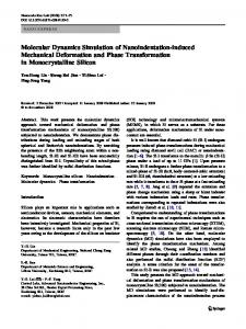
Fig. 7. Analysis of the slowest modes extracted from MD simulations (run MD-1). (a) Trajectory along the first principal axis (or LSV), (b) histogram of the motion along the first LSV, (c) histogram along the second LSV, and (d) trajectory projected onto the first two LSVs.
the most severely contrained residues of tendamistat, along with the strand II residue Asn25. Time Evolution of Molecular Coordinates in the Slowest Modes We now focus on the detailed mechanisms of motions driven by the slowest modes. Insofar as the ms fluctuations are concerned all three theoretical approaches yield similar results, but a number of observations signal the inadequacy of the GNM in the slowest end of the spectrum. To elucidate this point, we examined in detail the mechanisms of the slowest modes operating in runs MD-1 and MD-2. An important observation is that the two MD runs do not exhibit the same type of dominant mechanism of motion in their slowest modes. It is worth mentioning that even the ms fluctuations (of individual residues) that were reconstructed on the basis of the slowest few modes in the two runs were quite different, but only their average (shown in Figure 4 by the bold, dotted curve) were in satisfactory agreement with analytical results. Consistent with this observation the detailed conformational motions undergone in the runs MD-1 and MD-2 were different, when the trajectories along the singular axes were observed. Figure 7a displays the trajectory along the first PA (or first LSV) determined in the run MD-1. One can see unambiguously that the molecule undergoes sharp conformational transitions, indicative of jumps between two or three isomeric states, in agreement with previous observations for other proteins.5,47 Therefore distinct energy wells separated by energy barriers are visited. This type of
motions are certainly non-Gaussian, and GNM cannot describe these. Figure 7d displays the trajectory projected onto the first two LSVs, and Figure 7b and c describe the histograms associated with the motions along the first and second LSVs, respectively. The bimodal probability distribution observed in Part b is consistent with Part a. The motion along the second LSV, on the other hand, obeys a unimodal, but still non-Gaussian, distribution. Part d indicates the possible occurrence of three distinct conformational states visited throughout the run MD-1, although these cannot be distinguished by projecting the trajectory onto the first two LSVs. Snapshots taken at particular states revealed that the conformational jumps essentially consist of a rotational isomerization of one or more bonds at the N-terminal segment, and a rotational motion of the loops connecting strands I-II, and strands IV-V. A similar analysis performed for MD-2, on the other hand, yielded again a bimodal distribution in the slowest mode, although the transitions were not as sharp and as frequent as those in Figure 7. A more collective conformational rearrangement, involving larger scale cooperative fluctuations of the loops was observed in this case. Thus, not the same type of conformational motions are observed in the two runs. Yet, in both simulations the motions responsible for the jumps are rather localized, which conform with singly-hierarchical motions, rather than multiply hierarchical.47 In summary, the average quantities from the independent runs (ms fluctuations or cross-correlations), also evaluated with regard to analytical results, can be viewed as the major physically meaningful and statistically reliable results.
522
P. DORUKER ET AL.
CONCLUSION In conclusion, we may state that the analytical approaches and the simulations yield results that are consistent with each other insofar as the ms fluctuation amplitudes of individual residues (or ␣-carbons) and their correlations are concerned. This observation is significant from the point of view that the neglect of nonlinear effects and atomic details such as residue-specific potentials (in the ANM), or even anisotropic effects (in the GNM) do not significantly affect the observed fluctuation spectrum. A fast and reliable estimation of the fluctuation distribution of individual residues in folded proteins can thus be made by applying the GNM approach, the computational time cost of which is of the order of seconds, as opposed to days for MD simulations. The fact that the ms fluctuations are comparable does not imply that other details about the dispersion of modes or mechanism of motion (see below) can also be reliably estimated from the GNM. The present analysis indeed stipulates which properties can, and which cannot, be satisfactorily described by adopting a highly simplified analytical approach. The ANM is introduced here as a new analytical approach in which one of the major deficiencies of the GNM, the neglect of the anisotropy of fluctuations, is removed. This requires about one order of magnitude longer computational time than the GNM, the Kirchhoff matrix being replaced by a 3n ⫻ 3n matrix of force constants that takes account of the directional preferences of individual residues. Yet, the improvement in overall accuracy in comparison to MD results (see Fig. 2c), and the additional information provided about the directional preferences of fluctuations, and not only about their amplitudes, are in favor of its adoption in analyzing biomolecular systems. We might also recall that the computational time cost of the ANM is still at least two orders of magnitude lower than MD simulations. It is worth noting that the present simulations were carried out in vacuum. Previous MD simulations have shown that solvent has two major effects:5 (i) enhancement of small amplitude conformational motions, giving rise to a more structured free energy surface and lowering of energy barriers, and (ii) damping of collective motions which can be approximated by a suitably adjusted friction coefficient.47,54 Inclusion of solvent indeed affects the mechanism of local anharmonic motions, or the occurrence of isomeric transitions in short solvent-exposed chains such as polypeptides.55 However, the mechanisms of dominant motions controlled by the subspace of slowest modes are rather insensitive to solvent.5,47 Additionally, the correlations of internal motions are similar in different environments, as demonstrated by Ichiye and Karplus in their analysis of cross-correlations and co-variances of atomic fluctuations.21 A direct examination of the MD trajectory reconstructed with a subset of dominant (slowest) modes shows that the types of conformational transitions that operate at the slowest modes regime are not necessarily reproduced in independent runs. One apparently needs to perform many
Fig. 8. Schematic representation of an energy well controlling the collective fluctuations in the folded protein. The structured curve is a realistic energy surface, presumably sampled in MD simulations. The solid and dotted curves are the best fitting harmonic (GNM) and anisotropic (ANM) potentials, respectively. Note that the amplitudes of fluctuations near the minimum of the energy minimum (⌬R2) can be satisfactorily described by an approximate (GNM or ANM) potential, while the departure between the curves increases in the case of larger amplitude (⌬R1) fluctuations.
runs,25 and simple analytical analyses such as GNM or ANM or the highly efficient approximate NMA proposed by Hinsen for example,3 before making conclusive statements about the mechanism of the slowest modes. However, the present analysis shows that one can safely make estimates about the size (amplitudes) of motions in the slowest modes, and their correlations, even by adopting coarse-grained analytical models like ANM. Insofar as mean-square quantities such as residue fluctuations or cross-correlations are concerned, GNM and ANM results indeed appear to be as reliable as the MD results, despite their inadequacy for describing the nonlinear motions, or the jumps between isomeric minima. The key point to understand this somewhat controversial and puzzling agreement between the analytical and numerical results probably lies in the proper choice of the force constant ␥ of the analytical approaches. This parameter directly scales the width of fluctuations, and can be optimally selected to reproduce the observed amplitudes of motions. Figure 8 illustrates for example three potential energy wells about the global minima, one comprising multiple microstates or conformational substates,4 separated by small energy barriers— conforming with the single-hierarchical energy surface of Go and coworkers47— and two smooth potentials, harmonic (solid) and anharmonic (dotted). The ms fluctuations within the harmonic well can be construed to equate to those macroscopically observed in the multimeric well, by proper choice of the curvature (i.e., ␥) of the harmonic potential. Inclusion of anisotropic effects can further account for asymmetry of the well. In a number of proteins, including the ␣-amylase inhibitors presently investigated, the energy landscape near the global minimum can probably be approximated by a single well as a first, coarse-grained approach, unless two or more highly distinct conformational substates (or
COOPERATIVE MOTIONS IN PROTEINS
multiply hierarchical energy wells), such as those observed in human lysozyme,47 cAMP-binding protein2 or T4 lysozyme22 are visited under native state conditions. Finally, on the mechanism of the functional motions of the ␣-amylase inhibitor tendamistat, we conclude from both simulations and analytical calculations that the dominant mode of motion is the opposite direction fluctuations of the two groups of strands {I, II, V} and {III, IV, VI}, which form the respective sheets S1 and S2. It is worth noting that the active site residues 18 –20 at the Nterminus of strand II in S1 are strongly correlated with strand V residues 58 – 60, which in turn are subject to strong anticorrelated motions with the S2 strand III residue 34 –37. The latter strand, and in particular its residues 34 –37, plays a central role in mediating the intersheet interactions (see Fig. 6c). This strand is simultaneously engaged in close correlated motions with strand VI and IV, driving the concerted motion of sheet S2. The present correlation analysis thus unravels the path of intramolecular signal transmission, communicating between the core regions and the recognition sites of the ␣-amylase inhibitor tendamistat—a protein representative of a unique three dimensional fold. ACKNOWLEDGMENT Partial support from Bogazici University Research Funds Projects # 99HA501 and 99HA503 are gratefully acknowledged by P.D. and I.B. REFERENCES 1. Horiuchi T,Go N. Projection of Monte Carlo and molecular dynamics trajectories onto the normal mode axes: human lysozyme. Proteins 1991;10:106 –116. 2. Garcia AE, Harman JG. Simulations of CRP:(cAMP)2 in noncrystalline environments show a subunit transition from the open to the closed conformation. Protein Sci 1996;5:62–71. 3. Hinsen K. Analysis of domain motions by approximate normal mode calculations. Proteins 1998;33:417– 429. 4. Frauenfelder H, McMahon B. Dynamics and function of proteins: the search for general concepts. Proc Natl Acad Sci USA 1998;95: 4795– 4797. 5. Kitao A,Go N. Investigating protein dynamics in collective coordinate space. Curr Opin Struct Biol 1999;9:164 –169. 6. Go N, Noguti T, Nishikawa T. Dynamics of a small protein in terms of low-frequency vibrational modes. Proc Natl Acad Sci USA 1983;80:3696 –3700. 7. Karplus M, Kushick JN. Method for estimating the configurational entropy of macromolecules. Macromolecules 1981;14:325– 332. 8. Levitt M, Sander C, Stern PS. Protein normal-mode dynamics: Trypsin inhibitor, crambin, ribonuclease and lysozyme. J Mol Biol 1985;181:423– 447. 9. Brooks B, Karplus M. Normal modes for specific motions of macromolecules: Application to the hinge-bending mode of lysozyme. Proc Natl Acad Sci USA 1985;82:4995– 4999. 10. Sessions RB, Dauber-Osguthorpe P, Osguthorpe DJ. Filtering molecular dynamics trajectories to reveal low-frequency collective motions: phospholipase A2. J Mol Biol 1988;209:617– 633. 11. Dauber-Osguthorpe P, Osguthorpe DJ. Extraction of the energetics of selected types of motion from molecular dynamics trajectories by filtering. Biochemistry 1990;29:8223– 8228. 12. Levitt M. Real-time interactive frequency filtering of molecular dynamics trajectories. J Mol Biol 1991;220:1– 4. 13. Dauber-Osguthorpe P, Osguthorpe DJ. Partitioning the motion in molecular dynamics simulations into characteristic modes of motion. J Comput Chem 1993;14:1259 –1271. 14. Amadei A, Linssen ABM, Berendsen HJC. Essential dynamics of proteins. Proteins 1993;17:412– 425.
523
15. Aalten DMF, Amadei A, Linssen ABM, Eijsink VGH, Vriend G, Berendsen HJC. The essential dynamics of thermolysin: confirmation of the hinge-bending motion and comparison of simulations in vacuum and water. Proteins 1995;22:45–54. 16. Baysal C, Atilgan AR, Erman B, Bahar I. Coupling between different modes in local chain dynamics: a modal correlation analysis. J Chem Soc Faraday Trans 1995;91:2483–2490. 17. Romo TD, Clarage JB, Sorensen DC, Phillips JGN. Automatic identification of discrete substates in proteins: singular value decomposition analysis of time-averaged crystallographic refinements. Proteins 1995;22:311–321. 18. Levy RM, Karplus M. Vibrational approach to the dynamics of an ␣-helix. Biopolymers 1979;18:2465–2495. 19. Levy RM, Perahia D, Karplus M. Molecular dynamics of an ␣-helical polypeptide: temperature dependence and deviation from harmonic behavior. Proc Natl Acad Sci USA 1982;79:1346 – 1350. 20. Levy RM, Karplus M, Kushick J, Perahia D. Evaluation of the configurational entropy for proteins: application to molecular dynamics simulations of an ␣-helix. Macromolecules 1984;17:1370–1374. 21. Ichiye T, Karplus M. Collective motions in proteins: a covariance analysis of atomic fluctuations in molecular dynamics and normal mode simulations. Proteins 1991;11:205–217. 22. de Groot BL, Hayward S, van Aalten DMF, Amadei A. Domain motions in bacteriophage T4 lysozyme: a comparison between molecular dynamics and crystallographic data. Proteins 1998;31: 116 –127. 23. Kitao A, Hirata F, Go N. The effects of solvent on the conformation and the collective motions of a protein: normal mode analysis and molecular dynamics simulations of melittin in water and in vacuum. Chem Phys 1991;158:447– 472. 24. Clarage JB, Romo T, Andrews BK, Pettitt BM, Phillips JGN. A sampling problem in molecular dynamics simulations of macromolecules. Proc Natl Acad Sci USA 1995;92:3288 –3292. 25. Caves LSD, Evanseck JD, Karplus M. Locally accessible conformations of proteins: multiple molecular dynamics simulations of proteins. Protein Sci 1998;7:649 – 666. 26. Bahar I, Atilgan AR, Erman B. Direct evaluation of thermal fluctuations in proteins using a single parameter harmonic potential. Fold Des 1997;2:173–181. 27. Jernigan RL, Bahar I. Structure-derived potentials and protein simulations. Curr Opin Struct Biol 1996;6:195–209. 28. Bahar I, Jernigan RL. Inter-residue potentials in globular proteins and the dominance of highly specific hydrophilic interactions at close separation. J Mol Biol 1997;266:195–214. 29. Tirion MM. Large amplitude elastic motions in proteins from a single-parameter, atomic analysis. Physical Review Letters 1996; 77:1905–1908. 30. Bahar I, Wallquist A, Covell DG, Jernigan RL. Correlation between native state hydrogen exchange and cooperative residue fluctuations from a simple model. Biochemistry 1998;37:1067– 1075. 31. Haliloglu T, Bahar I. Structure-based analysis of protein dynamics near the folded state. Results for hen lysozyme, and comparison with X-ray diffraction and NMR relaxation data. Proteins 1999;37:654 – 667. 32. Bahar I, Erman B, Jernigan RL, Atilgan AR, Covell DG. Collective dynamics of HIV-1 reverse transcriptase: examination of flexibility and enzyme function. J Mol Biol 1999;285:1023–1037. 33. Bahar I, Jernigan RL. Vibrational dynamics of transfer RNAs: comparison of the free and enzyme bound forms. J Mol Biol 1998;281:871– 884. 34. Bahar I, Jernigan RL. Cooperative fluctuations and subunit communication in tryptophan synthase. Biochemistry 1999;38: 3478 –3490. 35. Press WH, Teukolsky SA, Vetterling WT, Flannery BP. Book numerical recipes in fortran. The art of scientific computing. Cambridge: Cambridge University Press; 1992. 963 p. 36. Kuriyan J, Petsko GA, Levy RM, Karplus M. Effect of anisotropy and anharmonicity on protein crystallographic refinement. An evaluation by molecular dynamics. J Mol Biol 1986;190:227–254. 37. Hubbard TJP, Ailey B, Brenner SE, Murzin AG, Chothia C. SCOP: a structural classification of proteins database. Nucleic Acids Res 1999;27:254 –256. 38. Hayward S, Kitao A, Go N. Harmonicity and anharmonic aspects in the dynamics of BPTI: a normal mode analysis and principal component analysis. Protein Sci 1994;3:936 –943.
524
P. DORUKER ET AL.
39. Pflugrath JW, Wiegand G, Huber R,Ve´rtesy L. Crystal structure determination, refinement and the molecular model of the ␣-amylase inhibitor Hoe-467A. J Mol Biol 1986;189:383–386. 40. Kline AD, Braun W, Wu¨thrich K. Determination of the complete three-dimensional structure of the ␣-amylase inhibitor tendamistat in aqueous solution by nuclear magnetic resonance and distance geometry. J Mol Biol 1988;204:675–724. 41. Billeter M, Schaumann T, Braun W, Wu¨thrich K. Restrained energy refinement with two different algorithms and force fields of the structure of the ␣-amylase inhibitor tendamistat determined by NMR solution. Biopolymers 1990;29:695–706. 42. van Gunsteren WF, Berendsen HJC. Groningen molecular simulation (GROMOS) library manual. 1987. Biomos, Nijenborgh 4, 9747 AG Groningen, The Netherlands. 43. Ryckaert J-P, Ciccotti G, Berendsen HJC. Numerical integration of cartesian equations of motion of a system with constraints: molecular dynamics of n-alkanes. J Comput Phys 1977;23:327– 341. 44. van Gunsteren WF, Berendsen HJC. Computer simulation of molecular dynamics: methodology, applications, and perspectives in chemistry. Angew Chem Int Ed Engl 1990;29:992–1023. 45. Bernstein FC, Koetzle TF, Williams GJB, et al. The protein data bank: a computer based Archival file for macromolecular structures. J Mol Biol 1977;112:535–542. 46. Berendsen HJC, Postma JPM, van Gunsteren WF, DiNola A, Haak JR. Molecular dynamics with coupling to an external bath. J Chem Phys 1984;81:3684 –3690.
47. Kitao A, Hayward S, Go N. Energy landscape of a native protein: jumping-among-minima model. Proteins 1998;33:496 –517. 48. Demirel MC, Bahar I, Atilgan AR. Predicting the ensemble of unfolding pathways for proteins: an updated incremental Lagrangian model. Biophysical J 1999;76:A176. 49. Sternberg MJE, Grace DEP, Grace DC. Dynamic information from protein crystallography. An analysis of temperature factors from refinement of the hen egg-white lysozyme structure. J Mol Biol 1979;130:231–253. 50. Artmiyuk PJ, Blake CCF, Grace DEP, Oatley SJ, Phillips DC, Sternberg MJE. Crystallographic studies of the dynamic properties of lysozyme. Nature (London) 1979;280:563–568. 51. Frauenfelder H, Petsko GA, Tsernoglou D. Temperature-dependent X-ray difffraction as a probe of protein structural dynamics. Nature 1979;280:558 –563. 52. Bahar I, Atilgan AR, Demirel MC, Erman B. Vibrational dynamics of folded proteins. Significance of slow and fast modes in relation to function and stability. Phys Rev Lett 1998;80:2733–2736. 53. de la Cruz X, Mark AE, Tormo J, Fita I, van Gunsteren WF. Investigation of shape variations in the antibody binding site by molecular dynamics computer simulation. J Mol Biol 1994;236: 1186 –1195. 54. Hayward S, Kitao A, Hirata F, Go N. Effect of solvent on collective motions in globular protein. J Mol Biol 1993;234:1207–1217. 55. Doruker P, Bahar I. Role of water on unfolding kinetics of polypeptides studied by molecular dynamics simulations. Biophys J 1997;7:2445–2456.