(BBL) in Lake Kinneret, Israel, a large lake that experiences strong thermal stratification and wind forcing events. Microstructure data were used to derive the ...
� Springer 2006
Hydrobiologia (2006) 568:217–233 DOI 10.1007/s10750-006-0111-6
Primary Research Paper
Dynamics of the benthic boundary layer in a strongly forced stratified lake Clelia Luisa Marti1,2,* & Jo¨rg Imberger1 1
Centre for Water Research, The University of Western Australia, 6009 Crawley, WA, Australia Facultad de Ingenierı´a y Ciencias Hı´dricas, Universidad Nacional del Litoral, Ciudad Universitaria, Ruta Nacional No 168 – Km. 472,4, C.C. 217, 3000 Santa Fe, Argentina (*Author for correspondence: E-mail: cmarti@fich1.unl.edu.ar) 2
Received 5 September 2005; in revised form 5 February 2006; accepted 26 February 2006; published online 15 May 2006
Key words: benthic boundary layer, stratified lake, gravitational flow, internal waves
Abstract Field data and the three-dimensional (3D) Estuary and Lake Computer Model (ELCOM) were used to investigate the impact of periodic forcing on the structure and dynamics of the benthic boundary layer (BBL) in Lake Kinneret, Israel, a large lake that experiences strong thermal stratification and wind forcing events. Microstructure data were used to derive the thickness of the BBL and to describe the mean turbulent properties within the BBL. Time series temperature data from thermistor chains were used to characterize the thermal structure of the lake and the basin-scale internal wave field in the lake that was shown to force the turbulent field in the BBL. A clear connection between the dynamics of the BBL and the large-scale features of the flow is presented. The time history of the thickness of the BBL, the mixing in the BBL and the resulting cross-shore flux were shown to vary with the phase of the basin-scale internal wave field. Detailed comparison of simulation results with field data revealed that the model captured well the lake hydrodynamics and the spatial and temporal evolution of energetics of the BBL. Together, field data and numerical modelling provided a clear characterization of the dynamics of the turbulent BBL and its central role in setting up a boundary layer mass flux up the slope from the lake bottom to the height of the metalimnion. Both the turbulent environment in the BBL and the mass flux are of great importance for the ecological processessing of material in a lake.
Introduction The benthic boundary layer (hereafter abbreviated as BBL) may be defined as the fluid layer, adjacent to the bottom, in which the bottom shear and internal wave breaking causes active mixing leading to strong dissipation of turbulent kinetic energy and a uniformity of temperature and other water column properties. It is a layer in which many interrelated physical, geochemical and biological processes actively take place (Bowden, 1978; Grant & Madsen, 1986). Although those interrelated processes are complex and many of them are still not well understood, they are believed to have a great impact on the water quality
of the overlying water (Nishri et al., 2000; Boudreau & Jørgensen, 2001; Turnewitsch & Springer, 2001; Turnewitsch & Graf, 2003). The exchange of momentum, heat, solutes (such as oxygen), particles, and organisms between the water column and sediment takes place within this layer (Richards, 1990). The BBL is the endpoint of sedimenting material that stimulates high metabolic rates for microbial populations both in the near bottom waters and in the superficial sediment layers (Poremba & Hoppe, 1995; Boetius et al., 1996). Furthermore, the redissolution and subsequent transport of solutes supply primary producers with nutrients and can affect the stability of the water column by chemical stratification (Wu¨est & Gloor,
218 1998). Thus, the BBL acts as a turbulent mixed reactor separating the water column above from the very thin, often nutrient rich, sediment interface and so controlling the benthic–pelagic coupling (Baccini, 1985; Fre´chette et al., 1989; Shimeta et al., 2001). The existence of BBL has been reported for a variety of marine and freshwater environments. The BBL in oceans and lakes is usually actively turbulent (Thorpe, 1988; Wu¨est & Lorke, 2003) and identified as a layer of constant temperature, density or salinity directly above the bottom. In the ocean, BBL’s generally exhibits a thickness of circa 100 m (e.g., Armi & Millard, 1976; Ivey, 1987; Beaulieu & Baldwin, 1998), but in strongly stratified water systems, the thickness can often be only a few metres or even less (e.g., Imberger & Ivey, 1993; Gloor et al., 1994; Stips et al., 1998; Gloor et al., 2000; Wu¨est & Lorke, 2003; Lemckert et al., 2004; Hondzo & Haider, 2004). The thickness of the BBL has been found to vary dramatically over sloping boundaries within both oceans and lakes (Lentz & Trowbridge, 1991; Gloor et al., 1994; Stips et al., 1998; Gloor et al., 2000). Stips et al., (1998) found that within shallow seas, the mixing processes responsible for the layer thickness were not produced locally, but most probably due to turbulence patches being advected into the region. In Lake Alpnach, Gloor et al. (2000) showed that short-term changes in the BBL thickness on the sloping boundaries were associated with advection induced by basin-scale internal waves. By contrast repeated intrusions of boundary mixed water into the lake interior possibly explained the rapid decay in BBL thickness. Recent studies have emphasized the importance of the BBL for the overall energy dissipation in aquatic systems and suggest that the BBL is the major energy sink for basin-scale currents due to bottom friction and breaking of high frequency waves as they shoal upon sloping boundaries at the depth of the metalimnion (Boegman et al., 2003; Yeates & Imberger, 2004). Field results have shown that the level of turbulence near basin boundaries and topographic features can be several orders of magnitude higher than turbulence offshore (Van Haren et al., 1994; Goudsmit et al., 1997; Imberger, 1998; MacIntyre et al., 1999; Gloor et al., 2000; Yeates & Imberger, 2004).
The large-scale currents, which are very often periodic, are predominantly produced by basinscale internal waves in enclosed stratified water bodies (Gloor et al., 2000; Antenucci et al., 2000; Lorke et al., 2002). The near bottom speeds are usually in the range of �2 to �10 cm s)1 (Lemmin, 1987; Gloor et al., 1994; Ravens et al., 2000) and may trigger resuspension, mixing and transport of particles and nutrients within the BBL (Gloor et al., 1994; Pierson & Weyhenmeyer, 1994; Shteinman et al., 1997). Also the key processes for sediment/water exchange, molecular diffusion, porewater convection/advection and bioturbation are all dependent on the horizontal currents in the BBL (Huettel et al., 2003). The resulting wellmixed water may then be transported into the lake interior as intrusions along the isopycnals (Thorpe, 1998; McPhee-Shaw & Kunze, 2002). Consequently, it may be expected that the periodicity and magnitude of basin-scale currents, and the resulting periodic BBL turbulence, affect both the vertical and lateral transport of solutes and resuspended particles. Proper characterization of the BBL dynamics and fluxes of water within and out of the BBL are thus required for water quality modelling. There has been a large body of theoretical work, suggesting that enhanced mixing in the BBL leads to an adjustment of the local density field which in turn drives an upslope gravitational updraft in the BBL (Garret, 1990; Imberger & Ivey, 1993; Wu¨est et al., 1996) and feeding intrusions propagating into the interior of the water body; providing a flux path between the hypolimnion and the epilimnion (Munk, 1966; Ivey & Corcos, 1982). So far there have not been any published direct current or indirect tracer measurements that unequivocally verify whether a BBL updraft actually exists; such a flux path is suggested only by theoretical models (Imberger & Ivey, 1993) and circumstantial evidence from transport measurements of tracers (Wu¨est et al., 1996). Nor is it known whether such transport is the result of gravitational adjustments or non-linear wave dynamics. In this paper, the temporal ‘‘diurnal’’ and spatial dynamic behaviour of the currents and turbulence structure of the BBL in a large stratified lake is investigated by combining measurements of the background flow conditions with measurements
219 of properties of the turbulence. This paper is focused particularly on the water mass transport within the BBL and the mechanisms responsible for such transport. The experimental work in this paper was carried out in Lake Kinneret, Israel, during 1999 and 2001. Data presented in this paper were collected using thermistor chains and a microstructure profiler capable of measuring temperature, temperature gradient, conductivity and velocity. In addition, numerical simulations were conducted using the 3D hydrodynamic model ELCOM, with a new mixing model, to document the spatial and temporal variability of the BBL characteristics.
Methods
Tabha
12 T1 T2 Tb 32
T3 Tf 42
T4 53
T5 52
Tiberias
Study site Lake Kinneret (Fig. 1) lies approximately 209 m below the mean sea level in the northern part of the Great Afro-Syrian Rift (Israel). It measures 22 km from north to south and 12 km form east to west, has a surface area of about 168 km2, a mean depth of 24 m and a maximum depth of 43 m. Lake Kinneret’s bathymetry slopes steeply along the eastern shore and gradually along the northern, western and southern shores. From early spring (April) until late autumn (December), the water column exhibits a stable density stratification with epilimnetic water temperatures reaching 30 �C in the peak of summer. Strong westerly winds (wind speed �12 m s)1) during summer afternoons (Serruya, 1975) excite a broadband of basin-scale internal waves of various horizontal and vertical modes. In their analysis of thermistor chain data from 1997 and 1998, Antenucci et al. (2000) identified a 24 h period, vertical-mode-one Kelvin (cyclonic) wave as the dominant response to the wind forcing. Verticalmode-one, -two and -three Poincare´ (anticyclonic) waves were also observed with periods of 12, 20 and 20 h, respectively. Lemckert et al. (2004) documented the existence of a well-developed BBL, evolving with the vertical-mode-one seiche and capped by the stratification of the overlying water column, the interpretations were all in terms of a vertical one-dimensional mixing layer (at seasonal time scale) and little direct information
1999 2001
0
1000 2000
Metres
Figure 1. Bathymetric map of Lake Kinneret with sampling stations. Contour intervals are given in metres below the mean sea level. The locations of the thermistor chain stations are marked with a T; the numbers and letters correspond to sampling stations.
was presented on the induced upslope or downslope fluxes of water. Field experiment Data used in this investigation were collected during two field experiments conducted in Lake Kinneret. The first study was performed from 14 June to 02 July, 1999 (days 165 and 183), while the second was performed from 19 June to 01 July, 2001 (days 169 and 182); both covering periods where natural resonance of wind and internal waves caused large internal wave amplitudes (Antenucci & Imberger, 2003). Details of the
220 instrument deployments relevant to this study are presented in Table 1 and Figure 1. Temperature data were collected using thermistor chain moorings located at five stations (labelled T1, T2, T3, T4 and T5 in Figure 1) aligned with the principal axis of the dominant wind direction during 1999 and at Stations Tb and Tf during 2001, which were placed at the same location of Stations T2 and T3, respectively. Each chain consisted of a series of fast response thermistors, with accuracies of 0.01 �C, vertically spaced at 1 m intervals in the metalimnion and up to 5 m intervals in the epilimnion and hypolimnion during 1999 and every 0.75 m during 2001. All stations were equipped with wind speed and direction sensors mounted 2.4 m above the water. All data were recorded at 10 s intervals and were telemetered to a shore station. Time series of isotherm displacements were determined from linear interpolation of temperature records. Microstructure profiles of temperature, temperature gradient, conductivity, and three components of velocity were measured using the Portable Flux Profiler (PFP; Imberger & Head, 1994). Profiles were taken close to Stations T1 and T2 and a transect, cycling from Station T5 through
to Station T12 during 1999, and close to Stations Tb and Tf during 2001, at various times in order to document the temporal evolution of the turbulent structure of the BBL during periods of maximum internal wave amplitudes. The total number of PFP profiles taken during 1999 and 2001 field experiments were 259 and 360, respectively. The PFP has two combined four-electrode temperature and conductivity sensors (0.001 �C and 0.0004 S m)1 resolution respectively) mounted in the front of the probe between a pair of orthogonal two-component forward scatter laser Doppler velocimeters (0.001 m s)1 resolution). Profiling vertically through the water column at a speed of �0.1 m s)1 and a sampling frequency of 100 Hz, the PFP resolved the water column structure with vertical scales as small as 1 mm. The PFP data processing techniques used in this paper follow those used by Saggio & Imberger (2001) and are only briefly outlined here. After filtering and response time correction (Fozdar et al., 1985), the temperature profiles were divided into statistically stationary segments by use of the method of Imberger & Ivey (1991) before performing spectral analysis. In most profiles, the BBL regions, in their entirety, were statistically
Table 1. Details of instrument deployments in 1999 and 2001 experiments (TC=thermistor chain) Sta.
Instrument
Year
Period (Day number)
Depth range (m)
T12
PFP
1999
180
10
T1
TC
1999
From 171 to 183
15
T1
PFP
1999
173/174/178/179/180
15
T2
TC
1999
From 167 to 183
22
T2 Tb
PFP TC
1999 2001
173/174/178/179/180 From 166 to 182
22 22
Tb
PFP
2001
175
22
32
PFP
1999
180
25
T3
TC
1999
From 165 to 181
29
T3
PFP
1999
180
29
Tf
TC
2001
From 166 to 182
29
Tf
PFP
2001
171/172/175/176/179
29
42 T4
PFP TC
1999 1999
180 From 168 to 181
36 39
T4
PFP
1999
180
39
53
PFP
1999
180
40
52
PFP
1999
180
34
T5
TC
1999
From 166 to 182
22
T5
PFP
1999
180
22
221 stationary and therefore they could be characterised as one event. The upper limits of these layers were marked by sharp changes in temperature gradient as the near homogeneous BBL water interacted with the stratified interior lake water. In this study, following previous works (Lentz & Trowbridge, 1991; Houghton, 1995) the BBL was defined as the region near the bottom where the observed temperature was within some value DT of the observation closest to the bottom and the turbulence was statistically stationary; DT was chosen to be 0.1 �C, which coincided with the sharp transition in the temperature profile. Rates of dissipation of turbulent kinetic energy were calculated for each data segment using a Batchelor curve-fitting technique described in Luketina & Imberger (2001). This permitted the dissipation to be estimated down to 10)10 with an error of ER þ Ee (i.e., DEM ¼ EA � ER � Ee ; DEM > 0); the mixing fraction being determined by the ratio of the mixing time scale (Tm) to the time step (Dt). The energy remaining after a mixing event was reduced to allow for dissipation between time steps given by Ee ¼ ð0:5 CE DtÞ ðEA =DzÞ3=2 , with CE=1.15 (Spiegel et al., 1986), Dz the vertical distance between vertically adjacent cell centres and Dt the computational time step. With this scheme, a surface mixed layer ‘grew’ by discrete homogenization of the grid cells; the same algorithm was applied down through the water column below the diurnal thermocline, thus allowing for mixed patches within the water column. This version of the model was, however, grid dependent and also did not account for the TKE introduced by the bottom drag. The version of the model used in this study incorporates a modified mixing model that corrected these defects. The changes included first, a parameterization of energy introduced by bottom stirring
222 induced by the bottom drag (EB) using an analogue of the wind-mixed surface layer counterpart. Second, the mixing fraction was calculated from a turbulent diffusive coefficient, obtained direct the field measurements and based on the gradient Richardson number parameterization. Third, a scale correction to capture the effect of the vertical grid size on the computation of the gradient Richardson number was included to make the algorithm grid independent. This new mixing algorithm has been described in detail by Simanjuntak et al. (2006; submitted). However, for convenience, a brief description is presented here. Energy production by the bottom drag The benthic energy (EB) from the bottom friction was parameterized as Ck u3�bott , with Ck=2.2 (Sherman et al., 1978), and u2�bott ¼ Cd U2bott the bottom shear velocity. Here Ubott is the magnitude of the horizontal velocity in computational cells adjacent to the bottom and Cd is a bottom drag coefficient (as a user input). The downward direction of the mixing model means that EB moves upward one cell only for every time step and is reduced by the dissipation before it moves up one cell; sweeping upward did not change the results significantly. Diffusivity closure The new diffusivity closure is based on the microstructure measurements in Lake Kinneret by Saggio and Imberger (2001) and Yeates and Imberger (2004) and consists of 4 dynamical regimes. First, a neutral water column regime where the vertical diffusion coefficient (jq ) is given by a Smagorinski type parameterization depending only on the shear and the vertical grid size. Second, a stratified region where the vertical diffusion coefficient is given by jq 0:15 ¼ � Ri j
ð1Þ
where the compound Richardson number (Ri*) is defined as:
Ri� ¼ �
DU Dz
�2
N2 TKE� Dz�3 þ Fm � 0:5F2m
ð2Þ
where N2 is the buoyancy frequency, DU the horizontal velocity difference between vertically adjacent grid cells, Dz the vertical distance between vertically adjacent cell centres, Fm the mixing fraction, and TKE� ¼ EW þ EB þ EC þ EM the contribution from sources other than the mean shear. The mixing fraction was determined from the relationship: Fm ¼
Dz2 jq Dt
ð3Þ
The stratified region consists of two regimes: an energetic regime (Ri� 5�10)3 rad2 s)2), and dissipation values generally more variable and ranged between 10)10 m2 s)3 and 10)5 m2 s)3.
Similar observations were made by Saggio & Imberger (2001). In some cases, current speeds between 0.15 and 0.20 m s)1 were observed in the metalimnion (Figs. 3j, n and 4f). The hypolimnion, depending on the location, extended from 12–18 m deep to 2–8 m above the bottom sediments and was characterized by weak stratification, temperatures between 17 and 18 �C and dissipation values that seldom-exceeded 10)8 m2 s)3. Hypolimnetic current speeds were generally less than 0.10 m s)1. A mixed BBL or constant temperature layer is clearly visible in the profiles in Figures 3a, e, i, m and 4a, e (shaded areas) and the thickness of this mixed BBL changed in both time and space. Dissipation values in the BBL ranged from 10)9 m2 s)3 at the top of the BBL to 10)5 m2 s)3 near the sediment boundary. In most cases, the top of the mixed BBL was also characterized by a rapid decrease in the fluctuating velocity component u¢, indicating that the thickness of both the mixed and mixing BBL coincided (Figs. 3k and 4c, g (shaded areas)), however at other times the two diverged (Figs. 3c, o and 4c (shaded areas)). The surface layer and BBL regions were characterized by strong u¢ signal and Richardson numbers (Ri) consistently below the critical value of 0.25. The u¢ signal rapidly decreased at the top of the BBL and at the bottom of the surface layer; the v and w fluctuations (not shown) showed similar behaviour. Interestingly, in most cases the mixed BBL thickness coincided with the vertical extent of the low Richardson number region near the bottom. In contrast, the motion in the metalimnion was characterized by high Richardson numbers. However, there were regions in the metalimnion with strong u¢ signals and Ri