Nov 26, 2013 - arXiv:1311.6825v1 [hep-ph] 26 Nov 2013. Page 2. 2 born13-procs printed on November 28, 2013. Figure 1. Thermal behaviour of the model ...
Dynamics of the chiral phase transition∗
arXiv:1311.6825v1 [hep-ph] 26 Nov 2013
H. van Hees1,2 , C. Wesp1 , A. Meistrenko1 and C. Greiner1 1
2
Institut f¨ ur Theoretische Physik, Goethe-Universit¨at Frankfurt, Max-von-Laue-Straße 1, D-60438 Frankfurt, Germany Frankfurt Institute for Advanced Studies, Ruth-Moufang-Straße 1, D-60438 Frankfurt, Germany
The intention of this study is the search for signatures of the chiral phase transition in heavy-ion collisions. To investigate the impact of fluctuations, e.g., of the baryon number, at the transition or at a critical point, the linear sigma model is treated in a dynamical (3+1)-dimensional numerical simulation. Chiral fields are approximated as classical mean fields, and quarks are described as quasi particles in a Vlasov equation. Additional dynamics is implemented by quark-quark and quark-sigma-field interactions. For a consistent description of field-particle interactions, a new Monte-Carlo-Langevin-like formalism has been developed and is discussed. PACS numbers: PACS numbers come here
1. Introduction In this proceeding we will present our work on the linear σ-model off thermal equilibrium. Section 2 describes the physical model with the numerical implementation described in section 3. Consistency tests and results are discussed in section 4 in which we also discuss difficulties implicated by only including elastic and mean-field interactions in such a model. In section 5 we will relate to this class of problems and discuss our new method to allow hard and scattering-like interactions between particles and classical fields. 2. Linear σ-model For our numerical studies we use the effective O(4)-linear sigma model [1, 2], which is motivated by the chiral symmetry of QCD. It is a model with constituent quarks and anti-quarks, coupled to the chiral fields φ ∈ ∗
XXXI Max Born Symposium and HIC for FAIR Workshop
(1)
2
born13-procs
printed on November 28, 2013
Figure 1. Thermal behaviour of the model when initialised in equilibrium. Depending on the coupling strength, the order of the phase transition changes.
R4 . By spontaneous and explicit symmetry breaking, the chiral fields are decomposed into the pionic fields ~π and a massive field σ, acting as an order parameter. The Lagrangian reads � � 1 L = ψ¯ i∂/ −g (σ + i~π · ~τ γ5 ) ψ − (∂µ σ∂ µ σ + ∂µ~π ∂ µ~π ) − U (σ, ~π ) (1) 2 with the chiral potential �2 λ2 2 σ + ~π 2 − ν 2 + U0 (fπ , mπ , σ). (2) 4 Quarks are dynamically coupled to the meson mean fields via their dispersion relation: U (σ, ~π ) =
Eq2 = p2 + m2q (x, t), � � m2q (x, t) = g 2 σ 2 (x, t) + π 2 (x, t) ,
(3) (4)
leading to a position and time dependent mass term for the quarks. The model parameters are chosen to fit the pion mass, mπ = 138 MeV, and the vacuum expectation value of the order parameter hσi0 = fπ = 93 MeV in the vacuum. With an interaction coupling of g = 3-6, the constituentquark mass can be adjusted to mq ≈ 330 MeV. Depending on U0 , chiral symmetry can be explicitly broken leading to a non-vanishing pion mass, mπ . These lead to the parameters λ2 = 20, g = 3-6, U0 = � adjustments 4 2 2 2 mπ / 4λ − fπ mπ , and ν 2 = fπ2 − m2π /λ2 . Figure 1 shows the thermal behaviour of the model when it is initialised in a state of kinetic and chemical equilibrium.
born13-procs
printed on November 28, 2013
3
Quark Energy Distribution 0
0.5
1
1.5
3.5
3.5
0.0 fm/c 0.5 fm/c 2.0 fm/c 5.0 fm/c 10 fm/c 20 fm/c
3
2.5
T= 150 MeV T= 140 MeV T= 123 MeV T = 89 MeV T = 80 MeV T = 80 MeV
2
3
2.5
2
1.5
1.5
1
1
0.5
0.5
0
0.5
1
1.5
E [GeV]
Figure 2. Thermal cooling of the quarks via interaction with a heat-bath.
3. Numerical implementation For the numerical implementation we treat the meson fields on the meanfield level and the quarks as particles in a Vlasov equation for their phasespace distribution function f (t, r, p), augmented by dissipation and particle production, �
� p ∂t + · ∇r − ∇r E(t, r, p) · ∇p f (t, r, p) E(t, r, p) +‘Dissipation’ + Particle production = 0.
(5)
The phase-space distribution function for the quarks is treated in a MonteCarlo test-particle description, f (t, r, p) =
1 X (3) δ [r − ri (t)] δ (3) [p − pi (t)] . Ntest
(6)
i
The mean-field equations for the meson fields, � ¯ − fπ m2 ∂µ ∂ µ σ + λ2 σ 2 + ~π 2 − ν 2 σ + ghψψi π +‘Dissipation’ + Particle prod. = 0 are solved on a 3D grid using the leap-frog algorithm.
(7)
4
born13-procs
printed on November 28, 2013
Figure 3. Expansion of a droplet initial condition. The particle densities and momenta are sampled according to a Woods-Saxon potential.
3.1. Quark Interactions So far, the quarks are coupled to the chiral mean fields only via the Vlasov term. To add additional dynamics and interactions, we implement a collision term for the quasi-particles. This method is equivalent to the approach used in the BAMPS model [3]. The quark’s position space is divided into grid cells ∆3 x, allowing all particles within a cell to interact. The interaction probability is given by P22 =
s σ22 ∆t , E1 E2 Ntest ∆3 x
(8)
with σ22 denoting an isotropic and constant cross section. Additionally we want to be able to cool down or to heat up the system. Implementing a virtual heat bath, the quasi-particles can interact with thermal particles sampled from a heat bath, allowing the particles to statistically gain or lose energy. Figure 2 shows the change of the system’s temperature due to kinetic interactions of the quarks with a virtual heat bath. In this scenario, the quarks are cooled from T = 150 MeV to T = 80 MeV. 4. Test Cases and Results Several test cases and scenarios have been simulated. In basic scenarios, we have checked for numerical stability, energy conservation, vacuum properties and have compared the temperature dependent equilibrium properties with values from the literature [4]. Figure 3 shows a thermal-droplets scenario. The system is initialised with a thermal Woods-Saxon potential to resemble a hot and dense fireball. Then the system cools down by expansion and shows shell-like structures of the quark distribution and the chiral fields.
born13-procs
printed on November 28, 2013
5
1 Loop Scalar Density 0.09 0.008
0.11
0.12
0.13
0.14
0.15
0.16
0.17
0.18 0.008
Equilibrium g = 3.30 g = 3.63 g = 5.50
0.007
0.006 qq - Scalar Density [GeV3 ]
0.1
0.007
0.006
Constant quark density: g = 3.30 g = 3.63 g = 5.50
0.005
0.005
0.004
0.004
0.003
0.003
0.002
0.002
0.001
0.001
0
0 90
100
110
120
130 140 T [MeV]
150
160
170
180
Figure 4. Comparison of the scalar density, hψψi, in case of thermal and chemical equilibrium (solid line) with the case of an expanding medium without chemical processes. Both simulated systems are in a box and cooled down by interactions with the heat bath. Without the chemical processes, no phase transition occurs, and the system is trapped in the chiral-symmetry restored phase.
Two interesting scenarios are shown in figure 4. In both scenarios, an initially equilibrated system is simulated in a box. By interactions of the quarks with a thermal heat bath, the system’s temperature can be adjusted. The system in full chemical and thermal equilibrium shows a phase transition at a given temperature. Due to the lack of chemical processes, the second system does not show a phase-transition behaviour any more. In both cases the system’s thermal energy changes but without a change in the quark density, the system is trapped in its initial chiral state. Extending the current model with chemical processes is not trivial if total energy should be conserved. The Yukawa interaction allows for a ψψ → σ reaction. However, this process is not a continuous one but acts simultaneously on the field and the particles. While creating and annihilating the particles is a simple numerical exercise, the quasi instantaneous particle-like interaction with the filed is completely undefined. This problem is discussed in the following section.
6
born13-procs
printed on November 28, 2013
5. Particle-wave interaction In the linear sigma model, particles and chiral fields are coupled via the Yukawa like coupling. In our model, this is implemented via the interaction potential in the Vlasov equation (5). The gradient of the field energy acts as a continuous force on the quarks, describing the interaction between the quarks and the mean fields. This interaction changes the quarks’ momenta but lacks dissipation and entropy production and thus can not drive the system to thermal equilibrium. By including binary collisions (see section 3.1) between the quarks, a kinetic thermalisation of the quarks can be achieved, but so far the model lacks thermal and chemical equilibration among the quarks and meson-mean fields, i.e., collective coherent oscillations of the fields are not damped by the quark bath. In other models [4, 5, 6], the equations of motion are extended with a Langevin-like coupling. For example, the σ field is damped with a dissipative term, and additionally a noise term is added. This allows for an effective thermalisation of the meson-mean fields, but the quarks are treated as a large (thermalised) reservoir, and the energy and momentum transfer from the mean fields to the medium is neglected. The friction term in the Langevin-mean-field equation thus leads to a continuous rescaling of the quark energy, violating energy (and momentum) conservation. To solve this problem we follow an ansatz motivated from kinetic theory. Thus we treat the dissipation and noise of the mean fields as an interaction between the quarks and the mean fields in a “collision like” way, treating the interactions as local in time and with a non-continuous energy-momentum transfer.
5.1. Energy transfer between fields and particles The main problem of this approach is to find an effective way to simulate such collision-like interactions between particles and mean fields since the here used classical transport approach lacks a clear interpretation in a kind of “field-particle duality”. Here we use energy and momentum as a common feature of particles and fields and describe their exchange between particles and mean fields in a pragmatic stochastical way. The expressions for the energy of the mean fields follow from the Lagrangian making use of Noether’s theorem applied to the symmetry under space-time translations, leading to the total energy and momentum of the
born13-procs
printed on November 28, 2013
7
field in a spatial volume V , Z E=
3
Z
d x �(x) = ZV
P = V
d3 x Π(x) =
ZV
�
� 1 ˙2 1 ~ 2 d x φ + (∇φ) + U (φ) 2 2 3
V
~ d3 xφ˙ ∇φ.
(9) (10)
To simulate a chemical annihilation of a quark pair, ψ + ψ¯ → φˆ → φ
(11)
we treat the annihilation as a 2 → 1 reaction of the ψ ψ¯ pair to an interˆ which is defined via its four-momentum. We map this mediate particle φ, four-momentum to an energy and momentum transfer ∆E and ∆P to the meson-mean field, φ(x, t). For a given field φ(t), the equations of motion describe the propagation of the field to a later time φ(t) → φ(t + δt). Besides this normal propagation, we allow the field to suffer small kicks δφ(xk , tk ) at given discrete times tk and positions xk . These kicks can both increase or decrease the field’s energy, given by a variable ∆E(t). The change of the field δφ is constrained by the energy-momentum equations (9) and (10): ∆E(tk ) = E [φ(x, tk ) + δφ(x, tk )] − E [φ(x, tk )] , ∆P (tk ) = P (φ(x, tk ) + δφ(x, tk )) − P (φ(x, tk )) .
(12) (13)
In the general case, we can not find an inverse of this energy-momentum functional, and we have to solve equations 12 and 13. In the (1+0)-dimensional case, a closed solution can be found, if the potential V (x) can be inverted. In the multi-dimensional case, there is no unique solution to (1213) anymore, and the field increment δφ has to be parameterised. To obtain mathematical stability in the equations of motion, the parameterisation has to be continuous, non-pointlike and must have the same parametrical degrees of freedom as equations (12) and (13) (two for the one-dimensional case and four for the three-dimensional case). We have chosen a travelling Gaussian wave packet as a parameterisation. Even though it is numerically more challenging, we have two advantages compared to the above described Langevin approaches: a discrete control of the field energy change ∆E(tk ) allows for the microcanonical description of a field-particle coupling without the need of an uncontrolled heat bath. Secondly instead of a continuous and deterministic φ˙ term, we can model a discrete and Monte-Carlo like energy transfer ∆E(t).
8
born13-procs
printed on November 28, 2013
To test our method, we were inspired by [7] and have investigated a simple but well understood model, the classical damped harmonic oscillator coupled to a Langevin equation ∂ ∂2 φ(t) + γ φ(t) + φ(t) = κξ(t) ∂t2 ∂t with the usual dissipation-fluctuation relation for the noise term, r 2γT κ= dt
(14)
(15)
These equations of motion describe a damped harmonic oscillator, which is driven by a random force, where ξ(t) is a Gaussian random variable (“white noise”) which can increase or decrease the energy of the system by ’kicking’ the oscillator. On average, the oscillator will show a Gaussian position distribution and an exponential energy distribution ∝ exp(−E/T ). To simulate the oscillator with our method, we need to model a ∆E(t) ˙ for the processes ∼ φ(t) and κξ(t). The random kicks can be calculated by using the relation dE ˙ = φ(t)F (t) (16) dt which becomes ˙ ∆E = φ(t)F (t)∆t (17) for our numerical simulation, with F (t) as the external force. Simulating the damping is more complicated, as we want to allow for non-continuous damping. Therefore we come back to the simple damped oscillator: ∂2 ∂ φ(t) + γ φ(t) + φ(t) = 0 (18) ∂t2 ∂t ˙ In comparison, The oscillator loses energy via the dissipative term γ φ. we simulate a harmonic oscillator with a dynamic damping, modelled by a stochastic and discrete energy loss, ∂2 φ(t) + φ(t) = δφ(t), ∂t2
(19)
where δφ(t) is a little kick which changes the energy of the system and is directly related to the external force F (t). To simulate discrete random kicks at times tk (k ∈ {1, 2, . . . , N }), leading to energy changes ∆Ek , we set F (t) =
N X ∆Ek k=1
˙ φ(t)
δ(t − tk ).
(20)
born13-procs
printed on November 28, 2013
9
2.0
1.5
arbitrary units
1.0
0.5
0.0
−0.5 −1.0
dynamically damped classical damped energy (dynamically damped) energy (classical damped)
−1.5 −2.0
0
10
20
30
time (a.u.)
40
50
Figure 5. Comparison of two harmonic oscillators. The first one is classically damped, the second one has a statistical damping as described in this proceeding. In both cases, the average damping factor is γ = 0.35. The statistical method has a scaling of N = 50. In the ensemble average, both show same decay-properties.
The probability for the oscillator to lose a given amount of energy ∆E is given by: P (∆E) = γ · dt · N/E0 (21) The parameter N can be seen as a ‘steppiness’ scale of the system; E0 is the initial energy of the system, and the system can lose an amount
E0 (22) N in an interaction, leading to the same average energy loss as in the classical case, which scales as dE ∼ e−2γt . (23) dt For N → ∞, the original damped oscillator is restored, for N > 1, the oscillator’s energy is damped via a discrete, statistically decaying exponential function. This can be nicely seen in figure 5. Combining both the method of statistical energy gain and non-continuous damping, we can successfully describe a damped harmonic oscillator, coupled to a Langevin force. Instead of a continuous and fully random description, we can now control the energy flow in a discrete way. This allows us to couple the oscillator or any other wave equation to a finite, microcanonical heat bath or any other discrete system. ∆E =
10
born13-procs
printed on November 28, 2013
6. Conclusion and outlook We have presented a dynamical, non-equilibrium simulation of a linear σ-model with constituent quarks. Quarks, treated as test particles, and the chiral fields, treated on the mean-field level, are coupled via the corresponding mean-field equation. For additional dynamics, a binary-collision term has been implemented for the quarks. Elastic interactions allow an efficient thermalisation of the quarks. However, this does not hold for the chiral fields. Coherent oscillations are not damped, and the lack of chemical processes, both in the quarks and the fields, does not allow for a consistent description of a dynamical phase transition. To treat this problem, we developed a method to allow a kinetic and discrete Monte-Carlo like interaction between particles and classical fields. As a proof of concept we have demonstrated that a consistent mapping between the classical and continuous equations of motion for a harmonic oscillator coupled to a Langevin force can be established. As the next step, we will apply this simulation method to the full (3+1)dimensional linear σ-model, which will finally enable us to treat chemical reactions between the quarks and the chiral fields consistently within our Vlasov-Boltzmann dynamics. Acknowledgement. This work has been supported by the German Federal Ministry of Education and Research (BMBF F¨orderkennzeichen 05P12RFFTS). C. W. acknowledges support via the Helmholtz Research School for Quark Matter Studies (H-QM). The authors are grateful to the Center for Scientific Computing (CSC) at Frankfurt for the computing resources. References [1] M. Gell-Mann and M. Levy, Phys. Rev. 122, 345 (1961). [2] O. Scavenius, A. Mocsy, I. Mishustin, and D. Rischke, Phys. Rev. C 64, 045202 (2001). [3] Z. Xu and C. Greiner, Phys. Rev. C 71, 064901 (2005), hep-ph/0406278. [4] M. Nahrgang, S. Leupold, C. Herold, and M. Bleicher, Phys. Rev. C 84, 024912 (2011). [5] C. Herold, M. Nahrgang, I. Mishustin, and M. Bleicher, PoS CPOD2013, 021 (2013). [6] C. Herold, M. Nahrgang, I. Mishustin, and M. Bleicher, Phys. Rev. C 87, 014907 (2013), 1301.1214. [7] R. P. Feynman and F. L. Vernon, Ann. Phys. 24, 118 (1963).