DynamiTE: Parallel Materialization of Dynamic RDF Data Jacopo Urbani, Alessandro Margara, Ceriel Jacobs, Frank van Harmelen, Henri Bal Vrije Universiteit Amsterdam, The Netherlands [jacopo, ceriel, frank.van.harmelen, bal]@cs.vu.nl,
[email protected]
Abstract. One of the main advantages of using semantically annotated data is that machines can reason on it, deriving implicit knowledge from explicit information. In this context, materializing every possible implicit derivation from a given input can be computationally expensive, especially when considering large data volumes. Most of the solutions that address this problem rely on the assumption that the information is static, i.e., that it does not change, or changes very infrequently. However, the Web is extremely dynamic: online newspapers, blogs, social networks, etc., are frequently changed so that outdated information is removed and replaced with fresh data. This demands for a materialization that is not only scalable, but also reactive to changes. In this paper, we consider the problem of incremental materialization, that is, how to update the materialized derivations when new data is added or removed. To this purpose, we consider the ρdf RDFS fragment [12], and present a parallel system that implements a number of algorithms to quickly recalculate the derivation. In case new data is added, our system uses a parallel version of the well-known semi-naive evaluation of Datalog. In case of removals, we have implemented two algorithms, one based on previous theoretical work, and another one that is more efficient since it does not require a complete scan of the input. We have evaluated the performance using a prototype system called DynamiTE , which organizes the knowledge bases with a number of indices to facilitate the query process and exploits parallelism to improve the performance. The results show that our methods are indeed capable to recalculate the derivation in a short time, opening the door to reasoning on much more dynamic data than is currently possible.
1
Introduction
One of the main advantages of using semantically annotated data is that machines can reason on it, deriving new, implicit, knowledge from existing information. To this end, several systems have been developed over the last few years to make all possible conclusions from a given input explicit, so that no reasoning is needed when the user queries the knowledge base. This task, also called materialization, can be computationally expensive, especially if the input is large. In fact, while some of these systems can perform
the materialization of several billions of statements [10, 16, 20], they still demand for significant computational resources, and the process may require up to a few days to complete. Because of this, most of these systems work under the assumption that the input data is static, i.e., that it does not change, or changes very infrequently. This assumption does not match with the current Web, which is extremely dynamic: online newspapers, blogs, social networks, are frequently changed and updated. This demands for a materialization process that is not only scalable, but also reactive to changes, by reducing the cost of updating the materialization. A new research area, called stream reasoning, has recently emerged to address this specific problem [4]. With this paper, we contribute to this area by considering the problem of incrementally maintaining a large materialized knowledge base in the presence of frequent changes, using monotonic rule-based reasoning as the method to derive new information. More specifically, we propose DynamiTE , a parallel system capable of efficiently generating the complete materialization of large RDF knowledge bases, and maintaining it after the knowledge base is updated. We consider two types of updates: (i ) the addition of new information, which requires a re-computation of the materialization to add new derivations, and (ii ) the removal of existing information, which requires the deletion of the explicit knowledge, and also of all the implicit information that is no longer valid. For the addition updates, DynamiTE applies in parallel the well-known Datalog semi-naive evaluation. For the removal updates, it implements two algorithms: one that was presented in the literature but only from a theoretical perspective [11], and another one, which is more efficient since it does not require a complete scan of the input for every update. To evaluate the performance of DynamiTE , we consider the minimal RDFS fragment ρdf [12], which captures the main semantic functionality of RDFS [9] limiting the materialization accordingly. Furthermore, its ruleset can be expressed with Datalog [1] and this allows us to reuse its theory to define the semantics of our process. We designed some experiments to study the behavior of our system over large amounts of data, trying to understand, from a system point of view, what are the main factors that drive the performance. The results show that our system is capable of efficiently computing the materialization of large knowledge bases up to one billion statements, and can alter them in a range from hundred of milliseconds to less than two minutes when considering substantial updates of two hundred thousand triples. The remaining of this paper is organized as follows: Section 2 contains some background information to make the reader familiar with the concepts we use throughout the paper. Next, Section 3 reports an overview of our system while Sections 4 and 5 focus on the crucial task of the system, i.e., the incremental maintenance of the materialization. After this, we present an evaluation of our system in Section 6. Finally, Section 7 discusses related work and Section 8 concludes the paper, also reporting some indications for future research.
2
Background
To describe our system, we use the notions and notations of the Datalog language. Because of space constraints, we cannot present a complete overview of this language. Therefore, we only present some basic concepts that we use in the paper, and we refer the reader to existing literature, e.g. [1], for more details. First of all, a Datalog program P is defined as a finite set of rules in the form R1 (w1 ) ← R2 (w2 ), R3 (w3 ), ..., Rn (wn ), where each component Ri (wi ) is called a literal. A literal is composed of a predicate (e.g. Ri ) and a tuple of terms wi := t1 , ..., tm . A term ti can be either a variable from a finite domain V or a constant term from another disjoint finite domain C. We denote with tj ∈ Ri (wi ) the term that appears at the j th position of wi . We define var(Ri (wi )) as the set of all variables in the literal Ri (wi ), and const(Ri (wi )) as the set of all its constants. The left side of a rule r is called the head of r (head(r)), while the right side is defined as its body (body(r)). Datalog imposes that each variable that appears in the head of the rule must also appear in its body. This means that ∀v ∈ var(R1 (w1 )) there must be an i ∈ (2..n) so that v ∈ var(Ri (wi )). Furthermore, Datalog makes a distinction between edb predicates, which never appear in the head of a rule, and idb predicates, which appear in the head of some rule. A literal containing only constants is called a fact. We say that a fact f instantiates the literal l if they share the same predicate, every ci ∈ const(l) that appears in l at position i is equal to the corresponding term ti of f , and if there is a variable v ∈ var(l) which appears in l at two different positions i and j, then ti = tj in f . We call f1 ← f2 , f3 , ..., fn an instantiation of a rule R1 (w1 ) ← R2 (w2 ), R3 (w3 ), ..., Rn (wn ) if every fi∈{1..n} is an instantiation of the corresponding Ri (wi ), and that any term tj ∈ fi is equal to another term tm ∈ fj∈{1..n}∧i6=j if vi ∈ var(Ri (wi )), vj ∈ var(Rj (wj )), and vi = vj . In Datalog, the operator TP is called the immediate consequence operator of P . This operator maps a generic database I (defined as a finite set of facts) to another database TP (I) that contains all facts that are direct consequences for I and P . A fact f is a direct consequence for I and P if either f ∈ I(R)1 for some edb predicate R in P or f ← f1 , f2 , ..., fn is an instantiation of a rule in P and each fi∈{1..n} ∈ I. Intuitively, TP can be seen as the abstract operator that applies the rules in P over I to derive new conclusions. TP is monotonic: given two databases I, I0 , if I ⊆ I0 , then TP (I) ⊆ TP (I0 ). Because of this, repeated executions of the TP operator over augmented versions of a database I will lead to a fix-point. This means that if we define TPn (I) as ( I n=0 n TP (I) = TP (TPn−1 (I)) n > 0 0
0
0
there is a n0 such that TPn +1 (I) = TPn (I). In this case, TPn (I) is named as the fix-point of TP , and denoted with TPω (I). TPω (I) is the materialization of I, since it contains all the possible derivations that can be obtained from I and P . 1
The database I(R) contains all and only the facts f ∈ I with predicate R.
Head
Body
Ti (A, P, B) Ti (A, SPO, C) Ti (A, P, B) Ti (A, TYPE, C) Ti (A, SCO, C) Ti (A, TYPE, D) Ti (A, TYPE, R)
⇐ Te (A, P, B) ⇐ Ti (A, SPO, B), Ti (B, SPO, C) ⇐ Ti (Q, SPO, P ), Ti (A, Q, B) ⇐ Ti (B, SCO, C), Ti (A, TYPE, B) ⇐ Ti (A, SCO, B), Ti (B, SCO, C) ⇐ Ti (P, DOMAIN, D), Ti (A, P, B) ⇐ Ti (P, RANGE, R), Ti (B, P, A)
Table 1: Supported ruleset. Datalog variables are in italics; constants are in fixed-width characters. The abbreviations SPO, SCO, TYPE, RANGE and DOMAIN stand for the URIs rdfs:subProperty, rdfs:subClassOf, rdf:type, rdfs:range, and rdfs:domain. The first rule is only used to map the edb predicate Te to the idb predicate Ti that is used in the other rules.
A trivial way to compute TPω (I) is to start from n = 0, execute TP , and increase n until the fix-point is reached. This approach, known as the naive evaluation, is very inefficient since, at each iteration, an application of TP will recompute all the derivations already computed in the previous iterations. A more efficient algorithm, called semi-naive evaluation [1], optimizes this process by instantiating a rule r only if at least one fact that instantiates a literal in body(r) was derived in the previous iteration. In this way, the algorithm is able to significantly decrease the number of duplicates. The semi-naive evaluation can be implemented by annotating each fact in the database with a numeric step that indicates at which stage of the derivation that information was derived (facts in the original input are marked with a step of zero). Then, at every nth iteration of the evaluation, the operator Tp accepts only instantiations if at least one fact that instantiates a literal has a step that is equal or greater than n − 1. This significantly reduces the number of rules execution and consequently the number of duplicates that are generated.
3
DynamiTE: System Overview
The purpose of DynamiTE is to efficiently compute and incrementally maintain the materialization of a database, which consists of RDF triples. We consider the minimal RDFS fragment ρdf [12], and execute the rules presented in Table 1. To formalize our problem in Datalog, let P be a program consisting of the rules in Table 1, and I a given database, which represents the initial RDF knowledge base expressed as a set of Datalog facts Te (s, p, o) where Te is an edb predicate, and s, p, o are respectively the subject, predicate, and object of a RDF triple that are mapped to constant terms in Datalog. DynamiTE implements three main tasks: (i ) First, it computes the complete materialization of I. Then, it maintains it after a set of triples δ is either (ii ) added, or (iii ) removed. More formally, in (i ) the system calculates TPω (I), in (ii ) TPω (I ∪ δ), and in (iii ) TPω (I \ δ) is computed.
START
Compress Input
Create Indices
Full Materialization
Storage Layer
Plain Files
Six B-Tree Indices
If there is an update...
Compress update
Incremental Reasoning
Copy into Indices
END
Fig. 1: DynamiTE : General System Workflow
3.1
System Workflow
Fig. 1 shows the general workflow of DynamiTE . The initial input consists of a collection of triples encoded with the N-Triples format. First, DynamiTE performs the Compress Input operation, which converts the textual terms into numbers using the technique of dictionary encoding. The algorithm used for this phase is an adaptation of the distributed MapReduce version presented in [17]. The next operation, Create Indices, stores the compressed data into B-Tree indices (along with the dictionary tables to allow quick decompression). Since the size of the database can easily become too large to fit in main memory, we need to consider data structures that can be off-loaded to disk. To this end, we use six on-disk B-Trees to store all the possible permutations of the input triples. We chose the B-Tree data structure because we want our system to support generic querying, and storing six indices has proven to be ideal for SPARQL [14] querying, allowing an efficient retrieval for all possible atomic queries [21]. As we will show in the evaluation, the Create Indices operation is the most expensive of the entire workflow. To reduce its cost, DynamiTE sorts the triples before insertion (in our tests, this improves the performance by at least 10%). Next, DynamiTE performs the Full Materialization. We describe this process in detail in Section 4.1. This operation implements a parallel version of the seminaive evaluation, which iteratively reads the entire input and augments it with new derivations. The B-Trees are not particularly efficient in supporting these operations. Therefore, during the full materialization, the system writes the new derivation on plain files, and copies them on the B-Trees in the next operation, Copy into Indices. According to some tests we performed, using files makes the entire process at least 30% faster. At this point, DynamiTE is ready to receive updates (see Fig. 1, bottom). For each update δ, it first compresses the content of δ, and then performs incremental reasoning. We describe this last operation in Sections 4 and 5. 3.2
Physical Rules Instantiation
In order to physically instantiate the rules, we make a fundamental distinction between schema and generic triples. We denote as schema all those triples having SPO, SCO, DOM, or RANGE as predicate. We call all the others generic triples. The design and implementation of our algorithm for rules instantiation relies on the
assumption that the number of schema triples in the input is significantly smaller than the rest, so that all of them (explicit and inferred) will fit in main memory. This assumption holds for the vast majority of web data [16], but there can be scenarios where this is no longer true. First, the system assigns all the rules to three disjoint subsets, named Type 1 , Type 2 , and Type 3 , depending on the number and type of their literals. The assignment criteria for a rule r are defined as follows: – Type 1. All the literals in r can be instantiated only by schema triples. – Type 2. The body of r consists of only one literal and can be instantiated by generic triples. – Type 3. The body of r contains exactly two literals, one of them can be instantiated only by schema triples while the other is instantiated by generic triples. DynamiTE implements a different rules instantiation strategy depending on the type of the rules. Rules of Type 1 are instantiated by first loading all schema triples, i.e., all the triples that can instantiate the literals in body(r), in memory. Then, in case there is only one literal in body(r) the instantiation becomes trivial since the system only needs to generate a new triple that instantiates head(r) and copy the values of the variable in the body to the corresponding position in the head. If there are multiple literals in the body, then the system must join the triples having common terms. Consider for example the second rule in Table 1: its application needs to find all the pairs of triples s, p, o, and s0 , p0 , o0 , such that p = p0 = SPO and o = s0 . The system performs this operation in memory, computing a hash join between the two sets of triples. Rules of Type 2 are similar to rules of Type 1 with only one literal in their body. The only difference is that here the system cannot assume that they fit into the main memory and thus it needs to retrieve them from the disk. Rules of Type 3 are the most challenging, since they require a join between two sets of triples, schema and generic triples, where the second set can be quite large. In previous work, we tackled this problem proposing a distributed execution over multiple processing nodes using the MapReduce model and the Hadoop framework [16]. Schema triples were replicated on every node, and a hash join was performed against the generic triples that were being read from the input. While this approach proved to be scalable, it introduced high latency (due to the usage of Hadoop), which conflicts with our need for reactivity. In DynamiTE , we re-implemented similar algorithms to replicate the MapReduce programming model without using a resilient and distributed architecture such as Hadoop, but instead exploiting the parallelism offered by modern multi-core hardware to reduce the processing time.
4
Materialization After Data Additions
We distinguish two types of updates, depending on whether the initial database is empty. In the first case we perform a full materialization, while in the second an incremental materialization is done.
Write only schema
Write everything
B-Tree Indices Schema
RS1
RS2
...
Remove Duplicates
RSn
Read only schema
1
Files Schema
RG1…Gm
Generic
RG1…Gm
MAP
RGS1...GSk
MAP
RGS1...GSk
RG1…Gm
MAP
RGS1...GSk
Shuffle & Sort
REDUCE
RGS1...GSk
REDUCE
RGS1...GSk
2
3
REDUCE
RGS1...GSk
Remove Duplicates
Fig. 2: DynamiTE : One iteration of the full materialization. In this figure, there are n rules of Type 1 , RS1 ...RSn , m rules of Type 2 , RG1 ...RGm , and k rules of Type 3 , RGS1 ...RGSk .
4.1
Full Materialization
For this task, DynamiTE provides a parallel implementation of the semi-naive evaluation to exploit the parallelism of modern computer architectures. As we described in Section 2, the semi-naive evaluation performs multiple iterations, until it reaches a fix-point. Fig. 2 shows a single iteration in our system. On top of the figure there is the database, physically stored both on six B-Trees and on a number of files. During the full materialization, we read the database and write the derivation only to files, except for the schema triples that are always being replicated on the B-Trees to improve their retrieval in the next iterations. First, DynamiTE applies all the rules of Type 1 . This step is shown in the gray box marked with a “1”. The execution is parallel, with each rule r being instantiated in a separate thread t. Each thread t retrieves from the B-Trees the schema triples that instantiate the literals in body(r), joins them, if needed, and generates the triples that instantiate head(r). Finally, it stores all derivations both in the B-Trees and on files. Next, DynamiTE instantiates rules of Type 2 and Type 3 . They require a complete scan over the input, which can potentially be large. DynamiTE optimizes this step by partitioning the input files into smaller blocks, with each block b being read by a different thread t. First, each thread t applies the rules of Type 2 on the triples in b. Then, it applies rules of Type 3 , considering both the original input and the output of the rules of Type 2 . Rules of Type 3 are instantiated using the MapReduce algorithm outlined in Fig. 2. Notice that, for executing rules of Type 3 , DynamiTE also accesses the B-Trees for retrieving schema triples. After execution, all the derivations are stored on files, while schema triples are also replicated in the B-Trees. As mentioned, DynamiTE implements the semi-naive evaluation, where only the last derivations are considered during rule execution. To make this possible,
B-Tree Indices Schema Generic
1
3
Memory Schema Generic
3
3
2
Remove Duplicates
Fig. 3: DynamiTE : One iteration of the incremental materialization.
it marks each triple with a step attribute, representing the step when it was first derived. For example, at the first iteration all the triples derived by rules of Type 1 have step one; the derivations from rules of Type 2 are marked with step two, and so on. After the first iteration, the system accepts a derivation only if at least one of the triples that instantiate a literal in the body of the rule has a step greater or equal than the current one minus three. The algorithm stops iterating the rules instantiation when none of them derived new triples. As described in the previous section (see Fig. 1), after the materialization is complete, all the derived triples are copied into the B-Tree indices for efficient querying. 4.2
Incremental Materialization
The previous section showed how DynamiTE computes the full materialization of a knowledge base and stores it into B-Tree indices. Now, we show how it maintains this materialization in the presence of data additions. Our system performs this operation incrementally, fully exploiting the existing materialization TPω (I). The process can be divided into three main steps: (i ) Load the update into a set called δ, which is stored in main memory. (ii ) Perform a semi-naive evaluation on TPω (I) ∪ δ to derive new triples. In this case a rule is instantiated only if at least one fact is contained in δ. (iii ) Add all the new derivations into the B-Tree indices, making them available for querying. Fig. 3 shows how the semi-naive evaluation in phase (ii ) is implemented in DynamiTE . Every gray block in Fig. 3 is implemented as shown in Fig. 2 and is executed in parallel. At every iteration, these blocks consider only rules where at least one literal in the body can be instantiated from a triple in δ, and might produce new derivations that become the new δ in the next iteration. Moreover, all previously derived triples remain available in main memory since they might contribute in the following iterations to produce new derivation. The first block considers rules of Type 1 and reads schema triples from both memory and B-Trees. The last block reads only the generic triples in δ and executes rules of Type 2 on them. We split the execution of rules of Type 3 into three blocks: one reads both schema and generic triples from memory; one reads only schema triples in δ and the generic triples from the B-Trees; the last one reads schema triples from the B-Trees and generic triples from δ. This
division is important since it allows us to significantly reduce the amount of information read from the B-Trees, and hence from TPω (I), to only the triples that can produce new derivations. This is achieved by first reading a triple t from δ, and then retrieving from the B-Trees only the triples that can be joined with t to complete the instantiation. After launching the execution of these blocks on different threads, DynamiTE waits for them to finish, removes the duplicates, and continues to iterate until no new derivation is produced.
5
Materialization After Data Removals
When removing a set of triples δ from a database I, we also need to remove from the materialized view all the triples that cannot be derived from I \ δ. In this section, we describe the implementation of two algorithms, one already described in [11] (but only from a theoretical perspective) and another one that is based on the idea of counting all the direct derivations. 5.1
DRed Algorithm (and Derivatives)
The first algorithm implemented by DynamiTE is known as Delete and Rederive (DRed ) and was first introduced in [7]. It works in two steps: (i ) First, it computes all the triples that can be derived from δ, and removes them from the knowledge base. This process clearly computes an overestimation of the triples to remove, since some of them can have alternative derivations in I\δ. Therefore, as a second step, (ii ) the algorithm re-derives the triples that are still valid, and adds them again to the knowledge base. Our implementation is based on a similar version of DRed, presented in [11], which has the advantage of using only the original set of rules for maintaining the materialization. More precisely, it implements the first phase (Delete) as a semi-naive evaluation that only considers rule evaluations in which at least one literal in the body of the rule is instantiated from a triple in δ (or derived from δ in previous iterations). All the triples derived in this phase are removed from the knowledge base. The second phase (Rederive) is again implemented as a semi-naive evaluation, which considers all the triples left in the knowledge base. Since we assume that the size of our update (and the derivations it produces) is small, we first load δ in memory. Then, we start executing the Delete phase: we do so by using the implementation of the semi-naive evaluation presented in Fig. 3. This means that we consider only derivations that involve triples in δ (or derived from δ in previous steps) and we store the output of the computation in memory, until we reach the fix-point. After the first phase completes, we remove all the derivations stored in memory from the knowledge base, and we start the second, Rederive phase. Here too, we exploit the implementation of the semi-naive evaluation described above. This step outputs (and stores in main memory) all the triples that were removed from the knowledge base in the Delete phase, but that could actually be derived from I \ δ. As a final step, we add them again into our knowledge base.
R2 T0 1
T6 1 R2
R1
T1 1
T5 2
R2
T4 2 R3
T2 1 T3 1
Fig. 4: Counting algorithm. An example of how the count attribute is computed. Nodes represent triples and include their name and their count. Arrows represent applications of rules and are labeled with the name of the rule.
5.2
Counting Algorithm
During the Delete phase, the previous algorithm computes all the triples that can be derived using triples in δ. Let us call this set Tδ . We call Dδ ⊆ Tδ the subset of triples that cannot be derived from I\δ, and Aδ = Tδ \Dδ . While only the triples in Dδ have to be removed from the knowledge base, the previous algorithm does not have enough information for recognizing them. For this reason, it removes all the triples in Tδ and then recalculates the set Aδ during the Rederive phase. To improve the performance, we propose an alternative method, where all the triples are annotated with additional information that allows for immediate discrimination between the two sets Aδ and Dδ . This additional information consists of a new count attribute, which represents the number of possible rule instantiations that produced t as a direct consequence, plus one if the triple was also present in the original input. As an example of how the count attribute is computed, consider Fig. 4. The figure shows a simple graph of derivations, where nodes represent triples and arrows represent applications of rules. For instance, T5 can be derived by applying rule R1 to T0 and T1. T0, T1, T2, and T3 are the facts in the original input. They are stored in the knowledge base with count equal to one. T4 can be derived from rule R2 using T2, and from rule R3 using T3, so its count is two. Similarly, T5 can be derived using R1 from T0 and T1, and from T4 with R2, so its count is two. Finally, T6 can be derived from T0 and has count equal to one. Notice that we consider only direct derivations: although T4 can be derived in two ways, it participates in the count of T5 only once. During the Delete phase, the presence of the count attribute enables us to discriminate between triples in Dδ and Aδ . As an example, consider again the graph in Fig. 4, and assume that we want to remove T0, i.e., δ = {T0}. We start a semi-naive evaluation to compute all the triples that can be derived from T0, i.e., T5 and T6, and we decrement their counts by one. All the triples whose count goes to zero (T6, in our example) do not have alternative derivations. They belong to Dδ , and can be removed from the knowledge base. On the other hand, T5 has count two in the materialized database: by removing T0, its count is decreased by one, but still there is one derivation left. This means that T5 is
part of Aδ (i.e., it can still be derived from I \ δ), and should not be removed from the materialized database. In this simple example, the semi-naive evaluation just required one iteration to reach the fix-point. If more iterations are needed the algorithm works as follows: at iteration n, it considers only rule instantiations that involve triples that were actually removed from the knowledge base at iteration n − 1, i.e., triples whose count went to zero at iteration n − 1. Using this algorithm, the Delete phase computes only the triples that actually need to be removed from the knowledge base, i.e., the triples in Dδ . As a consequence, we can skip the Rederive phase. Finally, notice that the counting algorithm requires the count attribute to be computed and maintained for each triple in the knowledge base. To do so, we implemented a slightly different version of the algorithms described in the previous sections for computing the (complete or incremental) materialization in case of data additions. In particular, after each derivation step, we never remove duplicates. Instead, every time we add a triple to the knowledge base, we check whether it was already present or not. If it is new, we add it with a count of one; otherwise, we increase its count by one.
6
Evaluation
Our evaluation has two goals: first, we want to test the absolute performance of DynamiTE when considering the computation of a full materialization and its maintenance in case of updates. Second, we want to compare the behavior of an existing state of the art algorithm for incremental update, namely DRed, with the other counting algorithm. To perform the experiments, we used one machine in the DAS-4 cluster2 , which is equipped with a dual quad-core Intel E5620 CPU, 24GB of main memory, two hard disks of 1TB connected with RAID-0, and one 500GB SSD disk.3 . Dynamite is fully written in Java4 , and it uses BerkeleyDB Java Edition [13] as implementation of the on-disk B-Trees. We chose BerkeleyDB since it is among the most widely used databases, and it fully supports many functionalities such as transactions and concurrency. We use the LUBM [5] benchmark test to evaluate the performance of our system. We chose this dataset for two reasons: (i ) it is one of the de-facto standard benchmarks to test the performance of reasoning on RDF data; (ii ) it allows us to tune the experiments to control the amount of derivation that is produced. We present three sets of experiments, with the following goals: (i ) to evaluate the costs of performing the complete materialization; (ii ) to evaluate the cost of the updates, and (iii ) to discover the performance bottlenecks of our system. Complete Materialization. Fig. 5 (left) shows the execution time required by each single task of the initial workflow (see Fig. 1) to materialize the LUBM(1000) 2 3 4
http://www.cs.vu.nl/das4 In some experiments the machine had only a 256GB SSD disk. The code is available online at http://github.com/jrbn/dynamite
Tasks Compress Input Create Indices Full Materializ. Copy to Indices
Time (sec.) 876 7953 886 5967
Processing Time (s)
5000 4000 3000 2000 1000 0 0
0.2
0.4
0.6
0.8
1
Number of Input Triples (Billion)
Fig. 5: (Left) Execution time for all the tasks during the loading of the database. (Right) Execution time of the complete closure.
dataset, which contains about 138 million triples. From this table, we notice that both compression and materialization take a relatively short time compared to the operation of copying the triples into the B-Tree indices. This last task is not related to reasoning, yet it is a necessary part in our workflow. To better understand the performance of our system in computing the full materialization, we study this single operation in more detail. To this purpose, Fig. 5 (right) shows how the execution time for the full materialization changes with the number of triples present in the original input, starting from LUBM(125), consisting of 16 million triples, to LUBM(8000), of about one billion triples. We observe that our implementation has good scalability, since the execution time increases linearly with respect to the size of the input. Furthermore, the system has a high throughput: it computes the closure of about one billion LUBM triples in about 4400 seconds, which results in an input processing ratio of about 227K triples/sec. As an informal comparison, the throughput per machine of WebPIE [16] to materialize the same dataset with RDFS was about 55K triples/sec, four times lower than DynamiTE . Incremental Updates. After the system has materialized the input knowledge base, the user can update it by removing or adding new triples. Unfortunately, to the best of our knowledge there is no benchmark tool to evaluate reasoning on a sequence of additions and removals. Because of this, to evaluate the performance of this operation, we created six different type of updates from the LUBM dataset:5 – Update 1. Add/Remove one triple, which does not trigger any reasoning. – Update 2. Add/Remove ∼ 16k triples, which do not trigger any reasoning. – Update 3. Add/Remove ∼ 8k triples with the predicate LUBM:emailAddress. This update triggers reasoning so that a fixed number of triples is derived. – Update 4. Remove the triple indicating that the property LUBM:headOf is a subproperty of LUBM:worksFor. This removal triggers a reasoning process that derives a number of triples proportional to the input size. To simulate the same reasoning for the addition, we add two new triples that indicate that LUBM:headOf is a subproperty of a new property LUBM:responsibleOf, which is also a subproperty of a new LUBM:Manager. 5
For reproducibility, also these updates are available in the repository of the project.
– Update 5 and 6. Add/Remove respectively one and two entire universities. We chose Update 1 and Update 2 to evaluate the insertion cost and the overhead of checking that no reasoning can be applied. Update 3 represents a small update that produces only limited reasoning. Update 4 consists of schema information, which has a consistent impact on the knowledge base. Update 5 and Update 6 represent large updates, which trigger the execution of multiple rules. Notice that significantly larger updates are not possible since we store the update in main memory. Such updates can be handled either by splitting them in chunks so that the produced data can fit in memory, or by re-launching a full materialization which can be more efficient since it reads the input from plain files rather than the B-Trees. Table 2 shows the execution time of these updates using the three algorithms explained above. We noticed a certain fluctuation in the runtime, so we repeated every measurement five times and report their average. First of all, we notice that the runtime for the addition ranges from 117 ms (insertion of one triple) to 31.8 s (addition of two universities, i.e., ∼ 250k triples). Even though these runtimes cannot always guarantee a real-time processing, they are significantly lower than recomputing a complete materialization. A significant result is represented by the results obtained in Update 1 and in Update 2. In both cases, no reasoning is triggered; however, Update 2 is significantly slower, since it requires DynamiTE to add 16k triples into the BTrees. Once again, this experiment demonstrates how accessing the B-Trees on disk represents the main cost for DynamiTE . Considering the removal, we immediately observe that the DRed algorithm is very slow, with a runtime that is always larger than 30 minutes. This is due to the fact that the Rederive phase needs to access the entire input to recompute possible conclusions that were incorrectly removed in the Delete phase. In contrast, the counting algorithm is much faster, with a runtime that ranges from 117 ms (removal of a triple) to 135 s (removal of two universities). We must remark that the procedure of enabling the counting slows down the initial preprocessing by about 49%6 . However, the advantage obtained during a removal is so significant that this additional cost is quickly amortized after only a few updates. Performance Bottleneck. To further investigate the behavior of DynamiTE , and to identify the main performance bottlenecks, we launched the complete materialization and the incremental Update 4 changing two critical settings of the system: the kind of disk adopted and the number of threads used for processing. First, we changed the disk storage from an SSD to a normal HDD. The full closure was only 6% slower, but the incremental addition and removal became 30 times and 15 times slower, respectively. This clearly indicates that the disk speed is a performance bottleneck for accessing and updating the B-Tree indices. Second, we decreased the degree of parallelism by decreasing the number of concurrent processing threads from eight to four (the SSD disk was used for the storage). The runtime of the materialization became 12% slower, while the 6
This overhead is already included in the results presented in Fig. 5.
Update Update Update Update Update Update Update
Addition (sec.)
1 2 3 4 5 6
0.117 8.2 3.7 31.8 16.8 30.5
Removal (sec.) DRed Counting 2902.7 2049.6 2121.9 2132.2 2196.0 3830.2
0.117 25.7 25.4 51.0 74.6 135.8
Table 2: Runtime of four type of updates on LUBM(1000) after a complete materialization that required about 15 minutes (see Fig. 5).
runtime of the incremental addition and removal became respectively at most 6% and 30% slower. From these experiments, we can conclude that the degree of parallelism is an important component in shaping the performance, especially for the full materialization. However, disk throughput remains the largest performance bottleneck for the incremental updates, since the disk-based data structure heavily relies on it to retrieve the data.
7
Related Work
The problem of updating derived information upon changes in the knowledge base has been widely studied by both the AI and database communities in the contexts of truth maintenance [3], view maintenance [6], and deductive databases [15]. In both areas, the idea of incrementally updating derived information has been studied since the beginning of the 1980s, and in the database community it led to two main algorithms: DRed (Delete and Rederive) [7], and PF (Propagate Filter) [8]. Both algorithms share the same idea: when some base facts are removed, they first compute an overestimation of the derived knowledge that needs to be deleted, and then rederive the information that is still valid. A declarative version of the DRed algorithm was first introduced in [15] and then extended in [18, 19] to consider also updates in the ruleset. These algorithms, however, create an update program that can be significantly larger than the original program (in terms of number of rules). Moreover, the update program can include negations, even if they are not present in the original program. Our implementation of the DRed algorithm follows the work presented in [11], which overcomes the limitations listed above and manages incremental updates without changing the set of derivation rules. As we show in the evaluation, DRed has the disadvantage of always requiring to read full knowledge base. The counting algorithm is significantly more efficient than DRed, since it avoids (when possible) a complete scan over the input. This algorithm is based on the operation of counting and decrementing the number of possible derivations. This idea was also introduced in the original DRed paper [7], but it was not implemented nor designed for a declarative language.
Recently, new solutions for incremental materialization in the domain of stream reasoning were being proposed [4]. In particular, in [2], the authors proposed a novel algorithm and implemented it into the C-SPARQL execution engine. In this algorithm all data structures are stored in the main memory. The evaluation of this approach, based on the transitive property, proved that it is faster than DRed for updates that involve less than 13% of changes into the knowledge base. However, this algorithm is tailored for a specific application scenario (stream reasoning in C-SPARQL), and relies on some strong assumptions, e.g., that the expiration time of triples is known a-priori. In practice, this only happens if triples are observed through a fixed time window; unpredictable changes or other kinds of observation windows are not supported.
8
Conclusions
In this paper, we presented DynamiTE , a parallel system designed to efficiently compute and maintain the materialization of a knowledge base in the presence of addition or removal of triples. For data addition, DynamiTE implements a parallel version of the wellknown semi-naive evaluation. For data removal, it implements two algorithms, one that is among the state of the art in the literature, and a more efficient one. DynamiTE is designed to exploit multi-core hardware for improved performance, adopting data structures that enable fast retrieval of information, e.g., to efficiently execute queries. Our evaluation shows the efficiency of DynamiTE , both in computing a complete materialization, and in managing incremental updates. Furthermore, it shows how the removal algorithm that we propose significantly outperforms existing state of the art approaches. As future work, we plan to extend the algorithms implemented in DynamiTE to support different types of reasoning rules, and dynamic changes in the ruleset. Furthermore, future research could explore whether the implemented algorithms can be improved with heuristics. Finally, we intend to investigate how distributed processing can further increase the scalability. To conclude, we have shown how our system encodes efficient parallel methods to perform full and incremental materialization adapting well-known algorithms to the task of reasoning. The throughput is higher than state of the art methods (per machine), so that a full materialization of 1 billion triples takes less than 75 minutes, while the response time to updates ranges from hundreds of milliseconds to a few minutes. This allows the system to perform a large-scale materialization on much more dynamic inputs than currently possible. Acknowledgments. This research has been funded by the Dutch national program COMMIT.
References 1. S. Abiteboul, R. Hull, and V. Vianu. Foundations of Databases. Addison-Wesley, 1995. available online at http://webdam.inria.fr/Alice/.
2. D. F. Barbieri, D. Braga, S. Ceri, E. Della Valle, and M. Grossniklaus. Incremental Reasoning on Streams and Rich Background Knowledge. In Proceedings of ESWC, pp. 1–15, 2010. 3. J. Broekstra, A. Kampman. Inferencing and Truth Maintenance in RDF Schema: Exploring a Naive Practical Approach. In Workshop on Practical and Scalable Semantic Systems (PSSS). Sanibel Island, Florida. 2003. 4. E. Della Valle, S. Ceri, F. van Harmelen, and D. Fensel. It’s a streaming world! reasoning upon rapidly changing information. Intelligent Systems, IEEE, 24(6):83– 89, 2009. 5. Y. Guo, Z. Pan, and J. Heflin. LUBM: A benchmark for OWL knowledge base systems. Web Semantics: Science, Services and Agents on the World Wide Web, 3:158–182, 2005. 6. A. Gupta and I. S. Mumick. Maintenance of Materialized Views: Problems, Techniques, and Applications. Data Engineering Bulletin, 18(2):3–18, 1995. 7. A. Gupta, I. S. Mumick, and V. S. Subrahmanian. Maintaining Views Incrementally. In Proceedings of SIGMOD, volume 22, pp. 157–166. ACM, 1993. 8. J. V. Harrison and S. Dietrich. Maintenance of Materialized Views in a Deductive Database: An update Propagation Approach. In Workshop on Deductive Databases, JICSLP, pp. 56–65, 1992. 9. P. Hayes, editor. RDF Semantics. W3C Recommendation, 2004. 10. V. Kolovski, Z. Wu, and G. Eadon. Optimizing Enterprise-scale OWL 2 RL Reasoning in a Relational Database System. In Proceedings of ISWC, pp. 436–452, 2010. 11. J. Kotowski, F. Bry, and S. Brodt. Reasoning as Axioms Change. In Proceedings of Web Reasoning and Rule Systems, pp. 139–154, 2011. 12. S. Munoz-Venegas, J. Prez, and C. Gutierrez. Simple and Efficient Minimal RDFS. Web Semantics: Science, Services and Agents on the World Wide Web, 7(3), 2009. 13. M. A. Olson, K. Bostic, and M. Seltzer. Berkeley db. In Proceedings of the FREENIX Track: 1999 USENIX Annual Technical Conference, pp. 183–192, 1999. 14. E. Prud’hommeaux and A. Seaborne. SPARQL Query Language for RDF. W3C Recommendation, 2008. 15. M. Staudt and M. Jarke. Incremental Maintenance of Externally Materialized Views. In T. M. Vijayaraman, A. P. Buchmann, C. Mohan, and N. L. Sarda, editors, Proceedings of VLDB, pp. 75–86, 1996. 16. J. Urbani, S. Kotoulas, J. Maassen, F. V. Harmelen, and H. Bal. WebPIE: A Web-scale Parallel Inference Engine using MapReduce. Web Semantics: Science, Services and Agents on the World Wide Web, 10(0):59 – 75, 2012. 17. J. Urbani, J. Maassen, N. Drost, F. Seinstra, and H. Bal. Scalable RDF data compression with MapReduce. Concurrency and Computation: Practice and Experience, 25(1):24 – 39, 2013. 18. R. Volz, S. Staab, and B. Motik. Incremental Maintenance of Materialized Ontologies. In On The Move to Meaningful Internet Systems 2003: CoopIS, DOA, and ODBASE, pp. 707–724. Springer, 2003. 19. R. Volz, S. Staab, and B. Motik. Incrementally maintaining materializations of ontologies stored in logic databases. In Journal on Data Semantics, pp. 1–34. Springer, 2005. 20. J. Weaver and J. Hendler. Parallel Materialization of the Finite RDFS Closure for Hundreds of Millions of Triples. In Proceedings of ISWC, 2009. 21. C. Weiss, P. Karras, and A. Bernstein. Hexastore: Sextuple indexing for semantic web data management. In Proceedings of VLDB, volume 1, pp. 1008–1019, 2008.