Jan 17, 2008 - [6] A. A. Schekochihin, S. C. Cowley, J. L. Maron, and J. C. ... [7] A. B. Iskakov, A. A. Schekochihin, S. C. Cowley, J. C. ... Cambridge Phil. Soc.
Dynamo Transition in Low-dimensional Models Mahendra K. Verma,1 Thomas Lessinnes,2 Daniele Carati,2 Ioannis Sarris,3 Krishna Kumar,4 and Meenakshi Singh5 1 Department of Physics, IIT Kanpur, India Physique Statistique et Plasmas, Universit´e Libre de Bruxelles, B-1050 Bruxelles, Belgium 3 Department of Mechanical and Industrial Engineering, University of Thessaly, Volos, Greece 4 Department of Physics, IIT Kharagpur, India 5 Department of Physics, Penn-state University, University Park, USA.
arXiv:0801.2656v1 [nlin.CD] 17 Jan 2008
2
Two low-dimensional magnetohydrodynamic models containing three velocity and three magnetic modes are described. One of them (nonhelical model) has zero kinetic and current helicity, while the other model (helical) has nonzero kinetic and current helicity. The velocity modes are forced in both these models. These low-dimensional models exhibit a dynamo transition at a critical forcing amplitude that depends on the Prandtl number. In the nonhelical model, dynamo exists only for magnetic Prandtl number beyond 1, while the helical model exhibits dynamo for all magnetic Prandtl number. Although the model is far from reproducing all the possible features of dynamo mechanisms, its simplicity allows a very detailed study and the observed dynamo transition is shown to bear similarities with recent numerical and experimental results. PACS numbers: 91.25.Cw, 47.65.Md, 05.45.Ac
I.
INTRODUCTION
The understanding of magnetic field generation, usually referred to as the dynamo effect, in planets, stars, galaxies, and other astrophysical objects remains one of the major challenges in turbulence research. There are many observational results from the studies of the Sun, the Earth, and the galaxies [1, 2, 3]. Dynamo has also been observed recently in laboratory experiments [4, 5] that have made the whole field very exciting. Numerical simulations [6, 7, 8, 9, 10] also give access to many useful insights into the physics of dynamo. However, the complete understanding of the dynamo mechanisms has not yet emerged. The two most important nondimensional parameters for the dynamo studies are the Reynolds number Re = U L/ν and the magnetic Prandtl number Pm = ν/η, where U and L are the large-scale velocity and the large length-scale of the system respectively, and ν and η are the kinematic viscosity and the magnetic diffusivity of the fluid. Another nondimensional parameter used in this field is the magnetic Reynolds number Rem , defined as U L/η. Clearly Rem = Re Pm , hence only two among the above three parameters are independent. Note that galaxies, clusters, and the interstellar medium have large Pm , while stars, planets, and liquid sodium and mercury (fluids used in laboratory experiments) have small Pm [1, 2]. In a typical simulation, the magnetofluid is forced and the dynamo transition is considered to be observed when a nonzero magnetic field is sustained in the steady-state laminar solution or in the statistically stationary turbulent solution, depending on the regime. Typically, dynamos occur for forcing amplitudes beyond a critical value which also defines the critical Reynolds number Rec and the critical magnetic Reynolds number Recm . One of the objectives of both the numerical simulations and the experiments [4, 5] is the determination of this critical
magnetic Reynolds number Recm . It has been found that Recm depends on both the type of forcing and the Prandtl number (or Reynolds number), yet the range of Recm observed in the numerical simulations is from 10 to 500 for a wide range of Pm (from 5 × 10⁻³ to 2500). In recent magnetohydrodynamics (MHD) simulations, Schekochihin et al. [6, 11] applied nonhelical forcings and observed that the dynamo is active for a magnetic Prandtl number larger than a critical Prandtl number c that is around 1. For fluids with small Prandtl numPm ber Pm (Pm < 1), numerical simulations [7, 8, 9] indicate that the dynamo can be produced using forcings having local helicity (the net helicity of the force could still be zero). The range of the critical magnetic Reynolds number in most of the simulations [7, 8, 9] is 10 to 500. Note that in the Von-Karman-Sodium (VKS) experiment, the critical magnetic Reynolds number is around 30. There are many attempts to understand the above observations. For large Prandtl number, the resistive length scale is smaller than the viscous scale. For this regime, Schekochihin et al. [6, 11] suggested that the growth rate of the magnetic field is higher in the small scales because stretching is faster at these scales. This kind of magnetic field excitation is referred to as small-scale turbulent dynamo. For low Pm Stepanov and Plunian [12] argue for similar growth mechanism. Their results are based on shell model calculations. The numerical results of Iskakov et al. [7] however are not conclusive in this regard. The main arguments supporting these explanations are based on the inertial range (small-scales) properties of turbulence [6, 11]. In this paper, we present an alternate viewpoint. We show that a low-dimensional dynamical system containing only large scales properties of the fields, three velocity and three magnetic Fourier modes, is able to reproduce some of the above numerical results. For certain types of forcing of velocity, a dynamo transition is observed for Rem > Recm . These observations indicate that the large-scale eddies may also be responsible
2 for the dynamo excitation, and several important properties can be derived from the dynamics of large-scale modes. These observations are consistent with earlier results of MHD turbulence indicating that the large-scale velocity field provides a significant fraction of the energy (around 40%) contained in the large-scale magnetic field [13, 14, 15, 16, 17, 18]. II.
DERIVATION OF LOW DIMENSIONAL MODELS
The projection operator is noted P and its application on a vector v is defined by: P [v] ≡ v< = v1 e1 + v2 e2 + v3 e3
where vα = hv · eα i. The projected part of v in S < is noted v< and the difference with the original vector is noted v> = v − v< . The projection of the velocity, magnetic, and force fields are expressed as follows. P [u] = u< = (u1 e1 + u2 e2 + u3 e3 ) u? ,
1. .
The stability of the above fixed points can be established by computing the eigenvalues of the stability matrix. After some tedious algebra, it can be shown that the above fixed points are stable in the three regions shown in Fig. 1(a) and defined by the following simple equations
4 the dynamo transition between the Fluid B and MHD solutions is easily computed:
in the plane (Pm , f ): c Pm = Pm =1
√
f = fc1 = 24 2 √ Pm + 1 f = fc2 = 12 2 3/2 Pm
(27) r 2 Rec = 6 Pm
(28) (29)
Since the velocity and magnetic field amplitudes uα and bα must be real numbers, the solutions Fluid A± only exist for f > fc1 . They are stable for Pm < 1. The solution Fluid B is stable for Pm < 1 and f < fc1 , and for Pm > 1 and f < fc2 . It is unstable elsewhere. The solution MHD± is stable for Pm > 1 and f > fc2 and is unstable elsewhere. In summary, we have only fluid solutions for Pm < 1, while an MHD solution is possible only for Pm > 1 and f > fc2 . The above solutions cover the entire (f, Pm ) parameter space. The system converges to one of these states depending on the parameter values irrespective of its initial conditions, and the system is neither oscillatory nor chaotic. Clearly, the amplitude ofp b1 and b2 close to the dynamo threshold increases as f − fc2 . The dynamo transition in this low-dimensional model is thus a pitchfork bifurcation. The above results compare remarkably well with the numerical findings of Schekochihin et al. [6, 11] where a c c with Pm dynamo transition is also found for Pm ≥ Pm near 1. Considering the simplicity of the above model, such a quantitative agreement may very well be fortuitous. Nevertheless, it is also interesting to notice that, in our model, fc2 decreases for increasing Prandtl numbers. Hence, it is easier to excite nonhelical dynamo for larger Pm or more conductive magnetofluid. This feature of our model is also in agreement with recent numerical simulations [6, 7, 8, 9, 10] where an increase of the critical magnetic Reynolds number Recm is reported for smaller values of Pm . It is also interesting to express the above results in terms of the Reynolds number instead of the forcing amplitude. A Reynolds numberp can be build by defining the large scale velocity as UL = u21 + u22 u? . Based on this velocity scale, the kinetic Reynolds number is given by: √ p 2 f 2 − 576 Fluid A 4 √ 2 UL s − 12 = (30) Re = 2 Fluid B νk0 s f Pm MHD 2(1 + Pm ) For large f , the amplitude of the magnetic field is proportional to the kinetic Reynolds number: √ |b1 | ≈ |u1 | ≈ Re/ 2. (31) This result is consistent with the result obtained by Monchaux et al. [4, 5, 19]. The critical Reynolds number for
(32)
and the critical magnetic Reynolds number Recm : p Recm = Pm Re = 6 2Pm .
(33)
√ Since Pm > 1, Recm > 6 2. Note that Recm Rec = √ 72. Hence, the Rec −Recm curve is a hyperbola for Rec ≤ 6 2 since dynamo exists for Pm > 1. To gain further insights into the dynamo mechanism we have investigated the energy exchanges among the modes of the model. The fluid modes u1 and u2 gain energy from the forcing f and give energy to the mode u3 . The magnetic modes b1 and b2 gain energy from the mode u3 . The net energy transfer to the mode b3 through nonlinear interaction vanishes. Consequently the mode b3 goes to zero due to dissipation. The b1 and b2 modes also lose energy due to dissipation. The energy balances for these modes reveal interesting feature of dynamo transition. At the steady-state, the energy input in√the mode b1 √ due to nonlinearity (−b1 b2 u3 / 6 = −b21 u3 / 6) matches c2 the Joule dissipation (2b21 /Pm ) [Eq. √ (15)]. For f < f , the value of u3 is less than −2 6/Pm , hence b1 → 0 asymptotically, thus √ shutting down the dynamo. For f > f c2 , u3 = −2 6/Pm , thus the energy input to the mode b1 exactly matches with the Joule dissipation. This is the reason why b1 and b2 are constants asymptotically in the MHD regime. We also studied a variant of the above model in which f1 = 0 and f2 = f . For this model, the only solution is u2 = f /2 with all the other variables being zero. Hence this model does not exhibit dynamo. In the next subsection we will discuss another low-dimensional model that contains helicity.
B.
Helical model
In this second version of the model, the value h = 1 has been chosen. The helicity captured in the subspace S < is then given by: hu< ·(∇×u< )i =
�
4 2 3 (u − u22 ) − u23 3 1 2
�
(u? )2 k0 . (34)
If we restrict again the forcing to the large-scale modes (f3 = 0), the amount of helicity carried on by the velocity field is expected to increase, at least in absolute value, if the forcing act differently on the modes e1 and e2 . We have chosen the extreme case for which the forcing acts only on u2 (f1 = f3 = 0 and f2 = f ): f = f e2
(35)
5 p where again f = hf · f i. For these parameters, a unique fluid stationary solution and two stationary MHD solutions are found: u1 = u3 = 0 Fluid (36) u2 = f 2
MHD±
u1 = u3 = 0 √ 6 3 u = 2 Pm
All these solution obviously carry a non-zero resolved helicity as defined √ by (34). The fluid solution is stable for f < fc3 ≡ 12 3 /Pm , while the MHD solutions are stable for f > fc3 . The plot of the critical force fc3 vs. Pm for helical model is shown in Fig. 2. Note that the helical model exhibits dynamo for all Pm as long as f > fc3 . Also, the critical forcing for the helical model is lower than the corresponding value for the nonhelical model. Hence it is easier to excite helical dynamo compared to the nonhelical dynamo consistent with recent numerical simulations [7, 8, 9, 10].
50 45 40 35
f
30
MHD
25 20 15
5 0 0
Fluid 1
HK = hu< · (∇ × u< )i = = −
4 2 ? 2 u (u ) k0 3 2
144 ? 2 (u ) k0 2 Pm
5 HJ = hb< · (∇ × b< )i = b23 (u? )2 k0 !2 √ 18 3f 5 − (u? )2 k0 = − 2 2 Pm
√ � �1/2 √ √ 72 3 − +2 3 f b1 = 3 b3 = ± 2 Pm b2 = 0 (37)
10
and the √ magnetic Reynolds number for MHD case is Rem = 6 3, a constant. Using Eq. (34) we can compute the resolved kinetic helicity HK and current helicity HJ defined as
2
Pm
3
4
(39)
(40)
Pouquet et al. [20], and Chou [21] conjectured the alpha parameter of dynamo to be of the form α ≈ αu + αb =
1 τ (−u · ∇ × u + b · ∇ × b) , 3
(41)
where τ is the velocity de-correlation time. Clearly α is optimal if HK < 0 and HJ > 0. Similar features are observed in flux calculation of Verma [22]. These conditions are satisfied in the helical model indicating a certain internal consistency with the results of Pouquet et al. [20], and Chou [21]. The energy exchange calculation of the helical model reveals that the magnetic modes b1 and b3 receive energy from the velocity mode u2 ; the rate of energy transfer is proportional to b1 b3 u2 that matches √ exactly with the Joule dissipation rate. Since u2 = 6 3/Pm for all Pm , the rate of energy transfer b1 b3 u2 matches with Joule dissipation rate (∝ b21 /Pm ), and the dynamo is possible for all Pm in case of helical model. In contrast, in nonhelical model the corresponding velocity mode √ u3 varies as 1/Pm for Pm > 1, but saturates at 2 3 for Pm < 1, hence the energy transfer cannot match the Joule dissipation rate for Pm < 1 for nonhelical model thus shutting off the dynamo for Pm < 1. This is one of the main difference in helical and nonhelical models. Also note that as discussed at the end of the previous subsection, the nonhelical model with the forcing f1 = 0, f2 = f does not exhibit dynamo for any parameter.
5
IV. FIG. 2: Plot of critical force amplitude fc3 as a function of Pm for the helical model. The dashed lines reproduce the stability regions of the non-helical model.
Here again, the Reynolds p number based on the large scale velocity UL = u∗ u21 + u22 can be defined and yields: f /2 Fluid UL √ Re = = (38) 6 3 νk0 MHD Pm
DISCUSSION
In this paper, a class of low-dimensional models that exhibit dynamo transition is derived. These models depend on several parameters such as the Prandtl number, the forcing amplitude and a parameter, h, that characterizes the ability of the velocity modes to carry kinetic helicity. The fixed points of two simple models corresponding to h = 0 and h = 1 are studied in details. The first model is nonhelical (zero kinetic and current helicity) and is compatible with a stationary nonzero magnetic solution only for Pm > 1. The second model has nonzero kinetic and current helicities, and it has nonzero
6 stationary magnetic solution for all Pm . These findings confirm the idea that both kinetic and current helicities may play an important role in the dynamo transition, especially in helical model for Pm < 1. These two values of h correspond to the only values for which one of the nonlinear coupling in the low dimensional model vanishes. With the specific choice of the forcing proposed in the previous section, these models have then exact and tractable solutions. Arbitrary values of h would lead to much more complex systems. Obviously, the models presented here are only a small subset of many possible MHD models that could exhibit dynamo. For instance, Rikitake [23] constructed a dynamo model consisting of two-coupled disks that shows field reversal. Nozi`eres [24] proposed a model involving one velocity and two magnetic field variables. These two models are phenomenological. Recently, Donner et al. [25] proposed a truncation of the MHD equations along the same lines as our model, but derived a much more complex system of equations for 152 modes. Donner et al. [25] analyzed the dynamical evolution of these modes for Pm = 1 and observed steady-state and chaos in their system. The main advantage of our model is that it allows a complete analytical treatment. The six variables of our model are only representative of the large-scale modes of the system, while a realistic description of a turbulent system exhibiting dynamo should have a large number of modes. Although the small scale variables are often quite important in turbulent flow, in some cases the large scale variables may determine some of the flow properties. The surprising success of the very simple models proposed here in reproducing several feature of the dynamo transition could suggest that we are in such a situation. Schekochihin et al. [6, 11], Stepanov and Plunian [12], and Iskakov et
al. [7] have highlighted the role played by inertial range eddies that are absent in our low-dimensional models. Yet in the absence of a definite theory of dynamo, it is interesting to show that low-dimensional models that focus on the dynamics of the large scale flows may also be successful.
[1] H. K. Moffatt, Magnetic Fields Generation in Electrically Conducting Fluids (Cambridge University Press, Cambridge, 1978). [2] F. Krause and K. H. Radler, Mean-Field Magnetohydrodynamics and Dynamo Theory (Pergamon Press, Oxford, 1980). [3] A. Brandenburg and K. Subramanian, Phys. Rep. 417, 1 (2005). [4] R. Monchaux, M. Berhanu, M. Moulin, P. Odier, and et al., Phys. Rev. Lett. 98, 044502 (2007). [5] M. Berhanu, R. Monchaux, S. Fauve, N. Mordant, and et al., Europhys. Lett. 77, 590001 (2007). [6] A. A. Schekochihin, S. C. Cowley, J. L. Maron, and J. C. McWilliamss, Phys. Rev. Lett. 92, 054502 (2004). [7] A. B. Iskakov, A. A. Schekochihin, S. C. Cowley, J. C. McWilliams, and M. R. E. Proctor, Phys. Rev. Lett. 98, 208501 (2007). [8] Y. Ponty, P. D. Mininni, D. C. Montgomery, J.-F. Pinton, H. Politano, and A. Pouquet, Phys. Rev. Lett. 94, 164502 (2005). [9] P. D. Mininni, Phys. Plasmas 13, 056502 (2006).
[10] P. D. Mininni and D. C. Montgomery, Phys. Rev. E 72, 056320 (2005). [11] A. A. Schekochihin, S. C. Cowley, S. F. Taylor, M. J. L., and M. J. C., Astrophys. J. 612, 276 (2004). [12] R. Stepanov and F. Plunian, ArXiv:astro-Ph/0711.123 (2007). [13] G. Dar, M. K. Verma, and V. Eswaran, Physica D 157, 207 (2001). [14] O. Debliquy, M. K. Verma, and D. Carati, Phys. Plasmas 12, 42309 (2005). [15] M. K. Verma, Phys. Rep. 401, 229 (2004). [16] A. Alexakis, P. D. Mininni, and A. Pouquet, Phys. Rev. E 72, 046301 (2005). [17] P. D. Mininni, A. Alexakis, and A. Pouquet, Phys. Rev. E 72, 046302 (2005). [18] D. Carati, O. Debliquy, B. Knaepen, B. Teaca, and M. K. Verma, J. Turbulence 7, N51 (2005). [19] S. Fauve and F. Petrelis, Comptes Rendus Physique 8, 87 (2007). [20] A. Pouquet, U. Frisch, and J. L´eorat, J. Fluid Mech. 77, 321 (1976).
Acknowledgements
This work has been supported in part by the Communaut´e Fran¸caise de Belgique (ARC 02/07-283) and by the contract of association EURATOM - Belgian state. The content of the publication is the sole responsibility of the authors and it does not necessarily represent the views of the Commission or its services. D.C. and T.L. are supported by the Fonds de la Recherche Scientifique (Belgium). MKV thanks the Physique Statistique et Plasmas group at the University Libre du Brussels for the kind hospitality and financial support during his long leave when this work was undertaken. This work, conducted as part of the award (Modelling and simulation of turbulent conductive flows in the limit of low magnetic Reynolds number) made under the European Heads of Research Councils and European Science Foundation EURYI (European Young Investigator) Awards scheme, was supported by funds from the Participating Organisations of EURYI and the EC Sixth Framework Programme.
V.
BIBLIOGRAPHY
7 [21] [22] [23] [24]
H. Chou, Astrophys. J. 552, 803 (2000). M. K. Verma, Pramana 61, 707 (2003). T. Rikitake, Proc. Cambridge Phil. Soc. 54, 89 (1958). P. Nozi`erers, P. Physics Earth planet. Inter. 17, 55 (1978). [25] R. Donner, N. Seehafer, M. A. Sanju´ an, and F. Feudel, Phsica D 223, 151 (2006).