Ear-Phone: Assessment of Noise Pollution with Mobile Phones Rajib Kumar Rana† Chun Tung Chou† Salil Kanhere † Nirupama Bulusu ∐ Wen Hu‡ School of Computer Science and Engineering, University of New South Wales, Sydney, Australia ∐ Department of Computer Science, Portland State University, USA ‡ CSIRO ICT Centre Australia {rajibr,ctchou,salilk}@cse.unsw.edu.au,
[email protected],
[email protected]
†
I. I NTRODUCTION The negative impacts of environmental noise on human health and quality of life are undisputed [3]. The definition of adequate strategies for abatement of noise pollution is therefore becoming a primary concern in many developed and developing countries. The first step towards the identification of effective abatement strategies typically consists of the acquisition of data describing noise sources and the distributions of noise. Santini et al. [5] have recently proposed the deployment of wireless sensor network (WSNs) to monitor noise pollution in the urban environment, but deployment cost of static WSNs in large urban space will be highly expensive. Moving beyond the traditional WSNs paradigm, several research projects suggest that microphones of mobile phones may be used as inexpensive and ubiquitously present noise pollution sensors [4]. In addition, mobile phones can be powered and calibrated with the assistance of its user. However, peoplecentric sensing employing mobile phone sensors, cannot strictly guarantee the availability of data samples. This is because, it relies on the voluntary participation of citizens whose presence is irregular in space and time. Furthermore, volunteers have priority in using the microphone on their mobile phones for conversation. Therefore, the noise monitoring application poses a fundamental problem of signal reconstruction from incomplete and random samples. We address these challenges. Key contributions 1) We present a sensing system, Ear-Phone, which follows a novel approach to noise pollution monitoring involving the general public. We investigate how to recover a noise map from incomplete and random samples in this peoplecentric sensing platform. 2) Within Ear-phone we devise and investigate two different sensing strategies, a)projection method and b)raw-data method. In the projection method, each volunteer aggregates collected noise samples and sends one aggregate value to the central server. Whereas in the raw-data method each of them sends individual noise samples without aggregation. We report sampling requirements, reconstruction accuracy and communication overhead trade-off of these two sensing strategies.
Fig. 1: Ear-Phone System Overview II. E AR -P HONE S YSTEM Ear-Phone architecture shown in Fig. 1 has two components, one runs in the mobile phone and the other runs in
central server. The component on the mobile phone has a signal-processing unit and a communication unit. The signalprocessing unit measures (at 16,000 Hz, 8 bits) the loudness level of the microphone recording of the environmental sound over one second. It also applies an A-weighting (A-weighting reflects the loudness perceived by human being) filter to the loudness level in real-time and calculates the equivalent sound level LAeq,1s (measured in decibel (dBA), LAeq,1s captures the A-weighted sound pressure level of a constant noise source over the time interval of 1s that has the same acoustic energy as the actual varying sound pressure level over the same time interval). While computing LAeq,1s , the signal processing unit also collects the GPS coordinates and time from the GPS receiver and tags the LAeq,1s with the location and time and then stores it in the phone memory. The Communication unit finally sends the tagged information to the central server. It can be configured to implement either the raw-data or the projection method. Once the information is sent to the central server, the reconstruction component/module recovers the missing data using the shared information and generates the noise map. A. Signal Reconstruction from incomplete samples We exploit the theory of Compressive Sensing (CS) to reconstruct the noise map from incomplete samples. CS represents compressible (signals having redundancy) signals with significantly fewer samples than required by the traditional sampling methods. Reconstruction of the original signal is possible with high probability by solving a convex optimization problem [2]. A distinctive feature of compressive sensing is that it uses projections to collect information. The projection of the vector x ∈ Rn on a projection vector ψ = [ψ1 , ψ2 , .., ψn ]T (.T denotes the transpose operation) is defined by the inner product ψ T x = Σni=1 ψi xi . We propose two sensing strategies based on two different techniques of doing projections. Let us illustrate the sensing strategies with an example. Let us consider the trajectory of two volunteers, A and B along a section SG of a one dimensional street (see Fig. 2). Section SG contains three segments: ℓ1 , ℓ2 and ℓ3 . Suppose at time t1 and t2 , volunteer A collects noise sample in segments ℓ1 and ℓ2 , and B collects samples in segments ℓ3 and ℓ1 respectively (we assume that locations are mapped to certain pre-determined segments and using GPS readings the mobile phone module can identify its enclosed segment). Note that the complete noise level at section SG, during time t1 and t2 can be represented as a vector x = [d(ℓ1 , t1 ), d(ℓ2 , t1 ), d(ℓ3 , t1 ),d(ℓ1 , t2 ), d(ℓ2 , t2 ), d(ℓ3 , t2 )]T , where d(ℓ, t) is the noise level at locations ℓ = ℓ1 , ℓ2 , ℓ3 and time t = t1 , t2 . In this paper we refer to the vector x as a noise profile. Similarly, samples collected by A and B can be represented as vectors xA = [d(ℓ1 , t1 ), 0, 0, 0, d(ℓ2 , t2 ), 0]T
Fig. 2: People-centric sensing
1 2 3 4
Time
3:00 4:30 5:14 6:24
pm pm pm pm
Mean, Standard Deviation of sound level (dBA) 73.05,2.95 70.09,4.43 70.43,5.16 71.22,5.55
Duration (min) (meters) 20 15 15 10
1
Projection Method Raw−Data Method
0.8
Projection method Raw−Data method
Cmethod/Cref
Exp No.
Reconstruction Error (dBA)
TABLE I: Experimental Setting
80 70 60 50 40 30 20 10 0
0.6 0.4 0.2
20 30 40 50 60 70 80 90 100 Percentage of Missing Data (a) Reconstruction accuracy VS sampling density
0 3
4
5
6
Reconstruction Error (dBA)
7
(b) Reconstruction accuracy VS Communication Overhead
Fig. 3: raw-data VS projection method.
and xB = [0, 0, d(ℓ3 , t1 ), d(ℓ1 , t2 ), 0, 0]T respectively. In the projection method, A multiplies his measurement vector xA with a projection vector φA = [φ1A , 0, 0, 0, φ5A , 0]T (here φ1A ,φ5A are Gaussian distributed random numbers with mean zero and unit variance) and sends the projected value, yA = φTA ∗ xA to central server. Note that the elements of the projection vector need not be transmitted to the central server, because, if the initial seeds are known, the central server can regenerate the vector locally. In the raw-data method, A directly sends his measurements to the central server. Then, at the central server the projection vectors for A’s data is regenerated as φA = [φ1A , 0, 0, 0, 0, 0; 0, 0, 0, 0, φ5A, 0]T , where φ1A = φ5A = 1. At the central server the reconstruction module accumulates the projected values in a vector y = [yA , yB ]T (y ∈ Rk where k is the number of projections) and forms the projection matrix, T Φ = [φT A , φB ]. It then solves the following convex optimization problem to reconstruct the original vector gˆ = arg min kgk1 such that y = ΦΨg (1) g∈RN
In Eq. 1, Ψ is a transform in which vector x has a compressible representation and g = Ψ−1 x is the coefficients of x in Ψ. Favorably, CS can estimate x even if k is less than n provided that x is compressible [2]. A vector x is said to be compressible in a transform Ψ if the j-th largest (in −1 absolute value) coefficient of g decays faster than j α , for some α ∈ {0, 1} [1]. We determine a suitable transform by conducting a preliminary experiment. We compute the root mean square (RMS) error between the vector x and its approximation by retaining only the largest k(k = 1, 2, ...) coefficients in a number of transforms, which include DCT, Fourier and different wavelets such as Haar, Daubechies, etc. We observe that for same number of coefficients, DCT gives a lower RMS error compared to others; therefore, we use DCT in our experiments. B. Reconstruction accuracy and communication cost If x ˆ ∈ RN is the reconstruction of the original signal N x ∈ q R , we compute the root mean square (RMS) error, 1 N ˆ(i))2 to evaluate reconstruction accuracy. N Σi=1 (x(i) − x The communication cost is derived from the amount of bytes transferred by each of the sensing strategies. We assume that locations and times are mapped to the predetermined cells of the projection matrix, therefore in order to form the projection matrix at the central server, both the projection and raw-data methods need to transmit the location and time of the measured LAeq,1s . In addition, the raw-data method transmits all the measured LAeq,1s values whereas the projection method transmits only one projected value. Note that the projection method saves communication cost from data aggregation, but due to aggregation, it also requires more information compared to the raw-data method to reconstruct the vector. We demonstrate this in Section III.
III. I NITIAL P ILOT AND F UTURE W ORK We installed the mobile phone component on 6 HP ipaq 6965 mobile phones, to which we will refer as MobSLM. We conducted 4 outdoor experiments by placing these 6 MobSLMs in 6 equally spaced locations along a major road with the microphone pointed towards the road measuring LAeq,1s . Acoustic conditions and different experimental settings are summarized in Table I. We used the recorded noise levels as reference (or original) noise profiles and simulated both sensing strategies to reconstruct them. Fig. 3(a) is a representative graph from our experiments, which demonstrates the sampling requirements and reconstruction accuracy trade-off of the sensing strategies. On average, using only 50% of information, the raw-data method reconstructs the noise profile within 3 dBA reconstruction error (a difference of 3 dBA is non-perceptible by human being). In addition, it requires 30% less information compared to the projection method for similar reconstruction accuracy. Fig. 3(b) reports the communication cost and reconstruction accuracy trade-off of the proposed sensing strategies. Let Cmethod be the number of bytes transmitted by either raw-data or projection method and Cref be the total number of bytes transmitted, if LAeq,1s samples from the complete noise profile are transmitted. We achieve 3 dBA reconstruction accuracy when Cproject is much smaller (about 35%) than Cref , but Craw being only 15% smaller than Cref achieves the same accuracy. However, with the increase in the reconstruction error (or intuitively with the increase in missing information), Craw /Cref decreases rapidly compared to Cproject /Cref i.e., communication cost of the raw-data method decreases rapidly compared to the projection method and beyond 6 dBA reconstruction error, communication cost of the raw-data becomes smaller than the projection method. We conclude that if the amount of missing information were fixed, one could easily decide one of these two strategies. However, in a people-centric sensing, availability of information changes dynamically with space and time, therefore we plan to develop an algorithm that dynamically (based on available information) decides the best strategy to maximize the reconstruction accuracy with a minimum communication cost. R EFERENCES [1] Waheed Bajwa et al. Joint source-channel communication for distributed estimation in sensor networks. IEEE Transactions on Information Theory, 53(10):3629–3653, 2007. [2] E. Cand´es. Compressive sensing. In Proc. of the Int. Congress of Mathematics, 2006. [3] European Union. Future noice policy, com (96) 540 final. European Commission Green Paper, Nov 1996. [4] Eiman Kanjo et al. Mobgeosen: facilitating personal geosensor data collection and visualization using mobile phones. Personal and Ubiquitous Computing, 2007. [5] Silvia Santini et al. First experiences using wireless sensor networks for noise pollution monitoring. In Proceedings of the 3rd ACM Workshop on Real-World Wireless Sensor Networks (REALWSN’08), April 2008.
Poster ID: Ear-Phone: Assessment of Noise Pollution with Mobile Phones ACM SenSys 2009 Rajib Kumar Rana , Chun Tung Chou , Salil Kanhere , Nirupama Bulusu , Wen Hu University of New South Wales , Portland State University , Autonomous Systems Laboratory, CSIRO ICT Centre 1
1
1
1
2
3
2
3
“Increasing Noise Pollution is a Primary Concern throughout the world” A number of Governing bodies such as the European Commission made the avoidance, prevention, and reduction of environmental noise a prime issue in European policy-“more detailed noise modelling/mapping and noise exposure assessment may have to be undertaken in order to produce detailed local action plans”[1] Involving Sound Engineers in taking detailed noise measurements is an expensive and cumbersome task. Whereas, deployment of Wireless Sensor Networks (WSNs) for taking such measurement requires special hardware and adequate procedures to perform frequent recalibrations towards a reliable reference[2]. A people-centric approach to noise monitoring can be realized to create a low-cost and open platform to measure and localize noise pollution.
A people-centric approach for monitoring Urban Noise pollution
Problem Definition: Signal Reconstruction from Incomplete and Random Samples People-centric sensing platform offers an inexpensive and open platform to develop a noise monitoring application, but cannot strictly guarantee the availability of data samples for a number of reasons, such as 1. This platform relies on the voluntary participation of citizens whose presence is irregular in space and time. 2. Volunteers should have priority in using the microphone on their mobile phones for conversation etc.
Therefore, a noise monitoring application on people-centric platform poses a fundamental problem of signal reconstruction from incomplete and random samples. We explore this challenge. Proposed Solution: Ear-Phone • We reconstruct the signal from incomplete samples results from the theory of Compressive Sensing represents a compressible (signals having redundancy) significantly fewer samples than required by the sampling methods[3].
using the (CS). CS signal with traditional
• We model a sensing system, Ear-Phone which has a CS based reconstruction module implemented in the central server and the data collection (or sensing) module implemented on the mobile phones (Hp ipaq 6569). We implement two data collection strategies on the mobile phone. 1) Projection method: measured data are aggregated and one aggregated value is transmitted. 2) Raw-Data method: measured data are transmitted without aggregation.
Fig1: Ear-Phone System
Initial Pilot: • 6 mobile phones were used to capture equivalent noise level, LAeq,1s during 4 different acoustic conditions at outdoor. • Captured noise profiles were used as reference and people mobility was simulated to sample data from reference and perform reconstruction. •Fig 2 and 3 are two representative graphs form our experiments. Raw-data method requires 50% samples to reconstruct a signal within reconstruction accuracy 3 dBA. It also has 30% less sampling requirement than the projection method.
Fig 2: Sampling requirement and reconstruction accuracy trade-off of the proposed sensing strategies. Cmethod represents the amount of bytes transmitted by either raw-data or projection method and Cref refers to the amount of bytes transmitted if all the data of the reference profile is transmitted. In order to limit the reconstruction error within 3 dBA, the projection method communicates 35% fewer bytes than the Cref . This number is 15% for the raw-data method. However, with the increase in missing information, communication cost of the raw-data method decreases rapidly compared to the projection method and beyond 6 dBA reconstruction error, communication cost of the raw-data becomes smaller than the projection method.
Fig 3: Communication overhead and reconstruction accuracy trade-off of the proposed sensing strategies.
References [1] European Commission Working Group Assessment of Exposure to Noise (WG-AEN). Good Practice Guide for Strategic Noise Mapping and the Production of Associated Data on Noise Exposure, January 2006. [2] Silvia Santini et al. First experiences using wireless sensor networks for noise pollution monitoring. In Proceedings of the 3rd ACM Workshop on Real-World Wireless Sensor Networks (REALWSN’08), April 2008. [3] E. Cand´es. Compressive sensing. In Proc. of the Int. Congress of Mathematics, 2006.
contact: phone: email: web:
Rajib Rana +610-2- 9385 7204
[email protected] http://www.cse.unsw.edu.au/~rajibr