Eclipse: A New Dynamic Delay-based Congestion Control ... - WIWI

Eclipse: A New Dynamic Delay-based Congestion Control Algorithm for Background Traffic Hakim Adhari∗ , Thomas Dreibholz§ , Sebastian Werner∗ , Erwin Paul Rathgeb∗ ∗ University

of Duisburg-Essen, Institute for Experimental Mathematics Ellernstraße 29, 45326 Essen, Germany {hakim.adhari, sebastian.werner, erwin.rathgeb}@iem.uni-due.de

§ Simula

Research Laboratory, Centre for Resilient Networks and Applications Martin Linges vei 17, 1364 Fornebu, Norway [email protected]

Abstract—Initially, the Internet transport protocol TCP has been designed to provide a “best effort” service: it is meant to share the network resources with other users and applications. However, there is nowadays also a growing demand for transmitting big amounts of data in the background, namely background transport that uses spare capacity, but with minimal effect on other traffic. For instance, systems can proactively download content that the user/system would need in the future (e.g. update packages, video files, etc.). Efforts have therefore been made in the IETF for the sake of such a service with Low Extra Delay Background Traffic (LEDBAT) congestion control. While LEDBAT works in some cases, there are however known situations where it causes serious performance problems, particularly in combination with the ubiquitous bufferbloat for example in current broadband networks. In this paper, we analyse the issues of LEDBAT and propose a new approach for background traffic. Inspired by an astronomical event, we have named this approach Eclipse. Unlike LEDBAT, Eclipse can dynamically adapt to the network characteristics not only to minimise the additional network delay but also to maximise the utilisation of spare network capacity. We will show the usefulness of Eclipse by simulations.1

I.

I NTRODUCTION

The origins of the Internet date back to a small research network with a limited number of applications and users. During the last few decades, it evolved to a huge global system of interconnected computer networks. With the popularity of this network, especially for normal end-users, the applications and use case diversity have become huge. Nowadays, it is normal that users run multiple applications simultaneously, e.g. by making a VoIP call while synchronizing files to a cloud provider. In many cases, traffic can be considered either as foreground service (e.g. VoIP) or background service (e.g. file synchronisation). Clearly, the background traffic should not only minimise interferences (bandwidth and also delay) with the foreground traffic, but also maximise the utilisation of spare network capacity. There are several approaches that tried to reach these goals, most notably delay-based congestion control (CC) mechanisms. In contrast to loss-based, where packet loss is the major 1 Parts

of this work have been funded by the German Research Foundation (Deutsche Forschungsgemeinschaft – DFG) and the Research Council of Norway (Forskingsr˚adet), prosjektnummer 208798/F50.

sign used to detect congestion, delay-based CCs assume that a delay increase is an early sign of congestion and adapt their sending rate according to it. TCP-Nice [1] and TCP-LP [2] are background protocols which make use of the round-trip time (RTT) or the one-way delays (OWD), in order to be able to use only the bandwidth that is not used by foreground flows. Low Extra Delay Background Transport (LEDBAT) [3] assumes that the increase of the queuing delay is an indicator of congestion and adapts the transmission rate based on the delay variation. Welzl et al. considered also background protocols and defined the term of less-than-best-effort (LBE) as a service that results in smaller bandwidth and/or delay impact on standard TCP than standard TCP itself, while sharing a bottleneck with it [4]. It is a more general term and also includes background protocols in addition to other protocols being designed for foreground traffic but would be treated unfairly by TCP, e.g. protocols that have been designed for high-speed networks, such as Vegas [5] or variants of it like Fast TCP [6] or Code TCP [7]. [8] compared the throughput performance of LEDBAT [3], TCP-Nice [1] and TCP-LP [2] by analysing their impact on TCP-Reno traffic as well as the mutual impact of the protocols. Particularly, the level of priority with respect to Reno has been considered. In most cases, LEDBAT achieves the lowest possible priority with respect to TCP-Nice and TCP-LP. Furthermore, LEDBAT is the only background-specific protocol where standardisation efforts have been made in the IETF. Therefore, we have chosen LEDBAT as a base for developing a solid background CC mechanism with a reasonable degree of low-priority. Multiple papers analysing the behaviour of LEDBAT exist, such as [9] and [10], describing several issues. We will shortly summarize them in Subsection II-B. After that, we will present our new delay-based CC algorithm designed to handle background traffic. It is based on LEDBAT and proposes solutions for how to deal with the issues related to it. II.

BASICS : H OW LEDBAT WORKS

The delay-based CC algorithm LEDBAT [3] assumes that the increase of the queuing delay is a sign of congestion. The queuing delay is estimated by OWD measurements. It is admitted as the difference between the base delay and

the current delay measured. LEDBAT responds to a queuing delay increase by decreasing its sending rate in order to avoid congestion. In this way, LEDBAT is able to maintain a selfinduced queuing delay of a predetermined value that is called Target. A. Basic Design LEDBAT uses timestamps of the segments in order to calculate OWDs. After the reception of a segment, the receiver calculates the OWD as the difference between the local and the remote time stamp and sends the result to the sender. On the sender side and after the reception of a new OWD, the following computations are made: current base queuing off

delay delay delay target

= = = =

cwnd

+=

OWD min(base delay, current delay) current delay − base delay (Target − queuing delay)/Target gain ∗ off target ∗ bytes n ack ∗ MSS cwnd

Target denotes the maximum queuing delay that the algorithm may cause in the network; off target is a normalised value that makes the congestion window (cwnd) increase or decrease proportionally to the difference between the current queuing delay and the Target. Gain determines the rate at which the cwnd responds to changes in the delay and is here set to 1. Bytes n ack (bytes newly acknowledged) is the amount of data that has just been acknowledged. The maximum segment size (MSS) describes the size of the largest segment that can be transmitted. As far as the base delays are concerned, a base history is maintained with n elements (here set to 10). In the history, every element represents the minimum delay measured over a 60 seconds interval. B. Issues Related to LEDBAT [9], [10] show several issues of LEDBAT. The first flaw is the fixed target queuing delay of by default 100 ms [3, Subsection 3.3]. While this value is a reasonable choice for fast networks with low base delay, and would keep the overall delay in a suitable range for delay-sensitive transmissions, its lack of flexibility does not offer much opportunity to optimise the delay impact for other scenarios. In case of higher base delays even 100 ms of additionally-induced queuing delay could change the environment from suitable for delay-sensitive transmissions to unsuitable ones. The second flaw is the calculation of the base delay: [3] defines base delay as the sum of constant delay components and assumes that the queuing delay is always additive to the end-to-end delay. LEDBAT then estimates the base delay as the minimum delay observed over a certain interval. However, buffers on a bottleneck link are most likely never completely empty. As a result, the pre-existing queuing delay is risen by 100 ms instead of being kept at or below the Target. The flawed base delay estimation thus may also lead to the latecomer problem [9], causing an intra-protocol fairness issue. Furthermore, LEDBAT keeps a history of base delay estimations to select from. In order to adapt to routing changes, LEDBAT forgets old values after 10 min. For long-term transmissions, this may result in severe problems: since LEDBAT

causes a constant delay impact, an undisturbed LEDBAT flow will observe the true base delay only once. If this measurement point is dropped from the history after 10 min, LEDBAT will soon adopt its own induced queuing delay of 100 ms as part of the base delay and add its target queuing delay again. At this stage LEDBAT will increase its sending rate to reach its new target delay, which will be approximately 100 ms above the last stable point. This may in turn cause high delays on the links, especially in case of bufferbloat as an example while dealing with mobile broadband networks [11]–[13]. III.

T HE E CLIPSE C ONGESTION C ONTROL

Based on the lessons learned from LEDBAT, we have designed Eclipse, our new CC algorithm for background traffic. Its goal is to maximise the utilisation of spare network capacity by minimizing interferences with foreground traffic in terms of throughput and delay. Eclipse performs OWD measurements, maintains minimum and maximum values over a time interval µ that is calculated based on delay variation tendencies. Eclipse adds a minimal delay variation δ, which is calculated as a small portion from the difference between maximum and minimum delays. With it, it is ensured that Eclipse, under normal circumstances, holds the buffer in a safe level and does not push it to overflow. Therefore, it avoids packet loss. A. How to Detect Congestion? Eclipse bases its calculation on OWD measurements similar to LEDBAT. However, in order to overcome the issues of LEDBAT summarized in Subsection II-B, we decided to step aside from a static target delay as well as from the base delay confusion and to adopt a dynamical design, where the complete OWD is calculated on the fly. Eclipse makes measurements of OWDs and holds maximum (maxµ ) and minimum (minµ ) values over the adaptation time interval µ (the µ calculation will be introduced in Subsubsection III-C2). Based on minµ and maxµ , smoothed values (s min and s max) are calculated (as it will be explained in detail in Subsubsection III-C1). We denote the complete delay that should be reached as target owd. It is calculated as shown below: target owd = δ + s min. δ is a trigger which is used to adapt the cwnd to network conditions. It is calculated as follows: δ = (s max − s min) ∗ β. β is the “early congestion indication threshold”, based on TCP-LP [2] and TCP-Nice [1]. The threshold β represents the fraction of the total queue capacity that starts to trigger congestion. Concerning this parameter, small values are obviously advantageous in order to reach a lower priority level. In fact, the lower β, the less aggressive is Eclipse while sharing a bottleneck with other flows. However, the use of very small β settings would lead to frequent delay oscillations. This may be misinterpreted as congestion indication – even if the network is only lightly loaded – and would cause an unnecessary decrease of the sending rate. Based on the experience with both protocols, TCP-LP and TCP-Nice, we have decided to choose a small value in order to ensure a degree of lower priority: based on the parameter study for TCP-LP [2, Subsubsection II-D.2], we use a value of β=15%.

B. How to React on Congestion? On every new OWD measurement, Eclipse computes: current delay = δref = δoff = cwnd + =

Delay

OWD current delay − s min (δ − δref )/δ δoff ∗ bytes n ack ∗ MSS/cwnd

In this case, δref is the difference between the current and the minimum delay. δ is the delay deviation that the algorithm intends to cause in this step. δoff is a normalised value that increases or decreases the cwnd relatively to the difference between the reference and the new δ. Bytes n ack (bytes newly acknowledged) is the amount of data that has just been acknowledged. The maximum segment size MSS describes the largest segment size that can be transmitted. Unlike LEDBAT, where the goal is to reach a fixed target queuing delay, Eclipse intends to add a small and dynamically calculated portion of the maximum queuing delay to the base. In this way, we assure that Eclipse would only induce the minimum amount of delay necessary to achieve maximum throughput – with the use of only a small amount of buffer space and without pushing buffer levels to a point where packet loss could occur.

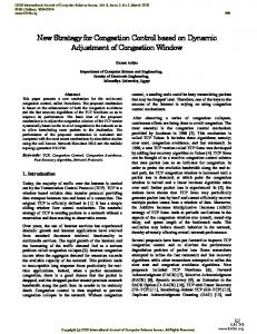
Time Figure 1.

τ could, in this case, be directly adopted and overwrites the minima history (s min). In summary: •

For t ∈ [t0 , t0 + µ]: ◦ If τ > minµ ⇒ minµ = minµ ◦ If τ < minµ ⇒ minµ = τ ◦ If τ < s min ⇒ s min = τ

•

For t = t0 + µ: If minµ > s min ⇒ s min = (1−α)∗s min+α∗minµ

C. How to Reach a Stable Behaviour? The goal of Eclipse is to achieve a stable behaviour without responding to temporary fluctuations. In order to have a base for its calculation, Eclipse holds minimum (minµ ) and maximum (maxµ ) OWD values for the last time interval µ. The current minµ and maxµ are integrated in the smoothed values s min and s max. We denote the way s min and s max are computed as one-way smoothing. This will be further explained in Subsubsection III-C1. The adaptation of the smoothed values occurs at the end of the adaptation interval µ, which is dynamically calculated. It is enlarged when competing traffic is causing periodical variation of the delay (e.g., filling and emptying of router buffers caused by a loss-based flow on the bottleneck) in order to decrease the impact of these interferences. In contradiction to this, µ is decreased when the delay is stable, in order to be able to react to future changes and to adopt them quickly as it will be explained in detail in Subsubsection III-C2). 1) One-Way Smoothed Values: The one-way smoothing of the values is different for minimum and maximum values. For minimum delays, the calculation is performed as follows: smaller OWDs overwrite s min, while higher values are partly added to the history. Let us consider an example where a new OWD τ has been received. Depending on the difference between τ and the current s min, the calculation should be performed in a different way. The case of τ > s min could be understood as a new permanent change in the route, which caused a higher constant delay. But τ does not have a large impact on s min. However, a permanent topology modification means that the next measurements would also be higher and this would make s min converge to the characteristics of the new topology after a certain amount of new OWD measurements. If the higher value τ is an outlier, it would just have a minor impact on the smoothed value and s min would re-converge after a short time to the original value. In contrast to this, the case of τ < s min is different, since a smaller value is definitely a more realistic value, whether it is caused by a topology modification or by buffer deflation.

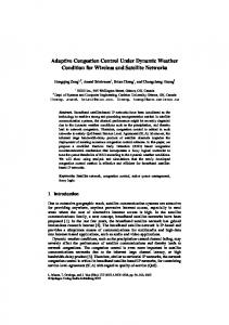
Adaptation Interval µ and Tendency Recognition

α ∈ [0, 1] is a smoothing factor. In this case, higher α values can cause a better smoothing and more steady values. Thus, it would be possible to filter out short-term outliers. On the other hand, lower values make the smoothed value respond faster to permanent changes. For the parameterisation of α and in order to get a good balance between ignoring outliers and reacting to changes, we decided to base on experiences with RTT measurements and adopted the value of α = 1/8, which is typically used for computing the smoothed RTT for TCP [14]. We decided also to only use segments that have been transmitted once, in order to get more accurate values and to avoid the ambiguity created by retransmitted segments [14]. For the calculation of s max, higher values overwrite the smoothed value, while lower values are added to the history: •

For t ∈ [t0 , t0 + µ]: ◦ If τ < maxµ ⇒ maxµ = maxµ ◦ If τ > maxµ ⇒ maxµ = τ ◦ If τ > s max ⇒ s max = τ

•

For t = t0 + µ: If maxµ < s max ⇒ s max = (1 − α) ∗ s max + α ∗ maxµ

2) Dynamic Calculation of the Adaptation Interval µ: Clearly, it is important how long the algorithm should remember old OWDs. LEDBAT bases on a sliding window mechanism (in most of the cases of length 10), where minimum values over one minute intervals are held. As explained in Subsection II-B, this leads to base delay growth, while dealing with long-lived flows or with late reactions to topology changes. For Eclipse, we move away from these static values as well as from the sliding window mechanism and adopt a simpler way, based on a single time interval. Its length µ is calculated on the basis of the network behaviour. The idea behind this is to recognise the delay variation tendency and to hide the variations between the minimum and maximum values, measured within the old interval.

Learning phase

Figure 2.

Tendency Recognition for Reno and Eclipse Flow sharing a Bottleneck

S1

D1 R1

R2

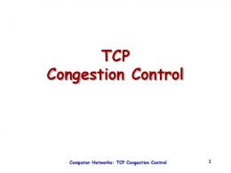
Sn Figure 3.

Tendency recognized

Dn

Simulation Topologies

Let us for instance consider the abstract example shown in Figure 1. It represents the variation of the OWD values measured by Eclipse while sharing a bottleneck with a competing Reno flow. The algorithm holds the minimum value during an interval µ. At the end of µ, minµ is integrated into s min. Choosing a non-convenient interval, such as [t0 , t1 ], would lead to minµ = τa which is higher than the real minimum (here: τb ). In the example shown, the interval [t2 , t3 ], would lead to more suitable minµ = τb and with it filter the variation caused by the competing flow. The same would apply for the maximum delay. The adaptation interval µ is now calculated as follows: µ = t maxµ − t minµ , where t minµ is the time when the minimum delay (minµ ) has been observed. Similarly, t maxµ is the time when the maximum delay (maxµ ) has been measured. The difference between the time when the maximum and the minimum has been registered builds the base for the new interval. Since at the end of the adaptation interval µ the s min and s max values are calculated, the length of this interval has a high impact on the behaviour of the algorithm. Figure 2 provides an example: here, two flows are sharing a bottleneck. First a Reno flow is started, a few seconds later an Eclipse flow is also scheduled. The figure shows the different delays measured and calculated by Eclipse. This experiment shows how far Eclipse is able to recognise the tendency. After a short learning phase, µ is adapted to the network behaviour and s min as well as s max almost stop reacting to undesired delay changes caused by the Reno flow. IV.

S IMULATION S ETUP

For the evaluation, we considered the topologies illustrated in Figure 3. Here, two communication partners (S1 and D1) are transferring data via a shared link. The complete capacity of the core link is denoted as ρcore . The flow between S1

and D1 is denoted as F1 . The bandwidth occupied by F1 is denoted as B1 . For concurrency evaluation experiments, this topology can be extended with n-1 additional flows. For our evaluation, we have utilised the OMN E T++based INET framework. The CC mechanisms considered in this paper have been implemented in the SCTP simulation model [15], [16] with the real-time transport protocol (RTP) [17] model form [18]. Unless otherwise specified, the following parameters have been configured: the core link capacity is ρcore =5 Mbit/s. The access link capacity is ρn =100 Mbit/s. No additional delay has been added on the links. FIFO queues with a maximum size of 100 packets have been configured on the routers. The sender has been saturated (i.e. it has tried to transmit as much data as possible); the message size has been set to 1,452 bytes at an MTU of 1,500 bytes. In the first part of the evaluation, the results are described based on single runs in order to show the basic behaviour over time. For parameter studies, 50 runs are performed in order to ensure a sufficient statistical accuracy. The results plots show the average values and their corresponding 95% confidence intervals. V.

E VALUATION

In the following, we are going to evaluate our new CC by showing to which extent it is able to efficiently utilise the spare capacities with a minimum of self-induced delay and how it deals with LEDBAT-specific issues, such as base delay growth, the latecomer issue and inter-protocol fairness in general. A. Use Only Spare Capacity The first results of the evaluation are presented in Figure 4 and show the benefits of the Eclipse CC. The behaviour of a flow using a background CC is different, depending on the kind of the competing flow considered. In a first step, we have concentrated on the competition with foreground flows. For this purpose, a Reno flow is started first at t=0s. As long as it stays alone on the link, the Reno flow is able to saturate it. After 10 s, a second flow using the Eclipse CC is started. Reno is quickly eclipsing the background flow. The Eclipse flow is still sending a little amount of data (about 7% of the throughput reached by the Reno flow). At t=25s, the Reno flow was stopped, the Eclipse flow is continuing to send alone and reaches almost the same rate as the Reno flow. At t=60s, a third loss-based flow F3 is started. However, unlike the first two

Figure 4.

Competition with Multiple Kinds of Foreground Flows

flows (F1 and F2 ), which have a high-capacity connection to the router R1, the link between S3 and R1 has a lower capacity (ρ3 =1 Mbit/s). Here, the Eclipse flow behaves as expected. Eclipse decreases its sending rate and is able to use the spare capacity without influencing F3 . At t=80s, the Eclipse flow was stopped in order to show how much F2 was disturbing F3 . Here, the throughput reached by F3 remains the same with or without the competing background flow F2 and shows the background characteristics of the Eclipse flow. B. Delay Benefits with Eclipse In the next part of the evaluation, we highlight the delay benefits related to Eclipse. In a first step, we describe its cwnd behaviour, compare it to other CCs, namely Reno and LEDBAT, and explain its influence on the delay characteristics. For this purpose, each one of them has been started separately and was sending without any competition. The cwnd results are shown in Figure 5 for t ∈[0s,60s]. Even if all three CC were able use the link with the same efficiency (i.e. about 600 KiB/s payload throughput), the variation on the cwnd is different. Reno takes packet loss as the only indication for congestion, assuming that the loss occurs due to packets dropped in full router queues. Operation of lossbased CC results in a periodical filling and emptying of router buffers, which in turn leads to an analogous rise and fall of the queuing delays. Contrarily to the loss-based mechanisms, delay-based algorithms like LEDBAT and Eclipse consider an increasing delay as an additional congestion indicator and therefore regulate their sending rate early in response to filling buffers. This results in a lower congestion window without reducing the throughput with respect to the Reno flow. LEDBAT is increasing its cwnd as long as the estimated queuing delay is staying below the target (here: 100 ms, as recommended by [3, Subsection 3.3]). Once the target is reached, the rate will stabilise and the delay gets stabilised. Compared to Reno, the lower delay induced by LEDBAT is already an improvement. However, LEDBAT still adds, from the design point of view, additional delay on the links, which is not always necessary. Eclipse on the other hand is designed to cause as little delay on the links as possible without having throughput penalties. In the second step of this evaluation, the impact of Eclipse on real-time traffic is considered and compared to other CCs. In fact, the compatibility with real-time traffic is an important goal of a background protocol, since real-time audio and video streams have strict delay requirements and specific bandwidth constraints. In this experiment, a constant bit rate RTP flow is

started at (t=0 s), having a frame rate of 25 Hz and frame size of 20000 B (i.e. a payload bit rate of 4 Mbit/s). An additional delay of 70 ms has been set on the bottleneck link. In a first phase of the experiment, the RTP flow does not stress the access link and is delivered at around the base delay of 70 ms. At t=30 s, a second flow is started with a bulk transfer (i.e. a saturated sender). In order to show the impact of the different CCs, the CC of the second flow is varied between Reno, LEDBAT and Eclipse. We observe the end-to-end delay of the RTP messages to see if they remain in an acceptable range for the media flow (see Figure 6(a)). Since the end-to-end delay of the media data is coupled to the delay of the concurrent flows, a delay increase is noticed in all the cases: RTP-Reno, RTP-LEDBAT and RTP-Eclipse. Particularly for the loss-based case (RTP-Reno), the delay is pushed to a very high value that could make the RTP flow unusable. In fact, when a flow using this CC is transmitting along the same path as a real-time transmission, all flows sharing the bottleneck suffer from the same queuing delay curve. This may result in an intolerable delay for interactive media communications [19]. The LEDBAT curve in this case shows another issue related with this CC mechanism: from the design point of view, LEDBAT adopts the Target = 100 ms as a value that is supposed to be suitable for media flows [3], [20]. While being reasonable in fast networks with a low base delay, it lacks of flexibility in other scenarios, e.g. in case of bufferbloat [21]. In this experiment, the RTP end-to-end delay, originally around 70 ms, suffers an increase of about 100 ms after the LEDBAT flow is started and is pushed over the suitable limit. LEDBAT in fact causes the pre-existing delay to rise by 100 ms instead of keeping it at or below that Target. This fact shows that LEDBAT’s choice to implement a constant delay impact is more of a downside in delay-sensitive environments. In contradiction to it, Eclipse considers the complete end-to-end delay instead of only the queuing delay. The target owd Eclipse intends to reach includes both, base and queuing delay, and is a dynamical value that is adapted on the fly to the network conditions. This makes Eclipse reach a marginal self-induced delay and with it minimally influences the RTP flow as shown in Figure 6(a). The benefit related with Eclipse is also highlighted in the next part of the evaluation. The figure shows the Inter-Frame Arrival Time (IFAT), which is the time interval between two successive frames. Since the source Video has a sample rate of 25 Hz, each frame has a playback duration of around 1s 40 ms ( 25 frames/s ) and is sent at this interval to the receiver. If the IFAT is unsteady, the video codec has to compensate

100 50

ψ=Eclipse ψ=LEDBAT ψ=Reno

0

CWND [KiB]

150

Congestion Control ψ

0

Figure 5.

5

10

15

20

25

30 Time t [s]

35

40

45

50

55

60

The Congestion Window of Different CCs while Alone on a Link

150

250

ψ=RTP−Eclipse ψ=RTP−LEDBAT ψ=RTP−Reno

0 50

OWD [ms]

350

Congestion Control ψ

20

25

30

35

40 Time t [s]

45

50

55

60

(a) RTP End-to-End Delay 200

Congestion Control ψ

100 0

50

IFAT [ms]

150

ψ=RTP−Eclipse ψ=RTP−LEDBAT ψ=RTP−Reno

20

25

30

35

40 Time t [s]

45

50

55

60

(b) RTP Inter-Frame Arrival Time (IFAT) Figure 6.

Impact of Different CCs on Real-Time Traffic

this delay by calculating a jitter and effects may range from extra playback delay, which will eventually hurt real-time communication, to dropped frames, which will cause stuttering and image loss. Figure 6(b) shows that for the RTP flow the IFAT is stable at around 40 ms while it is alone on the link (t=0 s to t=30 s). After the second flow is started, beside the very high values during the slow start phase of the Reno flow (up to half a second), a periodical increasing of the IFAT values can be observed, caused by the typical periodical filling and emptying of router buffers that pushes the IFAT to intolerable values. In contradiction to it, the values for both, LEDBAT and Eclipse, are still around the expected value of 40 ms.

To sum up, LEDBAT and Eclipse have an IFAT value at around 40 ms, which makes a playback without stuttering or image loss possible. However, the high delay produced by LEDBAT causes a high playback delay, which could result in a serious disadvantage to real-time communication.

C. The Long-Term Behaviour LEDBAT has difficulties handling flows running for a long period of time, as explained in Subsection II-B. Depending on the base history window length, minimum values are dropped after a certain time span and the algorithm starts using newer values. This makes LEDBAT adapt its base delay and adds additional 100 ms for the end-to-end delay every 10 minutes. In this subsection, we show how Eclipse handles this issue. For this purpose, one LEDBAT and one Eclipse flow have been started consecutively on a single path without competition. To explicitly show the long-term behaviour of both CC algorithms, the transmission time has been set to 2600 s. The results are shown in Figure 7, where we can observe the variation of the end-to-end delay. In this scenario, no additional delay has been configured on the links. LEDBAT assumes that the queue is empty when it starts sending. After a transient phase, it is able to stabilise the

Figure 7.

Base Delay Growth for LEDBAT and the Improvement with Eclipse

delay at the sum of the base delay and the pre-defined Target (here: 100 ms, as recommended by [3, Subsection 3.3]). Since LEDBAT is only able to remember the minimum values that have been measured in the last 10 minutes (60 s × 10 the window length), it forgets the original minimum delay at t=600 s and adopts the previously induced delay as its new base delay. Therefore, the LEDBAT flow increases the induced queuing delay by additional 100 ms. At t=1200s, LEDBAT again measures the minimum of the last interval and tries to add 100 ms to the overall delay. This time it exceeds the maximum rate supported by the buffer. Due to the now occurring packet loss, LEDBAT falls back to the Reno behaviour and halves its cwnd. As this back off does not completely empty the buffer, no accurate base delay measurement can be obtained and LEDBAT again exceeds the maximum router capacity by adding its target delay, which again produces packet loss. Contrarily to LEDBAT, Eclipse bases its calculation on the last view of the network and does not need to hold older values. In addition, the own induced delay is always a small portion from the difference between the minimum and the maximum. This means that the target owd is, under normal circumstances, always below the maximum delay. This makes it unlikely that an Eclipse flow fills up a router buffer completely and forces it to start dropping packets. As can be seen in Figure 7, the Eclipse flow reaches an average OWD of about 9.7 ms over the complete measurement time. D. Fairness between Eclipse Flows and the Latecomer Issue One of the most known issues related to LEDBAT is the latecomer advantage. In this subsection, we therefore analyse the intra-protocol fairness. The way LEDBAT performs the estimation of the base delay heavily depends on the start time of the flow. In fact, while the first flow arriving at an empty bottleneck correctly measures the base delay, a subsequent flow accounts the queuing delay of the first one in its base delay measurement, thus setting a higher target delay. Therefore, the second flow will aggressively take over the target share of the first one, eventually entering a possibly persistent unfair state [9]. The unfairness effect can be easily observed in Subfigure 8(a): here, we have started multiple flows and varied the number of running flows every 30 s. While the first flow (LEDBAT 1) is able to reach a reasonable throughput when being alone on the link, the behaviour becomes unfair after 30 s as soon as LEDBAT 2 is started. After a short period of time, LEDBAT 2 is claiming the biggest part of the bandwidth.

With LEDBAT 3 beginning to send, LEDBAT 2 is pushed over its target and is forced to decrease its sending rate. After a while, the maximum buffer size is reached and packet loss occurs. Here, a smaller base delay is measured. However, it is still including queuing delay and no fair distribution of the bandwidth is reached. In order to deal with this issue, Eclipse has been designed with a focus on the intra-protocol fairness. It is designed to cause an additional delay δ to the minimum delay measured in the past short time period. The calculation of δ is based on the difference between the maximum and minimum delay measured in this time period µ. The value of µ is kept as small as possible, in order to give an opportunity for new-coming flows to converge to the same minimum and maximum seen by older flows. This makes it possible for new flows to get the same view on the network state and to measure the same minimum and maximum values and with it to converge – after a short transient phase – to the same throughput. In order to demonstrate this effect, we repeated the same simulation with the Eclipse CC. The results of this simulation are shown in Subfigure 8(b). Obviously, the first flow (Eclipse 1) is able to use the full capacity. At t=30s, Eclipse 2 is started. After a short transient phase, the capacity is fairly shared between both flows. The same is the case for 3 flows at t ∈[60s,90s]. At t=90s, Eclipse 1 is stopped, and the available capacity is apportioned between Eclipse 2 and Eclipse 3. The same applies for t ∈[120s,150s], where Eclipse 2 – now alone on the link – is able to get all the capacity and at t ∈[150s,190s], where both – Eclipse 2 and Eclipse 4 – each get half of the capacity. E. Behaviour in a Large Aggregation Regime In this last part of the evaluation, the behaviour of both background CCs – LEDBAT and Eclipse – is compared in a large aggregation regime in order to determine to which extent they are able to fulfil the background goals when there are a large number of foreground flows. In this setup, the topology shown in Figure 3 is used again. The total number of flows sharing the bottleneck consisted of nB background flows with nB ∈ {1, 3} and nF foreground flows with nF ∈ [1..10]. All flows are scheduled at different start times that are randomly chosen between t=0.9 s and t=40 s. The simulation run time has been 300 s. The data gathered during the first 60 s is ignored in order to assure that all the flows are already started and the system has converged to a stable state. The results plots show the average values over 50 runs with their corresponding 95% confidence intervals.

600 400 200

ψ=LEDBAT 1 ψ=LEDBAT 2 ψ=LEDBAT 3 ψ=LEDBAT 4

0

Throughput [KiB/s]

Flow ψ

0

20

40

60

80

100 Time t [s]

120

140

160

180

(a) LEDBAT

200

400

600

ψ=Eclipse 1 ψ=Eclipse 2 ψ=Eclipse 3 ψ=Eclipse 4

0

Throughput [KiB/s]

Flow ψ

0

20

40

60

80

100 Time t [s]

120

140

160

180

(b) Eclipse Figure 8.

Throughput of Multiple Simultaneous Eclipse/LEDBAT Flows

The results of the simulation are shown in Figure 9. This simulation confirmed the fairness capabilities of the Reno congestion control, since all Reno flows sharing the bottleneck link were able to reach the same throughput values even for higher nF values. For this reason, the graph was simplified and only a representative curve (the red line) describing the average throughput reached by all Reno flows for different values of nF is shown in both subfigures. In this analysis we decided to consider only the case of 1 and 3 background flows representing for example one host or one host and two smart phones connected to a DSL router. Obviously much more background flows could be started, however it is very unlikely that all users are downloading multiple videos and updates in the same time. The throughput reached by one background flow or the average of all 3 flows is described by the blue lines. Subfigure 9(a) shows severe issues related with LEDBAT. For nB = 1, LEDBAT is able to keep its cwnd in a stage where the queues are still not fully occupied and only experience a small number of losses. Here, only a small room for variation remains for the Reno flows which are pushed to experience too many losses, their windows is penalized and with it the throughput decreased. For the number of foreground flows growing on the bottleneck link, LEDBAT is not only unable to stay in the background, but also shows severe fairness issues by claiming more resources than the foreground flows. With nB = 3, since every later coming LEDBAT flow tries to add new self-induced delay on the link, all LEDBAT flows are pushed out of the comfortable zone, run in a loss case and fall back to standard loss-based TCP-compatible behavior. For lower values of nF , we see that the foreground are still getting the bigger part of the resources but they are are highly influenced by background flows. For higher values of nF ,

all fore and background flows behave TCP-compatible and converge to the same throughput. In contradiction to it, as shown in Subfigure 9(b), Eclipse shows in all combinations a stable behavor. Due to the dynamical adaptation of Eclipse to the network characteristics, it is able to stay around a buffer level where it is unlikely to experience losses. Even for the case of nB = 3, the Eclipse curve shows small confidence intervals, which confirms the intra-protocol fairness of Eclipse. In fact, all Eclipse flows experience similar maximum and minimum values and together with the mechanisms explained in Section III-C, all Eclipse flows are able to converge to the same values. The transparency to foreground flows is here confirmed and beside of minimal throughput values caused by the probing traffic of this protocol, the Eclipse flow is able to stay in the background even for higher values of nF . VI.

C ONCLUSIONS AND F UTURE W ORK

In this paper, we have introduced Eclipse as a new congestion control mechanism for background traffic. We do not claim to have a perfect CC and certainly, there is room for improvement. However, we are convinced that Eclipse could bring a significant benefit for both, the end-users and the network. That is; a “normal” end-user can easily make use of it (e.g. for downloading system updates during a video phone call). We are convinced that this mechanism can provide a significant advantage for services such as cloud-based file synchronisation or system updates. In this work, we have presented a basic evaluation with simulations. We are currently working on a more practical evaluation, especially with measurements in real-world Internet setups. Therefore, we are also going to analyse them in reality in the N OR N ET testbed [22]–[24], a large-scale distributed

Average Throughput per Flow [Mbit/s] 1 2 3 4 5

Congestion Control ψ / Number of Background Flows nB 1: ψ=LEDBAT, nB=1 2: ψ=LEDBAT, nB=3 3: ψ=Reno, nB=1 4: ψ=Reno, nB=3

[7]

[8]

[9]

[10]

0

[11] 1

2

3

4

5

6

7

8

9

10

Number of Foreground Flows nF

[12]

(a) LEDBAT

Average Throughput per Flow [Mbit/s] 1 2 3 4 5

Congestion Control ψ / Number of Background Flows nB 1: ψ=Eclipse, nB=1 2: ψ=Eclipse, nB=3 3: ψ=Reno, nB=1 4: ψ=Reno, nB=3

[13]

[14]

[15]

0

[16]

1

2

3

4

5

6

7

8

9

10

Number of Foreground Flows nF

(b) Eclipse Figure 9. Throughput of an Eclipse/LEDBAT Flow in the Existence of multiple Simultaneous Foreground Flows

[17]

[18]

[19]

research platform in the Internet. Such a practical analysis is finally also necessary in order to contribute our research results into the IETF, in order to transfer our research to application. Particularly, for our testbed analysis, we will also examine multi-path transport aspects [25]. R EFERENCES [1]

[2]

[3] [4] [5]

[6]

A. Venkataramani, R. Kokku, and M. Dahlin, “TCP Nice: A Mechanism for Background Transfers,” ACM SIGOPS Operating Systems Review, vol. 36, pp. 329–343, Dec. 2002. A. Kuzmanovi´c and E. W. Knightly, “TCP-LP: Low-Priority Service via End-Point Congestion Control,” IEEE/ACM Transactions on Networking, vol. 14, no. 4, pp. 739–752, Aug. 2006. S. Shalunov, G. Hazel, J. R. Iyengar, and M. K¨uhlewind, “Low Extra Delay Background Transport (LEDBAT),” IETF, RFC 6817, Dec. 2012. M. Welzl and D. Ros, “A Survey of Lower-than-Best-Effort Transport Protocols,” IETF, Informational RFC 6297, Jun. 2011. L. S. Brakmo, S. W. O’Malley, and L. L. Peterson, “TCP Vegas: New Techniques for Congestion Detection and Avoidance,” in Proceedings of the ACM SIGCOMM Conference, London/United Kingdom, Aug. 1994, pp. 24–35. C. Jin, D. X. Wei, and S. H. Low, “FAST TCP: Motivation, Architecture, Algorithms, and Performance,” in Proceedings of the 23rd IEEE INFOCOM, St. Maarten/Netherlands Antilles, Mar. 2004, pp. 2490– 2501.

[20]

[21]

[22]

[23]

[24]

[25]

Y.-C. Chan, C.-L. Lin, C.-T. Chan, and C.-Y. Ho, “CODE TCP: A Competitive Delay-Based TCP,” Computer Communications, vol. 33, no. 9, pp. 1013–1029, Jun. 2010. G. Carofiglio, L. Muscariello, D. Rossi, and C. Testa, “A HandsOn Assessment of Transport Protocols with Lower Than Best Effort Priority,” in Proceedings of 35th Annual IEEE Conference on Local Computer Networks (LCN), Denver, Colorado/U.S.A., Oct. 2010, pp. 8–15. G. Carofiglio, L. Muscariello, D. Rossi, and S. Valenti, “The Quest for LEDBAT Fairness,” in Proceedings of the IEEE Global Communications Conference (GLOBECOM), Miami, Florida/USA, Dec. 2010, pp. 1–6. D. Ros and M. Welzl, “Assessing LEDBAT’s Delay Impact,” IEEE Communications Letters, vol. 17, no. 5, pp. 1044–1047, May 2013. ¨ u Alay, “Multi-Path Transport over S. Ferlin, T. Dreibholz, and Ozg¨ Heterogeneous Wireless Networks: Does it really pay off?” in Proceedings of the IEEE Global Communications Conference (GLOBECOM), Austin, Texas/U.S.A., Dec. 2014, pp. 5005–5011. ——, “Tackling the Challenge of Bufferbloat in Multi-Path Transport over Heterogeneous Wireless Networks,” in Proceedings of the IEEE/ACM International Symposium on Quality of Service (IWQoS), Hong Kong/People’s Republic of China, May 2014, pp. 123–128. ¨ u Alay, and A. Kvalbein, “Measuring the S. Ferlin, T. Dreibholz, Ozg¨ QoS Characteristics of Operational 3G Mobile Broadband Networks,” in Proceedings of the 4th International Workshop on Protocols and Applications with Multi-Homing Support (PAMS), Victoria, British Columbia/Canada, May 2014, pp. 753–758. P. Karn and C. Partridge, “Improving Round-Trip Time Estimates in Reliable Transport Protocols,” ACM Transactions on Computer Systems (TOCS), vol. 9, pp. 364–373, Nov. 1991. I. R¨ungeler, M. T¨uxen, and E. P. Rathgeb, “Integration of SCTP in the OMNeT++ Simulation Environment,” in Proceedings of the 1st ACM/ICST International Workshop on OMNeT++, Marseille, Bouchesdu-Rhˆone/France, Mar. 2008. T. Dreibholz, M. Becke, H. Adhari, and E. P. Rathgeb, “On the Impact of Congestion Control for Concurrent Multipath Transfer on the Transport Layer,” in Proceedings of the 11th IEEE International Conference on Telecommunications (ConTEL), Graz, Steiermark/Austria, Jun. 2011, pp. 397–404. H. Schulzrinne, S. L. Casner, R. Frederick, and V. Jacobson, “RTP: A Transport Protocol for Real-Time Applications,” IETF, Standards Track RFC 3550, Jul. 2003. M. Becke, E. P. Rathgeb, S. Werner, I. R¨ungeler, M. T¨uxen, and R. R. Stewart, “Data Channel Considerations for RTCWeb,” IEEE Communications Magazine, vol. 51, no. 4, pp. 34–41, Apr. 2013. T. Szigeti and C. Hattingh, End-to-End QoS Network Design: Quality of Service in LANs, WANs, and VPNs Quality of Service Design Overview. Cisco Press, Nov. 2004. Telecommunication Standardization Sector of the ITU, ITU-T Recommendation G.114: Transmission Systems and Media : General Recommendations on the Transmission Quality for an Entire International Telephone Connection : One-Way Transmission Time. International Telecommunication Union, 2003. V. Cerf, V. Jacobson, N. Weaver, and J. Gettys, “BufferBloat: What’s Wrong with the Internet?” ACM Queue, vol. 9, no. 12, pp. 10–20, Dec. 2011. T. Dreibholz, “NorNet at NICTA – An Open, Large-Scale Testbed for Multi-Homed Systems,” Invited Talk at National Information Communications Technology Australia (NICTA), Sydney, New South Wales/Australia, Jan. 2015. E. G. Gran, T. Dreibholz, and A. Kvalbein, “NorNet Core – A MultiHomed Research Testbed,” Computer Networks, Special Issue on Future Internet Testbeds, vol. 61, pp. 75–87, Mar. 2014. T. Dreibholz and E. G. Gran, “Design and Implementation of the NorNet Core Research Testbed for Multi-Homed Systems,” in Proceedings of the 3nd International Workshop on Protocols and Applications with Multi-Homing Support (PAMS), Barcelona, Catalonia/Spain, Mar. 2013, pp. 1094–1100. T. Dreibholz, X. Zhou, and F. Fa, “Multi-Path TCP in Real-World Setups – An Evaluation in the NorNet Core Testbed,” in 5th International Workshop on Protocols and Applications with Multi-Homing Support (PAMS), Gwangju/South Korea, Mar. 2015, pp. 617–622.