Climate simulations for past, present, and future have enabled macroecologists and biogeographers to combine data on species' occurrences with detailed ...
Biodiversity Informatics, 10, 2015, pp. 1-‐21
ECOCLIMATE: A DATABASE OF CLIMATE DATA FROM MULTIPLE MODELS FOR PAST, PRESENT, AND FUTURE FOR MACROECOLOGISTS AND BIOGEOGRAPHERS MATHEUS S. LIMA-RIBEIRO1, SARA VARELA2,3, JAVIER GONZÁLEZ-HERNÁNDEZ4, GUILHERME DE OLIVEIRA5, JOSÉ ALEXANDRE F. DINIZ-FILHO6, LEVI CARINA TERRIBILE1 1 Laboratório de Macroecologia, Universidade Federal de Goiás, Regional Jataí, Cx. Postal 03, 75804-020, Jataí, GO, Brazil 2 Departamento de Ciencias de la Vida, Edificio de Ciencias, Campus Externo, Universidad de Alcalá, 28805 Alcalá de Henares, Madrid, Spain 3 Museum für Naturkunde. Leibniz Institute for Evolution and Biodiversity Science. Invalidenstr. 43, 10115 Berlin, Germany 4 Carmelitas Descalzos, 5. 45002, Toledo, Spain 5 Laboratório de Biogeografia da Conservação e Comportamento Animal, Universidade Federal do Recôncavo da Bahia (UFRB), Centro de Ciências Agrárias, Ambientais e Biológicas (CCAAB), Setor de Biologia, Rua Rui Barbosa 710, Centro 44380-000, Cruz das Almas, BA, Brazil 6 Departamento de Ecologia, ICB, Universidade Federal de Goiás, Cx. Postal 131, 74001-970, Goiânia, GO, Brazil Abstract.—Studies in biogeography and macroecology have been increasing massively since climate and biodiversity databases became easily accessible. Climate simulations for past, present, and future have enabled macroecologists and biogeographers to combine data on species’ occurrences with detailed information on climatic conditions through time to predict biological responses across large spatial and temporal scales. Here we present and describe ecoClimate, a free and open data repository developed to serve useful climate data to macroecologists and biogeographers. ecoClimate arose from the need for climate layers with which to build ecological niche models and test macroecological and biogeographic hypotheses in the past, present, and future. ecoClimate offers a suite of processed, multi-temporal climate data sets from the most recent multi-model ensembles developed by the Coupled Modeling Intercomparison Projects (CMIP5) and Paleoclimate Modeling Intercomparison Projects (PMIP3) across past, present, and future time frames, at global extents and 0.5° spatial resolution, in convenient formats for analysis and manipulation. A priority of ecoClimate is consistency across these diverse data, but retaining information on uncertainties among model predictions. The ecoClimate research group intends to maintain the web repository updated continuously as new model outputs become available, as well as software that makes our workflows broadly accessible. Key words.—climate data, raster, bioclimatic variables, general circulation models, kriging, downscaling, Pleistocene, Pliocene, Holocene.
The availability of spatially explicit data layers summarizing past, present, and future climate conditions has stimulated the fields of biogeography and macroecology greatly in the last two decades. For instance, the pioneering WorldClim repository1 (Hijmans et al., 2005) enabled researchers to integrate data on species’ geographic occurrences with detailed information on climate conditions through time to predict biological responses across large spatial and temporal scales. In tandem with the climate data, access to vast data
1
http://www.worldclim.org.
resources about biodiversity (e.g., GBIF2, Paleobiology Database3, speciesLink4), and exciting new computational tools (e.g., the new R packages; rgbif: Chamberlain et al., 2013; rAvis: Varela et al., 2014a; paleobioDB: Varela et al., 2014b), have facilitated fundamental analyses by macroecologists and biogeographers on broad scales. The multi-temporal climate data have been used to explore effects of past (Varela et al., 2015a) and future (Thomas et al., 2004)
2
http://www.gbif.org. http://www.paleobiodb.org. 4 http://splink.cria.org.br. 3
1
Biodiversity Informatics, 10, 2015, pp. 1-‐12
climate change; to understand past extinction events (Lima-Ribeiro et al., 2013a); and to test hypotheses concerning population dynamics (Barrientos et al., 2014), evolutionary processes (Araújo et al., 2013; Saupe et al., 2014), and ecological dynamics (Martínez-Meyer et al., 2004; Martínez-Meyer and Peterson, 2006). Data layers summarizing climatic information are created by interpolating continuous surfaces from real (generally point-based) observations, or by modeling conditions based on complex simulations describing key processes of atmospheric and ocean circulation, the so-called general circulation models (GCMs; Braconnot et al., 2007). For instance, New et al. (2002), Hijmans et al. (2005), and Kriticos et al. (2012) provide interpolated data layers for modern climates based on observations from almost 50,000 weather stations worldwide; ~100 fossil pollen records from the Last Glacial Maximum (LGM - 21 ka, Bartlein et al., 2011; Harrison et al., 2014) and midPliocene (Dowsett et al., 2012) made possible building layers for past continental climates. However, a dearth of detailed fossil data linking time and space has hindered building reliable data layers from paleobiological observations. Obviously, future climatic conditions are not accessible via observation. Consequently, climatologists have invested in GCMs to simulate global climate over long time periods, and connect climates of the deep geological past through the present to future conditions. Climatologists tune GCMs based on boundary conditions such as orbital parameters, solar forcing, greenhouse gas concentrations, CO2 emissions, land-use, and ice coverage, coupled with atmospheric, vegetation, and ocean dynamics (Braconnot et al., 2007). Via these intensive computer simulations, climatologists have predicted global climates for past (Miocene, Pliocene, late Quaternary), present (pre- and postindustrial), and future conditions (end of 21st century; Taylor et al., 2012). Still, climate model outputs are not at all user-friendly for most macroecologists and biogeographers. Outputs are normally formatted as complex text files (e.g., netCDF format), which are not trivial to process; even to understand the acronyms used for identifying the dozens of climatic variables and model parameters can be challenging.
Macroecologists and biogeographers are used to working with data layers in the form of raster images or simple ASCII text files. Spatial resolution also differs among GCMs, precluding direct incorporation into spatial analyses without complex downscaling procedures. Given, then, the often complex and inaccessible nature of GCM outputs, and yet the great interest in multi-temporal climate data and their enormous applicability to important questions in macroecology and biogeography, we decided to process climate layers from multiple GCMs, and make them available on a free and open web repository: ecoClimate5. ecoClimate offers a wide suite of climate data layers from the most recent multi-model ensembles published as part of the Coupled Model Inter-comparison Project (CMIP5; Taylor et al., 2012) and the Paleoclimate Modeling Intercomparison Project (PMIP3) across past, present and future time frames, at global extents and 0.5° spatial resolution. Data are provided in formats easily incorporated in analyses via common platforms and popular GIS software. METHODS Raw climatic variables We accessed climatic simulations from most recent generations of coupled atmosphere-ocean general circulation models (AOGCMs) available in the CMIP5 and PMIP3 databases (Table 1). The AOGCMs comprised multi-model ensembles for longterm experiments: past ("PlioExp2a", "lgm", and "midHolocene" experiments), present ("piControl" and "historical" experiments) and future scenarios ("RCPs" experiments for different CO2 emission scenarios), although some specific outputs are not yet available from some modeling groups (Table 2). AOGCMs run long-term simulations for preindustrial scenario (~1760), a control experiment (piControl) for stabilizing climate predictions and model evaluation, and then simulate climates for different time slices, according to specific boundary conditions. Besides pre-industrial, current conditions are also simulated for historical periods, providing climatic conditions for the 20th century (indeed, the industrial period from 1850 to 2005). Future conditions are
5
http://www.ecoclimate.org/.
2
3
13
12
http://cmip-pcmdi.llnl.gov/cmip5/. http://pmip3.lsce.ipsl.fr/.
MPI-ESM-P MRI-CGCM3
MIROC-ESM
IPSL-CM5ALR
Atmosphere and Ocean Research Institute (University of Tokyo), National Institute for Environmental Studies, and Japan Agency for Marine-Earth Science and Technology, Japan Max Planck Institute for Meteorology, Germany Meteorological Research Institute, Japan
Institut Pierre Simon Laplace, France
FGOALS-g2
NASA Goddard Institute for Space Studies, USA
Freie Universität Berlin, Germany
Modeling Center National Center for Atmospheric Research, USA Centre National de Recherches Meteorologiques / Centre Europeen de Recherche et Formation Avancees en Calcul Scientifique, France
National Key Laboratory of Numerical Modeling for Atmospheric Sciences and Geophysical Fluid Dynamics (LASG) / Institute of Atmospheric Physics (IAP), China
GISS-E2-R
COSMOSASO (FUB)
CNRM-CM5
Model ID CCSM4
2.8° × 2.8° 1.9° x 1.9° 1.1° x 1.1°
3.75° x 1.9°
2.8° × 2.8°
2.5° x 2.0°
3.75° x 3.7°
1.4° x 1.4°
Resolution 0.9° × 1.25°
100 100 100
200
100
100
600
200
Number of years 100
CMIP5/PMIP3 CMIP5/PMIP3 CMIP5/PMIP3
CMIP5/PMIP3
CMIP5/PMIP3
CMIP5/PMIP3
PMIP3
CMIP5/PMIP3
Source CMIP5/PMIP3
2012 2011 2012
2012
2013
2012
2012
2012
Release 2012
Table 1. Details of the coupled Atmosphere-Ocean General Circulation Models (AOGCMs) available in the ecoClimate database. All simulations were obtained from the r1i1p1 ensemble, except GISS (r1i1p151). The native AOGCM-specific resolutions, in decimal degrees (longitude and latitude), are coarse (1-4º). Most models were run over time series of 100 yr after initial calibration periods. Source: CMIP5, the fifth phase of Coupled Model Intercomparison Project12 and PMIP3, the third phase of Paleoclimate Modeling Intercomparison Project13.
Table 2. ecoClimate layers processed as regards availability of outputs (! indicates available, ✗ indicates not available) from the CMIP5 and PMIP3 working groups. Experiment acronyms: Plio: mid-Pliocene Warm Period (mPWP, ~3.3 to 3.0 million years ago); LGM: Last Glacial Maximum (21,000 years ago); HOL: mid-Holocene (6000 years ago); piControl: pre-Industrial (~1760); Historical (1900-1949); Modern (1950-1999); RCPs: representative carbon pathways, with emission scenarios for the end of the 21st century (2080-2100). Past
AOGCM
CCSM CNRM COSMOS FGOALS GISS IPSL MIROC MPI MRI
Present
Future
Plio
LGM
HOL
piCon.
Histor.
Modern
RCP2.6
RCP4.5
RCP6.0
RCP8.5
! ✗ ✗ ✗ ✗ ✗ ✗ ✗ ✗
! ! ! ! ! ! ! ! !
! ! ✗ ! ✗ ! ! ! !
! ! ! ! ! ! ! ! !
! ! ✗ ! ! ! ! ! !
! ! ✗ ! ! ! ! ! !
! ✗ ✗ ! ! ! ! ✗ !
! ! ✗ ✗ ! ! ! ✗ !
! ✗ ✗ ✗ ! ! ! ✗ !
! ! ✗ ! ! ! ! ✗ !
Table 3. Spatial correlation (Pearson's coefficient, r) among downscaled temperature (above diagonal) and precipitation (below diagonal) layers from distinct techniques. Krige: ordinary kriging; IDW: inverse distance weighting; Splines: thin-plate spline; Trend: trend surface with 12th-order polynomial regression. Krige IDW Splines Trend Natural neighbor
Krige 0.98 0.99 0.84
IDW 0.99 0.97 0.90
Splines 0.99 0.99 0.83
Trend 0.99 0.99 0.99 -
Natural neighbor 0.99 0.99 1.00 0.99
0.99
0.97
0.99
0.83
-
Figure 1. Mean square errors (MSE) among downscaling techniques for (A) temperature and (B) precipitation layers. Note that lowest MSEs come from ordinary kriging method. Krige: ordinary kriging; IDW: inverse distance weighting; Splines: thin-plate spline; Trend: trend surface with 12th-order polynomial regression. 4
Biodiversity Informatics, 10, 2015, pp. 1-‐12
simulated in sequence, out to 2100, following different representative concentration pathways (RCPs) across 21st century (RCP2.6, RCP4.5, RCP6.0, and RCP8.5 experiments). Finally, experiments for past scenarios cover the LGM (Bartlein et al., 2011) and midHolocene (6 ka), key periods representing glacial and interglacial phases related to the last ice age, as well as the mid-Pliocene warm period (mPWP, ~3.3-3.0 Ma). From such AOGCMs (Table 2), we downloaded 4 simulated monthly atmospheric variables: precipitation flux (pr), mean surface temperature (tas), maximum surface temperature (tasmax), and minimum surface temperature (tasmin). All outputs match ensemble member "r1i1p1" (except GISS, which was r1i1p151), assuring compatible outputs among AOGCMs. Because AOGCMs run long-term simulations, we averaged simulated monthly values from the entire native time-series for pre-industrial and past experiments (Table 1) to guarantee reliable long-term means. For the historical experiments, we averaged climate predictions for 1900-1949 (hereafter the “historical” period) and 1950-1999 (hereafter the “modern” period). Future predictions were averaged between 2080 and 2100, thus representing conditions for the end of the 21st century. Temperature variables were transformed from Kelvin to Celsius, and precipitation flux (in mm m-2 s-1) was converted to total monthly precipitation (mm month-1), taking into account a month with 30 days according the specific calendar of 360 days year-1. The original netCDF files with raw AOGCM outputs were processed using the ncdf package in R (Pierce, 2014). Scripts are available openly6. Statistical downscaling: regridding AOGCMspecific native outputs The long-term means for temperature and precipitation variables were downscaled to 0.5° resolution. Our downscaling was actually a regridding procedure instead of a standard interpolation (implications discussed below). Standard interpolations are commonly used for observed climatology to increase resolution, but mainly to create spatially continuous values across a regular grid of
6
https://github.com/ecoclimate.
cells (see details in Harris et al., 2014). Because weather stations are not regularly spatially, this continuity is crucial (see examples in New et al., 2002; and Hijmans et al., 2005). In our case, AOGCMs outputs are already originally gridded and continuous, albeit at coarse resolutions (Table 1), so we regridded raw variables from model-specific native resolutions to a global 0.5° grid. We thus produced climatic layers at a resolution relevant to the spatial scales at which macroecologists and biogeographers are interested, and on a comparable grid system among all AOGCMs. Change-factor approach We followed the change-factor approach to downscaling (Wilby et al., 2004). This approach comprises three steps: (i) compute the change-factor (also called climate change trends or anomalies) between past/future and baseline climate for each raw variable at model-specific native spatial resolution, (ii) downscale change-factor (“smoothing”) and the corresponding baseline climate from each AOGCM to the standard 0.5° resolution, and (iii) apply downscaled change-factor to the downscaled baseline climate to reconstitute values and obtain downscaled layers for past and future climates. In the change-factor approach, current climate layers from weather station interpolations are often used to represent baseline climates from which change-factors are computed (Hijmans and Graham, 2006; Kriticos et al., 2012). We considered three scenarios from AOGCMs as baseline climates (pre-industrial, historical, and modern), taking into account macroecological and biogeographic interests, as has been used in applications such as ecological niche modeling (Terribile et al., 2012; Collevatti et al., 2013a; 2013b; Lima et al., 2014); they also cover time periods for ample biodiversity data exist, and so are potentially useful for models relating organisms to environments. In the first step, change-factors for temperature variables (T change-factors) were computed as the simple difference between past/future and baseline conditions (a standard anomaly in climatology) for each grid cell, for a given AOGCM. For precipitation, changefactors (P change-factors) were computed as ratios of anomalies to corresponding baseline conditions. Ratios are more robust in
5
Figure 2. Maps illustrating the 19 bioclimatic variables available in ecoClimate; red and blue titles indicate maps for temperature and precipitation variables, respectively. For simplicity, maps were built only for the LGM in South America, as predicted by AOGCM CCSM4. However, ecoClimate offers climate data at global extents for multiple periods (Figure 3) and 9 AOGCMs (Table 2), including raw monthly variables. The name and unit of bioclimatic variables are provided in Table 4.
6
Figure 3. Time series illustrating the global extent and multi-temporal characteristic of climate data available in ecoClimate. For illustration, maps show only annual mean temperature (Bio1) across past, present and future time periods from AOGCM CCSM4. However, ecoClimate offers similar time series for 9 AOGCMs (Table 2) and 19 bioclimatic variables (Table 4 and Figure 2). The period "Present" represents the baseline used to downscale time series (pre-Industrial ~1760, Historical 19001949, or Modern 1950-1999; not shown here, but see details in Figure 5). Color scale is standardized across all maps; white, red and blue tones indicate near zero, positive and negative temperatures, respectively. 7
Biodiversity Informatics, 10, 2015, pp. 1-‐12
maintaining original patterns in downscaling when managing large values, as in precipitation (Wilby et al., 2004). In the second step, we used ordinary kriging to downscale both raw T and P change-factors and their respective baseline climates statistically to the standard global 0.5° grid (see details below on kriging methods). In the third step, we applied the downscaled T and P change-factors to the corresponding downscaled baseline layers to obtain downscaled past and future scenarios. This step follows the inverse of the computation in the first step. For temperature, this involves adding the T change-factors to the correspondent baseline temperature value in each grid cell; for precipitation, the values are multiplied by baseline values to unpack ratios on the original precipitation scale. Ordinary kriging method We automated downscaling by coupling functions from the gstat package (Pebesma, 2004) in a script in R (R Development Core Team, 2014). Downscaling was performed using the “krige” kriging function, based on the 12 nearest observations to a given focal point (rather than fitting an inverse distance weighted power from the global neighborhood) and a variogram model. To model the spatial structure in data, we fit a variogram using the “fit.variogram” function, which fits ranges and sills from a variogram model (here a spherical variogram) to a sample variogram. The spherical variogram model was used because it shows a progressive decrease of spatial autocorrelation out to some distance, beyond which autocorrelation is zero, a common spatial structure in climate data (in an exponential model, for example, autocorrelation would disappear completely only at an infinite distance). The sample variogram was obtained using the “variogram” function, following the direction with the largest range (i.e., the omnidirectional model type) in each variable, and assuming a constant trend for variables (i.e., we did not specify predictors to fit sample variograms). Integrating these functions from gstat package in R (Pebesma, 2004) made automating the interpolation procedure possible. Scripts are available
openly at the Internet link given in the footnote7. Sensitivity analyses: comparing downscaling methods Diverse statistical methods have been used for downscaling data and generate standardized, finer-resolution climate surfaces. We used ordinary kriging because it is known to produce reliable regridded surfaces by considering spatial structure in raw gridded variables to minimize variance of errors (Hartkamp et al., 1999). Considering spatial structure in data is an important advantage relative to other simple linear interpolation techniques (e.g., regression methods, see Hartkamp et al., 1999, for an overview); ordinary kriging is desirable here for regridding climatic simulations that reflect the spatial structure of original gridded boundary conditions (e.g., ice sheet, topography, vegetation, insolation). Moreover, because our dataset was based on gridded climatic simulations, it makes no conceptual sense to account for effects on observed climate patterns (e.g., coastal influence, terrain barriers, temperature inversions, which are explicitly accounted by the PRISM method, for example; see Daly et al., 2002), nor linking weather stations along isoclines from irregularly spaced data points (which, for example, would be obtained by thin-plate spline-fitting techniques like ANUSPLIN; see details in Hutchinson and Xu, 2013; see applications in New et al., 2002; Hijmans et al., 2005). However, to avoid doubt about our choices, we spatially downscaled raw temperature mean (tas) and precipitation (pr) variables from AOGCM CCSM4, preindustrial experiment, using other 4 common methods: thin-plate splines, inverse distance weighting, trend surface (best results achieved with 12th-order polynomial regression), and natural neighbor. To compare methods, we correlated all downscaled layers each other, and found them highly spatially concordant with corresponding originally interpolated layers by ordinary kriging (all r > 0.96 for precipitation, except for trend surface method; all r > 0.98 for temperature; Table 3). Moreover, we evaluated the efficiency of each downscaling method by comparing
7
https://github.com/ecoclimate.
8
Table 4. Description of the 19 bioclimatic variables and contribution of raw monthly temperature and precipitation variables used in their calculations, all available in ecoClimate. Tasmin: minimum surface temperature; Tasmax: maximum surface temperature; Tas: mean surface temperature; Pr: precipitation flux. Bioclimatic variables Variable Bio1 Bio2 Bio3 Bio4 Bio5 Bio6 Bio7
Raw variables Tasmin (°C)
Description (name/unit) Annual mean temperature (°C) Mean diurnal range (°C) (mean of monthly (max temp - min temp)) Isothermality (%) (100*Bio2/Bio7) Temperature seasonality (%) (standard deviation *100) Max temperature of warmest month (°C) Min temperature of coldest month (°C) Temperature annual range (°C) (Bio5-Bio6)
Bio8
Mean temperature of wettest quarter (°C)
Bio9
Mean temperature of driest quarter (°C)
Bio10
Mean temperature of warmest quarter (°C)
Bio11
Mean temperature of coldest quarter (°C)
Bio12
Annual precipitation (mm/m2)
Tas (°C)
Precipitation of wettest month (mm/m )
Bio14
Precipitation of driest month (mm/m2) Precipitation seasonality - % (coefficient of variation)
Bio16
Precipitation of wettest quarter (mm/m2)
Bio17
Precipitation of driest quarter (mm/m2)
Bio18
Precipitation of warmest quarter (mm/m2)
Bio19
Precipitation of coldest quarter (mm/m2)
Pr (mm m-2)
! !
!
!
! ! !
! !
! ! ! ! !
! !
! ! !
2
Bio13
Bio15
Tasmax (°C)
!
! !
! ! ! !
9
Biodiversity Informatics, 10, 2015, pp. 1-‐12
values of 5000 random points (n, ~10% of original CCSM4 grid cells) from downscaled (X) and native gridded (Z) layers using mean square errors, as MSE = 1/n*Σ(Xi – Zi)2. From MSE, lower errors indicate more precise methods: downscaled estimates are more similar to corresponding original values. This procedure was repeated 1000 times. Multiple regridded values (finer resolution) matching every AOGCM-native grid cell (coarser resolution) were averaged to allow direct comparison. Kriging showed lowest MSEs for both temperature and precipitation variables (Figure 1). Our sensitivity analyses showed that, although all methods produced downscaled climatic layers with similar spatial patterns (high correlations), ordinary kriging was the most precise for downscaling both temperature and precipitation variables (lowest MSE). Because the climate science community has not established best practices by which to develop higher-resolution climate layers (Hall, 2014), our sensitivity analyses at least guarantee that ordinary kriging represents a good practical choice. Building bioclimatic layers We used the downscaled layers of the 4 raw variables (precipitation, mean temperature, maximum temperature, minimum temperature) for the 12 months of the year to calculate the 19 core bioclimatic variables (Table 4). We followed the standard equations used by WorldClim8, except that BIO1 (annual mean temperature) was obtained directly from AOGCM simulations (variable tas), instead of as an average maximum and minimum temperatures, as implemented in the "biovars" function in the dismo package in R (Hijmans et al., 2013). THE ECOCLIMATE DATABASE The web-repository We created a web-repository, ecoClimate9, to share downscaled bioclimatic layers (Figure 2), as well as the long-term means for raw monthly temperature and precipitation variables. Bioclimatic variables are commonly used in macroecological and biogeographic analyses, like ecological niche modeling. Monthly variables are needed to compute
8 9
http://www.worldclim.org/bioclim. http:///www.ecoclimate.org.
other desirable climate predictors, such as actual and potential evapotranspiration (AET/PET, see AET calculator10). The dataset includes standard 0.5° gridded climate layers for mid-Pliocene (~3.3 to 3.0 Ma), LGM (21 ka), mid-Holocene (6 ka), pre-industrial (~1760), historical (1900-1949), modern (1950-1999) and future conditions (20802100, end of the 21st century), all from updated AOGCMs available in the most recent CMIP5 and PMIP3 climate modeling projects (Figure 3). Future simulations include four representative concentration pathways (RCPs): RCP2.6 (low emissions scenario), RCP4.5 and RCP6.0 (intermediate emissions scenarios), and RCP8.5 (high emissions scenario; see details about climate scenarios in Taylor et al., 2012). A distinctive attribute of ecoClimate is its multi-model and multi-temporal coverage (Figure 4). This distinction makes ecoClimate potentially applicable to a multitude of questions commonly asked in macroecology and biogeography. However, in analyses using multi-temporal climatic scenarios, downscaled layers should be matched. For example, past and future layers are genuinely comparable only if downscaled from the same baseline condition (pre-industrial, historical or modern climate; Figure 5). This detail is needed to ensure that climate layers are comparable, and not reflecting differences among baselines. By presenting and serving uniform data from different climatic simulations that are compatible through time, ecoClimate allows users to consider and evaluate apparent differences among AOGCMs (see details on climate modeling uncertainties in Taylor et al., 2012, and Harris et al., 2014). The multiple current climate data available in ecoClimate that were used across the downscaling procedure as baseline scenarios are specific to each AOGCM, instead of a unique standard observed climate (e.g., from interpolations among weather stations), favors keeping modeling uncertainties intact. Therefore, considering the spread of results as available in ecoClimate is crucial to perspectives on the range of potential signals of interest in macroecological and biogeographic studies (see discussion in Varela et al., 2015b).
10
http://geog.uoregon.edu/envchange/software.html.
10
11
Figure 4. Overview of the ecoClimate database, data availability, attributes, and perspectives. ecoClimate offers compatible 0.5° regridded climate layers from the most recent phase of the modeling projects CMIP5 and PMIP3, encompassing multiple AOGCMs and experiments across the past, present, and future. The perspective for keeping ecoClimate complete and up-to-date will require incorporation of further AOGCMs from next-generation experiments; see Meehl et al. 2014. Experiment acronyms: Plio: mid-Pliocene Warm Period (mPWP, ~3.3 to 3.0 million years ago); LGM: Last Glacial Maximum (21,000 years ago); mH: mid-Holocene (6000 years ago); piControl: pre-Industrial (~1760), HIST: historical (originally 1850-2005, but in ecoClimate averaged in Historical 1900-1949 and Modern 1950-1999); RCPs: representative carbon pathways with emission scenarios for the end of the 21st century (2080-2100); LIG: Last InterGlacial (~125,000 years ago); Mio: mid-Miocene Climatic Optimum (mMCO, 17 to 14.5 million years ago). See detail about AOGCMs in Table 1.
Figure 5. Schematic representation of the compatibility pattern among downscaled layers from ecoClimate database. For each AOGCM, three groups of downscaled layers have been derived based on distinct baseline scenarios (pre-Industrial, Historical, Modern). Past and future climate layers are necessarily compatible for a same baseline, but incompatible among baselines. See experiment acronyms in Figure 4.
12
Biodiversity Informatics, 10, 2015, pp. 1-‐12
Using a scenario based on observed climate (see example in Hijmans and Graham, 2006) would reduce variability among AOGCM outputs by relating downscaled past and future layers to the same unique baseline, and could hide potential macroecological and biogeographic responses or underestimate their variation or uncertainty. Not considering the full diversity of potential responses to climate change may compromise many research questions, or even lead to invalid results in many cases (e.g., see the importance of using intact climate uncertainty for phylogeographic inference as discussed in Collevatti et al., 2013b; 2015). Potentiality, applicability, and relevance The data served via ecoClimate are potentially applicable to a multitude of research interests, including numerous questions in macroecology and biogeography, but also in diverse environmental, agricultural and paleobiological sciences (Figure 6). Ecological niche modeling (ENM) and its numerous research purposes, for instance, offer an excellent example. Ecological niche models estimate associations between environmental aspects (most often climate) and known occurrences of species to characterize the range of conditions under which the species’ populations are viable. This suite of methods and ideas has been applied to diverse research purposes: guiding discovery of populations of known (Bourg et al., 2005; Guisan et al., 2006) and unknown (Raxworthy et al., 2003) species; understanding distributional dynamics under past (Banks et al., 2008a; 2008b) and future (Dormann, 2007; Anderson, 2013) climates; anticipating climate change impacts on agricultural (Fraga et al., 2013) and natural (Nabout et al., 2011) extraction; mapping invasion risk (Peterson, 2003; Jiménez-Valverde et al., 2011), pest distributions (Venette et al., 2010; Estay et al., 2014), and disease trasmission (Peterson, 2014); estimating population parameters (Tôrres et al., 2012; Lima-Ribeiro and DinizFilho, 2013; Thuiller et al., 2014), species richness (Wisz and Rahbeck, 2007; LimaRibeiro et al., 2013b), and community composition (Pellissier et al., 2012); analyzing biotic interactions (Anderson et al., 2002; Wheeler et al., 2015); illuminating patterns and processes of diversification and speciation
(Silva et al., 2014); characterizing dispersal (Génard and Lescourret, 2013; Saltré et al., 2015); highlighting extinction (Nogués-Bravo et al., 2008; Lima-Ribeiro et al., 2013a); testing niche conservatism (Martínez-Meyer et al., 2004; 2006; Peterson and Nyári, 2007; Jakob et al., 2010) and phylogeographic hypotheses (Collevatti et al., 2013b; 2015; Alvarado-Serrano and Knowles, 2014); establishing historical refugia (Waltari et al., 2007; Terribile et al., 2012); identifying biodiversity hotspots (Carnaval and Moritz, 2008; Carnaval et al., 2009); choosing appropriate areas for biodiversity conservation (Nobrega and De Marco, 2011; Williams et al., 2013) and translocation (Martínez-Meyer et al., 2006; Richmond et al., 2010); etc. All of these applications depended on data such as those now served via ecoClimate. Besides uses in ENM, ecoClimate can be applicable to diverse other research areas in the natural sciences. Quantifying and mapping historical climate signatures in relation to spatial (Araújo et al., 2008) and temporal (Lyons and Wagner, 2009) biodiversity patterns, for example, is a general issue in macroecology to which ecoClimate data have much to offer. In the “new” paleobiology, a research field integrating paleontologists and evolutionary theorists, paleoclimatic simulations have provided opportunities for testing climatic controls on macroevolutionary patterns (Eronen et al., 2009; Myers and Saupe, 2013). Similarly, community phylogenetics has recently seen important advances by drawing information from climate models to understand community assembly on geographic scales (Hawkins et al., 2014). Also of current interest are climatechange-induced transformations on agricultural systems (Image Team, 2001; Ramirez-Villegas et al., 2013), not restricted to food supply (Parry et al., 2004; Elliott et al., 2014), but including conservation issues (Hannah et al., 2013; Zarco-González et al., 2013). Although not exhaustive, this list of research interests clearly exemplifies the relevance of ecoClimate to multiple studies in the natural sciences. Challenges: resolution, scale and uncertainty Building databases is challenging in multiple dimensions, including operational and intrinsic, data-related features. First, ecoClimate presents processed climate layers
13
Figure 6. Flowchart showing potential applications of ecoClimate in diverse areas of the natural sciences.
14
Biodiversity Informatics, 10, 2015, pp. 1-‐12
based on data derived from dynamic modeling groups who advance in model predictions by improving their Earth system equations, model assumptions, input data, and parameters (Haywood et al., 2011), so processed layers must be updated continuously. Second, as should be apparent from the discussions above, several features of simulated climate data (e.g., spatial resolution, temporal scale, and modeling uncertainty) challenge researchers in every analysis. Spatial resolution of native-gridded simulations is irregular among AOGCMs and often coarse, ranging from 1-4° of latitude and longitude. The regridding performed in developing ecoClimate data sets had two finalities: producing climate layers that are directly comparable across geography from a standard grid, and that are at resolutions relevant to macroecologists and biogeographers. The standard 0.5° grid fulfills these goals: although 0.5° resolution might be coarse for specific scenarios in more regional and local analyses, we decided not to produce high-resolution layers from the AOGCMs because simple downscaling do not produce any new information in the climate change signal and often creates artificially highresolution surfaces in which climate information can be no more reliable than the native, coarse-resolution simulations underlying them (Harris et al., 2014). Rather, climate signals in global circulation models are often spatially biased at regional scales (e.g., lacking certain features of atmospheric circulation like the jet stream) which may reduce credibility of downscaled data (Hall, 2014). Besides the peculiarities of climate noise per se, artificially highresolution climate surfaces may provide unreliable signals in macroecological and biogeographic models in the form of classical consequences of pseudoreplication for statistical results. That is, greater detail in artificially pseudoreplicated information across space does not imply more accurate information (Taylor et al., 2012). This point holds in particular in regions with complex topography, such as where elevational gradients determine significant climate differentiation across local to regional scales (e.g., the Andes in South America, the Rocky Mountains in North America, the Alps in Europe, and the Himalayas in Asia).
Such limitations, however, do not invalidate high-resolution downscaling, as long as their limitations are understood. Actually, producing reliable climate layers at resolutions relevant at local to regional scales is possible via dynamic downscaling procedures (or regional modeling; Pal et al., 2007). Dynamic downscaling is based on regional climate models simulated from finerresolution surface features such as terrain, whereas simple downscaling uses transfer functions representing climate relationships at global scales (Pielke and Wilby, 2012). However, regional climate downscaling is challenging at broad extents, like the global climate layers in ecoClimate, because mesoscale models simulating dynamical regional climate features are not yet available for most regions worldwide (Kerr, 2011). Meanwhile, the climate modeling community suggests some caution with downscaled information: In general, careful researchers may wish to avoid consideration of downscaled information from the CMIP5 models unless they have become sufficiently aware of the limitations of both the global models and the downscaling methods. (Taylor et al. 2012: 496)
Such spatially finer information is needed for specific analyses at regional scales. Indeed, macroecologists and biogeographers also need climate data at finer temporal resolutions, especially for past conditions to test hypotheses in evolutionary macroecology (Diniz-Filho et al., 2013) and paleobiogeography (Varela et al., 2011). The climate modeling community simulates climates for key past periods during which boundary conditions are extreme (e.g., last glacial maximum, mid-Pliocene warm period), however, for long intermediate periods, direct estimates are generally lacking. To solve this problem, researchers have interpolated conditions to finer time-series using climate proxies as covariables, instead of interpolating values linearly (see Lawing and Polly, 2011; and Rödder et al., 2013). Although temporal interpolations are relatively straightforward for some variables like temperature, they are conceptually challenging. Specific proxy estimates (e.g., 18 O-oxygen radioisotopes, a direct proxy for
15
Biodiversity Informatics, 10, 2015, pp. 1-‐12
temperature change) are scarce, spatially or temporally aggregated, and represent continental dynamics unusually (see Lisiecki and Raymo, 2005 for details on the most accurate globally distributed benthic δ18O records). More challenging is the case of climatic variables (e.g., precipitation) for which reliable or direct proxies describing their temporal variability are lacking. Finally, the time scale of climatic simulations is temporally limited. For instance, LGM (21 ka) is the oldest period in the PMIP3 simulations (Taylor et al., 2012). Parallel simulations have been developed for the mid-Pliocene (~3.3-3.0 Ma; Haywood et al., 2011), and plans exist for development of mid-Miocene (17-14.5 Ma; Goldner et al., 2014) simulations as well, maybe as a specific experiment for the next generation (CMIP6; see Meehl et al., 2014). Regardless, the temporal limitations of AOGCMs challenge macroecological and biogeographic studies of evolutionary dynamics that are older than existing climatic simulations. Lastly, predictive uncertainty in AOGCM outputs represents another aspect that challenges macroecological and biogeographic analyses. GCMs simulate climate conditions based on predetermined external forcings (e.g., Earth's orbital parameters, anthropogenic activities, greenhouse gas concentrations), but exhibit variations owing to internal interactions of stochastic and nonlinear climate features manifested on a variety of time scales (e.g., El Niño events; Taylor et al., 2012). These unforced variations produce noise in climate at different spatial scales. Hence, it is important that macroecologists and biogeographers consider all uncertainty from AOGCMs to derive realistic measures of confidence around predictions of biological signals. However, AOGCMs and particular variables can be selected a priori based on similarity patterns across specific regions and periods (see the recent proposal of Varela et al., 2015b). PERSPECTIVES Many practical aspects that impeded comprehensive macroecological and biogeographic studies two or three decades ago have received special attention, and have been overcome at least partially over the past 15 years by making available detailed biological and environmental databases that
are easily accessed, managed, and updated (Wilson, 2000; Hijmans et al., 2005). ecoClimate adds to this effort to build permanent research infrastructure in this field. ecoClimate arose from the need for detailed and rigorously-documented climate layers to build ecological niche models and test macroecological and biogeographic hypotheses through the past, present, and future (see fundamental questions in Sutherland et al., 2013; Seddon et al., 2014). ecoClimate offers a range of processed multitemporal climate layers from the most recent multi-model ensembles by CMIP5 and PMIP3 over diverse time frames, at global extents and 0.5° spatial resolution. Our plan is to maintain the ecoClimate database updated continuously as new model outputs become available. When new experiments (e.g., MioMIP) and next generations of climate models from CMIP and PMIP (e.g., CMIP6; see Meehl et al., 2014) and their descendents are developed, they will be processed and incorporated into the ecoClimate database. What is more, as a key next step, we will also advance the processing of climate layers by developing bias-corrected layers, and build temporally interpolated sequences at 1 ka resolution. We are developing an R package providing functions to deal with all these processing phases along ecoClimate purpose. Because many AOGCMbased outputs were not processed for ecoClimate, including hundreds of variables (e.g., evaporation, relative humidity, heat flux, etc.; see the complete list11), simulated for distinct time frequencies (daily, every 6h, 3h) and realms (e.g., land, land-ice, ocean), an R package will surely help ecoClimate users to amplify their research horizons. ACKNOWLEDGMENTS We first acknowledge the World Climate Research Programme's Working Group on Coupled Modeling by the CMIP5 and PMIP3, and we thank the climate modeling groups (Table 1) for producing and making available model outputs. The U.S. Department of Energy's Program for Climate Model Diagnosis and Intercomparison provides coordinating support and led development of software infrastructure in partnership with the Global Organization for Earth System Science
11
http://cmip-pcmdi.llnl.gov/cmip5/docs/standard_output.pdf.
16
Biodiversity Informatics, 10, 2015, pp. 1-‐12
Portals. We also thank Thiago F. Rangel (Universidade Federal de Goiás, Brazil) and A. Townsend Peterson (University of Kansas) for help and invaluable suggestions. The feedback from users who used our previous climatic data sets was also valuable. Finally, we dedicate ecoClimate to the memory of Mariana Rocha, who was enthusiastically interested in this project when developing the early ecoClimate team. We acknowledge financial support from CNPq, CAPES, and FAPEG for supporting our work via multiple grants and fellowships, especially the research network GENPAC (Geographical Genetics and Regional Planning for Natural Resources in Brazilian Cerrado). REFERENCES Alvarado-Serrano, D.F. and L.L. Knowles. 2014. Ecological niche models in phylogeographic studies: applications, advances and precautions. Mol Ecol Resour 14: 233-248. Anderson, R.P., A.T. Peterson and M. GómezLaverde. 2002. Using niche-based GIS modeling to test geographic predictions of competitiveexclusion and competitive release in South American pocket mice. Oikos 98: 316. Anderson, R.P. 2013. A framework for using niche models to estimate impacts of climate change on species distributions. Ann N Y Acad Sci 1297: 8-28. Araújo, M.B., F. Ferri-Yáñez, F. Bozinovic, P.A. Marquet, F. Valladares and S.L. Chown. 2013. Heat freezes niche evolution. Ecol Lett 16: 1206-1219. Araújo, M.B., D. Nogués-Bravo, J.A.F. DinizFilho, A.M. Haywood, P. Valdes and C. Rahbeck. 2008. Quaternary climate changes explain diversity among reptiles and amphibians. Ecography 31: 8-15. Banks, W.E., F. d'Errico, A.T. Peterson, M. Kageyama and G. Colombeau. 2008a. Reconstructing ecological niches and geographic distributions of caribou (Rangifer tarandus) and red deer (Cervus elaphus) during the Last Glacial Maximum. Quat Sci Rev 27: 2568-2575. Banks, W.E., F. d'Errico, A.T. Peterson, M. Vanhaeren, M. Kageyama, P. Sepulchre, G. Ramstein, A. Jost and D. Lunt. 2008b. Human ecological niches and ranges during the LGM in Europe derived from an application of ecocultural niche modeling. J Archaeol Sci 35: 481-491. Barrientos, R., L. Kvist, A. Barbosa, F. Valera, F. Khoury, S. Varela and E. Moreno. 2014. Refugia, colonization and diversification of an arid-adapted bird: coincident patterns between
genetic data and ecological niche modelling. Mol Ecol 23: 390-407. Bartlein, P.J., S.P. Harrison, S. Brewer, S. Connor, B.A.S. Davis, K. Gajewski, J. Guiot, T. Harrison-Prentice, A. Henderson, O. Peyron, I.C. Prentice, M. Scholze, H. Seppa, B. Shuman, S. Sugita, R.S. Thompson, A.E. Viau, J. Williams and H. Wu. 2011. Pollenbased continental climate reconstructions at 6 and 21 ka: a global synthesis. Clim Dyn 37: 775-802. Bourg, N.A., W.J. McShea and D.E. Gill. 2005. Putting a cart before the search: successful habitat prediction for a rare forest herb. Ecology 86: 2793-2804. Braconnot, P., B. Otto-Bliesner, S. Harrison, S. Joussaume, J.-Y. Peterchmitt, A. Abe-Ouchi, M. Crucifix, E. Driesschaert, Th. Fichefet, C.D. Hewitt, M. Kageyama, A. Kitoh, A. Laîné, M.-F. Loutre, O. Marti, U. Merkel, G. Ramstein, P. Valdes, L. Weber, Y. Yu and Y. Zhao. 2007. Results of PMIP2 coupled simulations of the Mid-Holocene and Last Glacial Maximum – Part 1: experiments and large-scale features. Clim Past 3: 261-277. Carnaval, A. and C. Moritz. 2008. Historical climate modelling predicts patterns of current biodiversity in the Brazilian Atlantic forest. J Biogeogr 35: 1201. Carnaval, A.C., M.J. Hickerson, C.F.B. Haddad, M.T. Rodrigues and C. Moritz. 2009. Stability predicts genetic diversity in the Brazilian Atlantic Forest Hotspot. Science 323: 785789. Chamberlain, S., C. Boettiger, K. R. Ram and V. Barve. 2013. rgbif: Interface to the Global Biodiversity Information Facility API methods., R package version 0.3.0. http://CRAN.R-project.org/package=rgbif. Collevatti, R., M.S. Lima-Ribeiro, J.A.F. DinizFilho, G. Oliveira, R. Dobrovolski and L.C. Terribile. 2013a. Stability of Brazilian seasonally dry forests under climate change: inferences for long-term conservation. Am J Plant Sci 4: 792-805. Collevatti, R.G., L.C. Terribile, G. Oliveira, M.S. Lima-Ribeiro, J.C. Nabout, T.F. Rangel and J.A.F. Diniz-Filho. 2013b. Drawbacks to palaeodistribution modelling: the case of South American seasonally dry forests. J Biogeogr 40: 345-358. Collevatti, R., L.C. Terribile, J.A.F. Diniz-Filho and M.S. Lima-Ribeiro. 2015. Multi-model inference in comparative phylogeography: an integrative approach based on multiple lines of evidence. Front Genet 6: 1-8. Daly, C., W.P. Gibson, G.H. Taylor, G.L. Johnson and P. Pasteris. 2002. A knowledge-based approach to the statistical mapping of climate. Clim Res 22: 99-113.
17
Biodiversity Informatics, 10, 2015, pp. 1-‐12
Diniz-Filho, J.A.F., S. Gouveia and M.S. LimaRibeiro. 2013. Evolutionary macroecology. Front Biogeogr 5: 195-203. Dormann, C.F. 2007. Promising the future? Global change projections of species distributions. Basic Appl Ecol 8: 387-397. Dowsett, H.J., M.M. Robinson, A.M. Haywood, D.J. Hill, A.M. Dolan, D.K. Stol, W.-L. Chan, A. Abe-Ouchi, M.A. Chandler, N.A. Rosenbloom, B.L. Otto-Bliesner, F.J. Bragg, D.J. Lunt, K.M. Foley and C.R. Riesselman. 2012. Assessing confidence in Pliocene sea surface temperatures to evaluate predictive models. Nat Clim Change 2: 365-371. Elliott, J., D. Deryng, C. Muller, K. Frieler, M. Konzmann, D. Gerten, M. Glotter, M. Flörke, Y. Wada, N. Best, S. Eisner, B.M. Fekete, C. Folberth, I. Foster, S.N. Gosling, I. Haddeland, N. Khabarov, F. Ludwig, Y. Masaki, S. Olin, C. Rosenzweig, A.C. Ruane, Y. Satoh, E. Schmid, T. Stacke, Q. Tang and D. Wisser. 2014. Constraints and potentials of future irrigation water availability on agricultural production under climate change. Proceedings of the National Academy of Sciences of the USA 111: 3239-3244. Eronen, J.T., M.M. Ataabadi, A. Micheels, A. Karme, R.L. Bernor and M. Fortelius. 2009. Distribution history and climatic controls of the Late Miocene Pikermian chronofauna. Proc Natl Acad Sci of the USA 106: 1186711871. Estay, S., F. Labra, R. Sepulveda and L. Bacigalupe. 2014. Evaluating habitat suitability for the establishment of Monochamus spp. through climate-based niche modeling. PLoS ONE 9: e102592. Fraga, H., A.C. Malheiro and J. Moutinho-Pereira. 2013. Future scenarios for viticultural zoning in Europe: ensemble projections and uncertainties. Int J Biometeorol 57: 909-925. Génard, M. and F. Lescourret. 2013. Combining niche and dispersal in a simple model (NDM) of species distribution. PLoS ONE 8: e79948. Goldner, A., N. Herold and M. Huber. 2014. The challenge of simulating the warmth of the mid-Miocene climatic optimum in CESM1. Clim Past 10: 523-536. Guisan, A., O. Broennimann, R. Engler, M. Vust, N.G. Yoccoz, A. Lehman and N.E. Zimmermann. 2006. Using niche-based models to improve the sampling of rare species. Conserv Biol 20: 501-511. Hall, A. 2014. Projecting regional change. Science 346: 1461-1462. Hannah, L., P.R. Roehrdanz, M. Ikegami, A.V. Shepard, M.R. Shawc, G. Tabor, L. Zhi, P. Marquet and R.J. Hijmans. 2013. Climate change, wine, and conservation. Proc Natl Acad Sci USA 110: 6907-6912.
Harris, R.M.B., M.R. Grose, G. Lee, N.L. Bindoff, L.L. Porfirio and P. Fox-Hughes. 2014. Climate projections for ecologists. WIREs Clim Change 5: 621-637. Harrison, S.P., P.J. Bartlein, S. Brewer, I.C. Prentice, M. Boyd, I. Hessler, K. Holmgren, K. Izumi and K. Willis. 2014. Climate model benchmarking with glacial and mid-Holocene climates. Clim Dyn 43: 671-688. Hartkamp, A. D., K. De Beurs, A. Stein and J. W. White. 1999. Interpolation techniques for climate variables. NRG-GIS Series 99-01: CIMMYT, Mexico, D.F. Hawkins, B.A., M. Rueda, T.F. Rangel, R. Field and J.A.F. Diniz-Filho. 2014. Community phylogenetics at the biogeographical scale: cold tolerance, niche conservatism and the structure of North American forests. J Biogeogr 41: 23-38. Haywood, A.M., H.J. Dowsett, M.M. Robinson, D.K. Stoll, A.M. Dolan, D.J. Lunt, B. OttoBliesner and M.A. Chandler. 2011. Pliocene Model Intercomparison Project (PlioMIP): experimental design and boundary conditions (Experiment 2). Geosci Model Develop 4: 571-577. Hijmans, R.J., S.E. Cameron, J.L. Parra, P.G. Jones and A. Jarvis. 2005. Very high resolution interpolated climate surfaces for global land areas. Int J Clim 25: 1965-1978. Hijmans, R.J., S. Phillips, J.R. Leathwick and J. Elith. 2013. dismo: Species distribution modeling. R package version 0. 9-3. http://CRAN. R-project. org/package=dismo. Hijmans, R.J. and C.H. Graham. 2006. The ability of climate envelope models to predict the effect of climate change on species distributions. Glob Change Biol 12: 22722281. Hutchinson, M. F. and T. Xu. 2013. ANUSPLIN version 4.4: user guide. Fenner School of Environment and Society (Australian National University), Canberra. Image Team. 2001. The IMAGE 2.2 implementation of the SRES scenarios: a comprehensive analysis of emissions, climate change and impacts in the 21 st century. Netherlands Environmental Assessment Agency (MNP) CD-ROM Publication 500110001, Bilthoven, Netherlands. Jakob, S.S., C. Heibl, D.R. Dder and F.R. Blattner. 2010. Population demography influences climatic niche evolution: evidence from diploid American Hordeum species (Poaceae). Mol Ecol 19: 1423-1438. Jiménez-Valverde, A., A.T. Peterson, J. Soberón, J.M. Overton, P. Aragón and J.M. Lobo. 2011. Use of niche models in invasive species risk assessments. Biol Invasions 13: 2785-2797.
18
Biodiversity Informatics, 10, 2015, pp. 1-‐12
Kerr, R.A. 2011. Vital details of global warming are eluding forecasters. Science 334: 173-174. Kriticos, D.J., B.L. Webber, A. Leriche, N. Ota, I. Macadam, J. Bathols and J.K. Scott. 2012. CliMond: global high-resolution historical and future scenario climate surfaces for bioclimatic modelling. Methods Ecol Evol 3: 53-64. Lawing, A.M. and P.D. Polly. 2011. Pleistocene climate, phylogeny, and climate envelope models: an integrative approach to better understand species' response to climate change. PLoS ONE 6: e28554. Lima, N.E., M.S. Lima-Ribeiro, C.F. Tinoco, L.C. Terribile and R.G. Collevatti. 2014. Phylogeography and ecological niche modelling, coupled with the fossil pollen record, unravel the demographic history of a Neotropical swamp palm through the Quaternary. J Biogeogr 41: 673-686. Lima-Ribeiro, M. S. and J. A. F. Diniz-Filho. 2013. Modelos ecológicos e a extinção da megafauna: clima e homem na América do Sul. Cubo, São Carlos. Lima-Ribeiro, M.S., D. Nogués-Bravo, L.C. Terribile, B. Persaram and J.A.F. Diniz-Filho. 2013a. Climate and humans set the place and time of proboscidean extinction in late Quaternary of South America. Palaeogeogr Palaeoclimatol Palaeoecol 392: 546-556. Lima-Ribeiro, M.S., F.A.V. Faleiro and D.P. Silva. 2013b. Current and historical climate signatures to deconstructed tree species richness pattern in South America. Acta Sci Biol Sci 35: 219-231. Lisiecki, L.E. and M.E. Raymo. 2005. A PliocenePleistocene stack of 57 globally distributed benthic δ18O records. Paleoceanogr 20: pa1003. Lyons, S.K., Wagner, P., 2009. Using a macroecological approach to the fossil record to help inform conservation biology. In: Dietl, G.P., Flessa, K.W. (Eds.), Conservation Paleobiology: using the past to manage for the future. The Paleontological Society, pp. 141166. Martínez-Meyer, E., A.T. Peterson, J.A. Servin and L.F. Kiff. 2006. Ecological niche modelling and prioritizing areas for species reintroductions. Oryx 40: 411-418. Martínez-Meyer, E. and A.T. Peterson. 2006. Conservatism of ecological niche characteristics in North American plant species over the Pleistocene-to-Recent transition. J Biogeogr 33: 1779-1789. Martínez-Meyer, E., A.T. Peterson and W.W. Hargrove. 2004. Ecological niches as stable distributional constraints on mammal species, with implications for Pleistocene extinctions
and climate change projections for biodiversity. Glob Ecol Biogeogr 13: 305-314. Meehl, G.A., R. Moss, K.E. Taylor, V. Eyring, R.J. Stouffer, S. Bony and B. Stevens. 2014. Climate Model Intercomparison: preparing for the next phase. Eos, Trans Am Geophys Union 95: 77-78. Myers, C.E. and E.E. Saupe. 2013. A macroevolutionary expansion of the modern synthesis and the importance of extrinsic abiotic factors. Palaeontology 56: 1179-1198. Nabout, J.C., G. Oliveiro, M.R. Magalhães, L.C. Terribile and F.A.S. Almeida. 2011. Global climate change and the production of "pequi" fruits (Caryocar brasiliense) in the Brazilian Cerrado. Braz J Nat Conserv 9: 55-60. New, M., D. Lister, M. Hulme and I. Makin. 2002. A high-resolution data set of surface climate over global land areas. Clim Res 21: 1-25. Nobrega, C. and P. De Marco. 2011. Unprotecting the rare species: a niche-based gap analysis for odonates in a core Cerrado area. Div Distrib 17: 491-505. Nogués-Bravo, D., J. Rodríguez, J. Hortal, P. Batra and M.B. Araújo. 2008. Climate change, humans, and the extinction of the woolly mammoth. PLoS Biol 6: 685-692. Pal, J.S., F. Giorgi, X. Bi, N. Elguindi, F. Solmon, S.A. Rauscher, X. Gao, R. Francisco, A. Zakey, J. Winter, M. Ashfaq, F.S. Syed, L.C. Sloan, J.L. Bell, N.S. Diffenbaugh, J. Karmacharya, A. Konaré, D. Martinez, R.P. Rocha and A.L. Steiner. 2007. Regional climate modeling for the developing world: the ICTP RegCM3 and RegCNET. Bull Am Meteorol Soc 88: 1395-1409. Parry, M.L., C. Rosenzweig, A. Iglesias, M. Livermore and G. Fischer. 2004. Effects of climate change on global food production under SRES emissions and socio-economic scenarios. Glob Environ Change 14: 53-67. Pebesma, E.J. 2004. Multivariable geostatistics in S: the gstat package. Comp Geosci 30: 683691. Pellissier, L., J.-N. Pradervand, J. Pottier, A. Dubuis, L. Maiorano and A. Guisan. 2012. Climate-based empirical models show biased predictions of butterfly communities along environmental gradients. Ecography 35: 684692. Peterson, A. T. 2014. Mapping disease transmission risk: enriching models using biogeography and ecology. Johns Hopkins University Press, Baltimore. Peterson, A.T. and Á. Nyári. 2007. Ecological niche conservatism and Pleistocene refugia in the Thrush-like Mourner, Schiffornis sp., in the Neotropics. Evolution 62: 173-183.
19
Biodiversity Informatics, 10, 2015, pp. 1-‐12
Peterson, A.T. 2003. Predicting the geography of species' invasions via ecological niche modeling. Q Rev Biol 78: 419-433. Pielke, R.A. and R.L. Wilby. 2012. Regional climate downscaling: What's the point? Eos, Trans Am Geophys Union 93: 52-53. Pierce, D. 2014. ncdf: Interface to Unidata netCDF data files. R package version 1.6.8. http://CRAN. R-project. org/package=ncdf. R Development Core Team, 2014. R: a language and environment for statistical computing. In: R Foundation for Statistical Computing, Vienna, Austria. ISBN 3-900051-07-0, available at: http://www.r-project.org. Ramirez-Villegas, J., A.J. Challinor, P.K. Thornton and A. Jarvis. 2013. Implications of regional improvement in global climate models for agricultural impact research. Environ Res Lett 8: 024018. Raxworthy, C.J., E. Martinez-Meyer, N. Horning, R.A. Nussbaum, G.E. Schneider, M.A. Ortega-Huerta and A.T. Peterson. 2003. Predicting distributions of known and unknown reptile species in Madagascar. Nature 426: 837-841. Richmond, O., J. McEntee, R. Hijmans and J. Brashares. 2010. Is the climate right for pleistocene rewilding? Using species distribution models to extrapolate climatic suitability for mammals across continents. PLoS ONE 5: e12899. Rödder, D., A.M. Lawing, M. Flecks, F. Ahmadzadeh, J. Dambach, J.O. Engler, J.C. Habel, T. Hartmann, D. Hornes, F. Ihlow, K. Schidelko, D. Stiels and P.D. Polly. 2013. Evaluating the significance of paleophylogeographic species distribution models in reconstructing Quaternary rangeshifts of Nearctic chelonians. PLoS ONE 8: e72855. Saltré, F., A. Duputié, C. Gaucherel and I. Chuine. 2015. How climate, migration ability and habitat fragmentation affect the projected future distribution of European beech. Glob Change Biol 21: 897-910. Saupe, E.E., J.R. Hendricks, R.W. Portell, H.J. Dowsett, A. Haywood, S. Hunter and B.S. Lieberman. 2014. Macroevolutionary consequences of profound climate change on niche evolution in marine mollusks over the past three million years. Proc R Soc Biol Sci Ser B 281: 20141995. Seddon, A.W.R., A.W. Mackay, A.G. Baker and et al. 2014. Looking forward through the past: identification of 50 priority research questions in palaeoecology. J Ecol 102: 256-267. Silva, D.P., B. Vilela, P. De Marco and A. Nemésio. 2014. Using ecological niche models and niche analyses to understand speciation patterns: the case of sister
neotropical orchid bees. PLoS ONE 9: e113246. Sutherland, W.J., R.P. Freckleton, H.C. Godfray and et al. 2013. Identification of 100 fundamental ecological questions. J Ecol 101: 58-67. Taylor, K.E., R.J. Stouffer and G.A. Meehl. 2012. An overview of CMIP5 and the experiment design. Bull Am Meteorol Soc 93: 485-498. Terribile, L.C., M.S. Lima-Ribeiro, M.B. Araújo, N. Bizão and J.A.F. Diniz-Filho. 2012. Areas of climate stability in the Brazilian Cerrado: disentangling uncertainties through time. Braz J Nat Conserv 10: 152-159. Thomas, C.D., A. Cameron, R.E. Green, M. Bakkenes, L.J. Beaumont, Y.C. Collingham, B.F.N. Erasmus, M.F. Siqueira, A. Grainger, L. Hannah, L. Hughes, B. Huntley, A.S. van Jaarsveld, G.F. Midgley, L. Miles, M.A. Ortega-Huerta, A.T. Peterson, O.L. Phillips and S.E. Williams. 2004. Extinction risk from climate change. Nature 427: 145-148. Thuiller, W., T. Münkemüller, K.H. Schiffers, D. Georges, S. Dullinger, V.M. Eckhart, T.C. Edwards Jr., D. Gravel, G. Kunstler, C. Merow, K. Moore, C. Piedallu, S. Vissault, N.E. Zimmermann, D. Zurell and F.M. Schurr. 2014. Does probability of occurrence relate to population dynamics? Ecography 1155-1166. Tôrres, N.M., P. De Marco, T. Santos, L. Silveira, A.T.d.A. Jácomo and J.A.F. Diniz-Filho. 2012. Can species distribution modelling provide estimates of population densities? A case study with jaguars in the Neotropics. Div Distrib 18: 615-627. Varela, S., J.M. Lobo and J. Hortal. 2011. Using species distribution models in paleobiogeography: a matter of data, predictors and concepts. Palaeogeogr Palaeoclimatol Palaeoecol 310: 451-463. Varela, S., J. González-Hernández, E. Casabella and R. Barrientos. 2014a. rAvis: an R-package for downloading stored in proyecto AVIS, a citizen science bird project. PLoS ONE 9: e91650. Varela, S., J. González-Hernández and L. F. Sgarbi. 2014b. paleobioDB: a package for downloading, visualizing and processing data from the Paleobiology Database. http://cran.rproject.org/web/packages/paleobioDB/. Varela, S., M.S. Lima-Ribeiro, J.A.F. Diniz-Filho and D. Storch. 2015a. Differential effects of temperature change and human impact on European Late Quaternary mammalian extinctions. Glob Change Biol 21: 1475-1481. Varela, S., M.S. Lima-Ribeiro and L.C. Terribile. 2015b. A short guide to the climatic variables of the Last Glacial Maximum for biogeographers. PLoS ONE 10: e0129037.
20
Biodiversity Informatics, 10, 2015, pp. 1-‐12
Venette, R.C., D.J. Kriticos, R.D. Magarey, F.H. Koch, R.H.A. Baker, S.P. Worner, N.N.G. Raboteaux, D.W. McKenney, E.J. Dobesberger, D. Yemshanov, P.J. Barro, W.D. Hutchison, G. Fowler, T.M. Kalaris and J. Pedlar. 2010. Pest risk maps for invasive alien species: a roadmap for improvement. BioScience 60: 349-362. Waltari, E., R.J. Hijmans, A.T. Peterson, Á. Nyári, S.L. Perkins and R.P. Guralnick. 2007. Locating Pleistocene refugia: comparing phylogeographic and ecological niche model predictions. PLoS ONE 2: e563. Wheeler, H.C., J.D. Chipperfield, C. Roland and J.-C. Svenning. 2015. How will the greening of the Arctic affect an important prey species and disturbance agent? Vegetation effects on arctic ground squirrels. Oecologia 178: 915929. Wilby, R.L., Charles, S.P., Zorita, E., Timbal, B., Whetton, P., Mearns, L.O., 2004. Guidelines for use of climate scenarios developed from statistical downscaling methods. In: IPCC Task Group on data and scenario support for impact and climate analysis (TGICA)., Available at: http://www.ipccdata.org/guidelines/dgm_no2_v1_09_2004.pd f (accessed 25 January 2014). Williams, J.W., H.M. Kharouba, S. Veloz, M. Vellend, J. McLachlan, Z. Liu, B. OttoBliesner and F. He. 2013. The ice age ecologist: testing methods for reserve prioritization during the last global warming. Glob Ecol Biogeogr 22: 289-301. Wilson, E.O. 2000. A global biodiversity map. Science 289: 2279. Wisz, M.S. and C. Rahbeck. 2007. Using potential distributions to explore determinants of Western Palaearctic migratory songbird species richness in sub-Saharan Africa. J Biogeogr 34: 828-841. Zarco-González, M.M., O. Monroy-Vilchis and J. Alaníz. 2013. Spatial model of livestock predation by jaguar and puma in Mexico: conservation planning. Biol Conserv 159: 8087.
21