Aug 5, 2004 - 7.4 Market split between 10 COUGARs competing for 10 topics . . . . . . . . . 184 .... European Conference on Machine Learning (ECML 2003), Cavtat-Dubrovnik, Croatia, ...... already downloaded pages (i.e. in what order to traverse the Web graph), a focused crawler ...... Basic Books, New York,. USA.
Economics of Distributed Web Search: A Machine Learning Approach
Rinat Khoussainov
A thesis submitted to the National University of Ireland, Dublin for the degree of Doctor of Philosophy in the Faculty of Science
August, 2004
Department of Computer Science National University of Ireland, Dublin Belfield, Dublin 4, Ireland
Head of Department: Gregory M.P. O’Hare Supervisor: Nicholas Kushmerick
Contents
List of Figures
vi
List of Tables
viii
Summary
x
Publications
xii
Acknowledgements
xiv
Declaration
xv
1 Introduction
1
1.1
Motivation . . . . . . . . . . . . . . . . . . . . . . . . . . . . . . . . . . . .
2
1.2
Research Objective . . . . . . . . . . . . . . . . . . . . . . . . . . . . . . .
4
1.3
Approach . . . . . . . . . . . . . . . . . . . . . . . . . . . . . . . . . . . .
6
1.4
Contributions . . . . . . . . . . . . . . . . . . . . . . . . . . . . . . . . . .
7
1.5
Thesis Outline . . . . . . . . . . . . . . . . . . . . . . . . . . . . . . . . . .
8
2 Background 2.1
2.2
9
Heterogeneous Web Search Environments . . . . . . . . . . . . . . . . . . .
9
2.1.1
Information retrieval . . . . . . . . . . . . . . . . . . . . . . . . . .
9
2.1.2
Elements of search engines . . . . . . . . . . . . . . . . . . . . . . .
10
2.1.3
Federated search model . . . . . . . . . . . . . . . . . . . . . . . . .
12
2.1.4
Distributed information retrieval . . . . . . . . . . . . . . . . . . . .
13
Reinforcement Learning . . . . . . . . . . . . . . . . . . . . . . . . . . . .
19
2.2.1
Reinforcement learning model . . . . . . . . . . . . . . . . . . . . .
19
2.2.2
Notions of optimality in reinforcement learning . . . . . . . . . . . .
21
ii
2.3
2.4
2.2.3
Computing a policy given a model . . . . . . . . . . . . . . . . . . .
23
2.2.4
Learning in fully observable domains . . . . . . . . . . . . . . . . .
25
2.2.5
Learning in partially observable domains . . . . . . . . . . . . . . .
27
2.2.6
Classification of reinforcement learning algorithms . . . . . . . . . .
28
Game Theory . . . . . . . . . . . . . . . . . . . . . . . . . . . . . . . . . .
28
2.3.1
Normal-form games . . . . . . . . . . . . . . . . . . . . . . . . . .
29
2.3.2
Extensive and repeated games . . . . . . . . . . . . . . . . . . . . .
35
2.3.3
Stochastic games . . . . . . . . . . . . . . . . . . . . . . . . . . . .
39
Summary . . . . . . . . . . . . . . . . . . . . . . . . . . . . . . . . . . . .
42
3 Related Applications and Problem Domains
43
3.1
Distributed Database Management Systems . . . . . . . . . . . . . . . . . .
43
3.2
Pricing . . . . . . . . . . . . . . . . . . . . . . . . . . . . . . . . . . . . . .
44
3.2.1 3.2.2
Pricebots . . . . . . . . . . . . . . . . . . . . . . . . . . . . . . . . Pricing in telecommunication networks . . . . . . . . . . . . . . . .
44 45
3.3
Resource Allocation . . . . . . . . . . . . . . . . . . . . . . . . . . . . . . .
46
3.4
Automated Performance Tuning . . . . . . . . . . . . . . . . . . . . . . . .
47
3.5
Information Economies . . . . . . . . . . . . . . . . . . . . . . . . . . . . .
48
3.5.1
Information filtering . . . . . . . . . . . . . . . . . . . . . . . . . .
49
3.5.2
Bundling of information goods . . . . . . . . . . . . . . . . . . . . .
50
3.5.3
Discussion . . . . . . . . . . . . . . . . . . . . . . . . . . . . . . .
51
Summary . . . . . . . . . . . . . . . . . . . . . . . . . . . . . . . . . . . .
51
3.6
4 Problem Formalisation
53
4.1
Competition in Heterogeneous Search . . . . . . . . . . . . . . . . . . . . .
53
4.2
Search Engine Performance . . . . . . . . . . . . . . . . . . . . . . . . . . .
55
4.2.1
Search requests . . . . . . . . . . . . . . . . . . . . . . . . . . . . .
56
4.2.2
Service value . . . . . . . . . . . . . . . . . . . . . . . . . . . . . .
57
4.2.3
Resource costs . . . . . . . . . . . . . . . . . . . . . . . . . . . . .
60
4.2.4
Temporal constraints . . . . . . . . . . . . . . . . . . . . . . . . . .
69
4.2.5
Summary and discussion . . . . . . . . . . . . . . . . . . . . . . . .
70
Metasearch Models . . . . . . . . . . . . . . . . . . . . . . . . . . . . . . . 4.3.1 Relevance and probability of relevance . . . . . . . . . . . . . . . .
72 72
4.3.2
Service parameters and selection criteria . . . . . . . . . . . . . . . .
73
4.3.3
The concept of topics . . . . . . . . . . . . . . . . . . . . . . . . . .
77
4.3.4
Metasearch with “equal” crawlers . . . . . . . . . . . . . . . . . . .
79
Competition as a Stochastic Game . . . . . . . . . . . . . . . . . . . . . . .
81
4.4.1
Overview of the competition process . . . . . . . . . . . . . . . . . .
81
4.4.2
A stochastic game model . . . . . . . . . . . . . . . . . . . . . . . .
84
4.3
4.4
iii
4.5
4.4.3
Search engine’s long-term performance . . . . . . . . . . . . . . . .
88
4.4.4
Player’s strategies and observations . . . . . . . . . . . . . . . . . .
89
Summary . . . . . . . . . . . . . . . . . . . . . . . . . . . . . . . . . . . .
90
5 Optimal Behaviour in the Web Search Game
92
5.1
Constituent Game Models . . . . . . . . . . . . . . . . . . . . . . . . . . .
92
5.2
Monopoly . . . . . . . . . . . . . . . . . . . . . . . . . . . . . . . . . . . .
94
5.2.1
Optimal strategy in a normal-form game . . . . . . . . . . . . . . . .
95
5.2.2
Empirical validation . . . . . . . . . . . . . . . . . . . . . . . . . .
99
5.2.3
Optimal strategies in repeated and stochastic games . . . . . . . . . .
100
5.2.4
Monopolist payoff as a performance bound . . . . . . . . . . . . . .
101
Oligopoly . . . . . . . . . . . . . . . . . . . . . . . . . . . . . . . . . . . .
102
5.3.1
Optimality with multiple players . . . . . . . . . . . . . . . . . . . .
102
5.3.2 5.3.3
Oligopoly as a normal-form game . . . . . . . . . . . . . . . . . . . Oligopoly as a repeated game . . . . . . . . . . . . . . . . . . . . .
104 110
5.3.4
Oligopoly as a stochastic game . . . . . . . . . . . . . . . . . . . . .
115
Bounded Rationality . . . . . . . . . . . . . . . . . . . . . . . . . . . . . .
120
5.4.1
Overview of the concept . . . . . . . . . . . . . . . . . . . . . . . .
121
5.4.2
Bounded rationality in the Web search game . . . . . . . . . . . . . .
121
Summary . . . . . . . . . . . . . . . . . . . . . . . . . . . . . . . . . . . .
122
5.3
5.4
5.5
6 Learning to Compete: The COUGAR Approach
124
6.1
Game-Theoretic and AI Views on Learning in Games . . . . . . . . . . . . .
124
6.2
Multi-Agent Reinforcement Learning . . . . . . . . . . . . . . . . . . . . .
127
6.2.1
Survey of the existing approaches . . . . . . . . . . . . . . . . . . .
127
6.2.2
Taxonomy and analysis of algorithms . . . . . . . . . . . . . . . . .
133
6.2.3
Best-response learning . . . . . . . . . . . . . . . . . . . . . . . . .
135
6.2.4
Gradient-based learning with parametrised strategies . . . . . . . . .
138
GAPS Algorithm . . . . . . . . . . . . . . . . . . . . . . . . . . . . . . . . 6.3.1 Learning policy by gradient ascent . . . . . . . . . . . . . . . . . . .
141 142
6.3.2
GAPS with Markov policies . . . . . . . . . . . . . . . . . . . . . .
143
6.3.3
GAPS with finite state controllers . . . . . . . . . . . . . . . . . . .
145
6.3.4
GAPS in multi-agent settings
. . . . . . . . . . . . . . . . . . . . .
148
6.3.5
Why use GAPS? . . . . . . . . . . . . . . . . . . . . . . . . . . . .
151
COUGAR Implementation Details . . . . . . . . . . . . . . . . . . . . . . .
153
6.4.1
Simplifying assumptions . . . . . . . . . . . . . . . . . . . . . . . .
153
6.4.2
COUGAR controller . . . . . . . . . . . . . . . . . . . . . . . . . .
155
Summary . . . . . . . . . . . . . . . . . . . . . . . . . . . . . . . . . . . .
160
6.3
6.4
6.5
iv
7 Empirical Evaluation 7.1
7.2
7.3
7.4
7.5
161
Web Search Game Simulator . . . . . . . . . . . . . . . . . . . . . . . . . . 7.1.1 Simulation sequence . . . . . . . . . . . . . . . . . . . . . . . . . .
161 163
7.1.2
Generation of user queries . . . . . . . . . . . . . . . . . . . . . . .
164
Fixed Opponents . . . . . . . . . . . . . . . . . . . . . . . . . . . . . . . .
165
7.2.1
GAPS in repeated Prisoner’s dilemma . . . . . . . . . . . . . . . . .
166
7.2.2
COUGAR in the Web search game . . . . . . . . . . . . . . . . . . .
170
Evolving Opponents
. . . . . . . . . . . . . . . . . . . . . . . . . . . . . .
176
7.3.1
Theoretical perspective . . . . . . . . . . . . . . . . . . . . . . . . .
178
7.3.2
COUGAR in self-play . . . . . . . . . . . . . . . . . . . . . . . . .
182
7.3.3
Scaling COUGAR with the number of topics and players . . . . . . .
183
Imperfect Web Crawlers . . . . . . . . . . . . . . . . . . . . . . . . . . . .
186
7.4.1
Modelling focused crawling . . . . . . . . . . . . . . . . . . . . . .
186
7.4.2
COUGAR with imperfect crawling . . . . . . . . . . . . . . . . . .
188
Summary . . . . . . . . . . . . . . . . . . . . . . . . . . . . . . . . . . . .
190
8 Conclusions and Future Work
192
8.1
Research Problem . . . . . . . . . . . . . . . . . . . . . . . . . . . . . . . .
192
8.2
Discussion of Contributions
. . . . . . . . . . . . . . . . . . . . . . . . . .
193
8.3
Future Work . . . . . . . . . . . . . . . . . . . . . . . . . . . . . . . . . . .
198
8.4
Conclusion . . . . . . . . . . . . . . . . . . . . . . . . . . . . . . . . . . .
203
Bibliography
204
A Simulation Parameters
219
B Index of Symbols and Variables
222
v
List of Figures 1.1
Competition between search engines: a motivating example . . . . . . . . . .
5
2.1
Components of a Web search engine . . . . . . . . . . . . . . . . . . . . . .
11
2.2
Federated (distributed) search model . . . . . . . . . . . . . . . . . . . . . .
12
2.3
Reinforcement learning model . . . . . . . . . . . . . . . . . . . . . . . . .
20
2.4
Value iteration algorithm . . . . . . . . . . . . . . . . . . . . . . . . . . . .
24
2.5
Policy iteration algorithm . . . . . . . . . . . . . . . . . . . . . . . . . . . .
25
2.6
Q-learning algorithm . . . . . . . . . . . . . . . . . . . . . . . . . . . . . .
26
2.7
Dyna algorithm . . . . . . . . . . . . . . . . . . . . . . . . . . . . . . . . .
27
2.8
Taxonomy of reinforcement learning algorithms . . . . . . . . . . . . . . . .
28
2.9
Games and Markov Decision Processes . . . . . . . . . . . . . . . . . . . .
40
4.1
Search scenario in a heterogeneous Web search system . . . . . . . . . . . .
54
4.2
Scaling with the index size . . . . . . . . . . . . . . . . . . . . . . . . . . .
63
4.3
Scaling with the index size and throughput requirements . . . . . . . . . . .
64
4.4
Scaling the dispatch system . . . . . . . . . . . . . . . . . . . . . . . . . . .
65
4.5
A single node in the FAST crawler cluster . . . . . . . . . . . . . . . . . . .
67
4.6
Overview of the competition process . . . . . . . . . . . . . . . . . . . . . .
83
5.1
Maximum monopolist payoff as a function of the number of indexed documents per topic . . . . . . . . . . . . . . . . . . . . . . . . . . . . . . . . .
5.2
98
Monopolist payoff as a function of the number of indexed topics and documents per topic . . . . . . . . . . . . . . . . . . . . . . . . . . . . . . . . .
99
5.3
Average relevance scores of documents downloaded by a focused crawler . .
100
6.1
PHC algorithm . . . . . . . . . . . . . . . . . . . . . . . . . . . . . . . . .
132
6.2 6.3
Taxonomy of multi-agent reinforcement learning algorithms . . . . . . . . . Multi-agent learning with policy search . . . . . . . . . . . . . . . . . . . .
134 138
6.4
GAPS with Markov policies . . . . . . . . . . . . . . . . . . . . . . . . . .
145
6.5
Influence diagram for interaction between FSC agent and POMDP . . . . . .
147
6.6
GAPS with finite state controllers
148
6.7
Learning factored controllers with GAPS in the Web search game
. . . . . .
152
6.8
Mapping observations to actions in a COUGAR search engine . . . . . . . .
156
6.9
Mapping observations to actions in COUGAR with index size encoding . . .
159
. . . . . . . . . . . . . . . . . . . . . . .
vi
7.1
Experimental setup . . . . . . . . . . . . . . . . . . . . . . . . . . . . . . .
162
7.2
Popularity of the most frequent topic that was harvested from real query logs
164
7.3
Cumulative number of queries submitted for the first 5 topics . . . . . . . . .
165
7.4
Tit-for-Tat strategy . . . . . . . . . . . . . . . . . . . . . . . . . . . . . . .
167
7.5
Tit-for-two-Tat strategy . . . . . . . . . . . . . . . . . . . . . . . . . . . . .
167
7.6
Learning curves for GAPS against Tit-for-Tat . . . . . . . . . . . . . . . . .
168
7.7
Best response against Tit-for-two-Tat . . . . . . . . . . . . . . . . . . . . . .
169
7.8
Learning curves for GAPS against Tit-for-two-Tat . . . . . . . . . . . . . . .
169
7.9
Learning curves for “Bubble” vs COUGAR (single topic) . . . . . . . . . . .
171
7.10 Sample trial between “Bubble” and COUGAR (single topic) . . . . . . . . .
171
7.11 Sample trial between “Bubble” and 3-state COUGAR (two topics) . . . . . .
172
7.12 “Wimp’s” finite state machine . . . . . . . . . . . . . . . . . . . . . . . . .
173
7.13 Learning curves for “Wimp” vs COUGAR (two topics) . . . . . . . . . . . . 7.14 Sample trial between “Wimp” and 5-state COUGAR (two topics) . . . . . . .
174 175
7.15 Sample trial between “Wimp” and Markov policy COUGAR (two topics) . .
176
7.16 Comparison of the COUGAR’s performance against “Bubble” . . . . . . . .
177
7.17 Comparison of the COUGAR’s performance against “Wimp” . . . . . . . . .
177
7.18 Percentage of the maximum possible performance achieved by COUGAR and omniscient players . . . . . . . . . . . . . . . . . . . . . . . . . . . . . . .
178
7.19 Learning curves for 2 COUGARs (each using 3-state FSC) in self-play (two topics) . . . . . . . . . . . . . . . . . . . . . . . . . . . . . . . . . . . . . .
182
7.20 Sample trial between 2 COUGARs (two topics) . . . . . . . . . . . . . . . .
183
7.21 Learning curves for 2 COUGARs (each using 3-state FSC) during self-play and challenging . . . . . . . . . . . . . . . . . . . . . . . . . . . . . . . . .
184
7.22 Learning curves for 10 COUGARs competing for 10 topics . . . . . . . . . .
185
7.23 Output of the actual focused crawlers
. . . . . . . . . . . . . . . . . . . . .
188
7.24 Output of the focused crawling simulation . . . . . . . . . . . . . . . . . . .
188
7.25 Learning curves for “Wimp” vs COUGAR (two topics, imperfect crawlers) .
189
7.26 Sample trial between “Wimp” and 5-state COUGAR (two topics, imperfect crawlers)
. . . . . . . . . . . . . . . . . . . . . . . . . . . . . . . . . . . .
189
7.27 Learning curves for 10 COUGARs (each using a Markov policy) in self-play (10 topics, imperfect crawlers) . . . . . . . . . . . . . . . . . . . . . . . . .
vii
190
List of Tables 2.1
A matrix game . . . . . . . . . . . . . . . . . . . . . . . . . . . . . . . . .
30
2.2
Prisoner’s dilemma . . . . . . . . . . . . . . . . . . . . . . . . . . . . . . .
32
2.3
Matching pennies . . . . . . . . . . . . . . . . . . . . . . . . . . . . . . . .
34
2.4
Battle of Sexes . . . . . . . . . . . . . . . . . . . . . . . . . . . . . . . . .
34
5.1
A simple game with multiple Nash equilibria . . . . . . . . . . . . . . . . .
105
5.2
A simple normal-form Web search game with multiple Nash equilibria . . . .
106
5.3
Nash equilibria of the example Web search game . . . . . . . . . . . . . . .
106
5.4
The stag hunt . . . . . . . . . . . . . . . . . . . . . . . . . . . . . . . . . .
108
5.5
An example of irrational threats . . . . . . . . . . . . . . . . . . . . . . . .
112
5.6
Prisoner’s dilemma . . . . . . . . . . . . . . . . . . . . . . . . . . . . . . .
115
5.7
Stochastic game with ineffective punishments . . . . . . . . . . . . . . . . .
116
6.1
The row player prefers to “teach” the column player that her strategy is “a” .
125
6.2
Types of best-response learners . . . . . . . . . . . . . . . . . . . . . . . . .
136
7.1
Correspondence between search terms and topics . . . . . . . . . . . . . . .
165
7.2
Prisoner’s dilemma . . . . . . . . . . . . . . . . . . . . . . . . . . . . . . .
167
7.3
Players’ payoffs (U1 /Q0 , U2 /Q0 ) for different ranking combinations . . . . .
181
7.4
Market split between 10 COUGARs competing for 10 topics . . . . . . . . .
184
7.5
Market split between 20 COUGARs competing for 10 topics . . . . . . . . .
185
7.6
Market split between 10 COUGARs competing for 5 topics . . . . . . . . . .
185
7.7
Market split between 10 COUGARs competing for 50 topics . . . . . . . . .
185
7.8
Market split between 10 COUGARs competing for 10 topics (imperfect crawlers) 190
A.1 Prisoner’s dilemma . . . . . . . . . . . . . . . . . . . . . . . . . . . . . . .
219
A.2 COUGAR against “Bubble” . . . . . . . . . . . . . . . . . . . . . . . . . . A.3 COUGAR against “Wimp” . . . . . . . . . . . . . . . . . . . . . . . . . . .
219 219
A.4 2 COUGARs in self-play (two topics, 3-state FSC) . . . . . . . . . . . . . .
220
A.5 10 COUGARs in self-play (10 topics, Markov policies) . . . . . . . . . . . .
220
A.6 COUGARs in self-play (varying number of players and topics) . . . . . . . .
220
A.7 COUGAR against “Wimp” (imperfect crawling) . . . . . . . . . . . . . . . .
220
A.8 10 COUGARs in self-play (10 topics, Markov policies, imperfect crawling) .
221
viii
B.1 Symbols and Variables . . . . . . . . . . . . . . . . . . . . . . . . . . . . .
222
B.1 Symbols and Variables (continued) . . . . . . . . . . . . . . . . . . . . . . .
223
B.1 Symbols and Variables (continued) . . . . . . . . . . . . . . . . . . . . . . .
224
ix
Summary Heterogeneous federations of topic-specific Web search engines are a popular vision for Web search systems of the future. Such environments consist of a federation of multiple specialised search engines and metasearchers. The specialised search engines provide focused search services in a specific topic domain. The metasearchers help to process user queries effectively and efficiently by distributing them only to the search engines providing the best service for the query (as measured by the expected quality of results, etc). Organising large-scale information retrieval systems into topical hierarchies of specialised search services can improve both the search quality and the efficient use of computational resources. In particular, topic-specific search engines can provide better opportunities for integration of terminology features (e.g. synonyms), semantic ontologies, and personalisation. Since only a topic-specific subset of all available documents is searched for each query in a federated heterogeneous search environment, the amount of processing required for individual requests can be significantly reduced resulting in a more efficient use of computational resources. Being able to intelligently classify and predict a probable subset of the data set to search for given queries enables much more cost-efficient solutions. However, to unlock the benefits of distributed search for users, there must be an incentive for search providers to participate in such federations. Prior research in heterogeneous Web search has mainly targeted various technical aspects of such environments, including metasearch algorithms for finding the best search engines for each query, or focused crawling techniques for building topic-specific search indices. A provider of search services is ultimately interested in profit, i.e. the difference between income generated from providing the service and the costs of resources used. Economic issues in distributed Web search have been largely overlooked so far. In this thesis, we study the problem of how each individual search engine can maximise its profits in a heterogeneous federated Web search environment. An important factor that affects the profit of a given engine is competition with other independently controlled search engines. The income of a search engine ultimately depends on the user queries processed by the engine. When there are many engines available, users will send queries to those that provide the best service. Consequently, the service offered by one engine influences queries received by others. Multiple search providers can be viewed as participants in a search services market competing for user queries by deciding how to adjust their service parameters (such as what topics to index or what price to charge users). Deriving competition strategies for search engines in such markets is a challenging task. We propose a multi-agent reinforcement learning approach to competing in heterogeneous
x
Web search environments. We present a generic formal framework modelling competition between search engines as a partially observable stochastic game, and provide a game-theoretic analysis. This analysis motivates the concept of “bounded rationality” and justifies the use of machine learning for our problem. Bounded rationality states that decision makers are unable to act optimally a priori due to limited knowledge of the environment and opponents, and limited computational resources. Our reinforcement learning method, called COUGAR, utilises gradient-based stochastic policy search techniques. Finally, we provide extensive empirical evaluation results in reasonably realistic settings showing the effectiveness of the proposed approach.
xi
Publications The following research papers were prepared and published during the course of this work: • Rinat Khoussainov and Nicholas Kushmerick. “Automated Index Management for Distributed Web Search”, in Proceedings of the Twelfth ACM International Conference on Information and Knowledge Management (CIKM 2003), New Orleans, LA, USA, November 3–8, 2003. ACM Press, New York, USA. pp. 386–393. • Rinat Khoussainov and Nicholas Kushmerick. “Performance Management in Competi-
tive Distributed Web Search”, in Proceedings of the 2003 IEEE/WIC International Con-
ference on Web Intelligence (WI 2003), Halifax, Canada, October 13–17, 2003. IEEE Computer Society Press, Los Alamitos, CA, USA. pp. 532–536. • Rinat Khoussainov and Nicholas Kushmerick. “Optimising Performance of Competing Search Engines in Heterogeneous Web Environments”, in Proceedings of the Fourteenth
European Conference on Machine Learning (ECML 2003), Cavtat-Dubrovnik, Croatia, September 22–26, 2003. Lecture Notes in Artificial Intelligence, Vol. 2837, SpringerVerlag, Germany. pp. 217–228. • Rinat Khoussainov and Nicholas Kushmerick. “Distributed Web Search as a Stochas-
tic Game”, in Proceedings of the SIGIR Workshop on Distributed Information Re-
trieval, Toronto, Canada, July 28–August 1, 2003. J. Callan, F. Crestani, M. Sanderson (Eds.): Distributed Multimedia Information Retrieval, Lecture Notes in Computer Science, Vol. 2924, Springer-Verlag, Germany, 2004. pp.58-69. • Rinat Khoussainov and Nicholas Kushmerick. “Learning to Compete in Heterogeneous Web Search Environments”, in Proceedings of the Eighteenth International Joint Conference on Artificial Intelligence (IJCAI 2003), Acapulco, Mexico, August 9–15, 2003. Morgan Kaufmann Publishers, San Francisco, California, USA, pp. 1429–1431. • Rinat Khoussainov and Ahmed Patel. “Simulation-Based Approach to Evaluation of Management Strategies in a Distributed Web Search System,” in Proceedings of the 2nd
WSEAS International Conference on Simulation, Modeling and Optimization (ICOSMO 2002), Skiathos, Greece, 25-28 September 2002. Also, in Advances in Communications and Software Technologies, WSEAS Press, November 2002. pp. 54–59. • Rinat Khoussainov, Tadhg O’Meara, and Ahmed Patel. “Adaptive Distributed Search and Advertising for WWW,” in Proceedings of the World Multiconference on Systemics, xii
Cybernetics and Informatics (SCI 2001), Vol. 5, Orlando, Florida, July 22–25, 2001, pp. 73–78. • Rinat Khoussainov, Tadhg O’Meara, and Ahmed Patel. “Independent Proprietorship and Competition in Distributed Web Search Architectures,” in Proceedings of the Seventh
IEEE International Conference on Engineering of Complex Computer Systems (ICECCS 2001), Sk¨ovde, Sweden, June 11–13, 2001. IEEE Computer Society Press, Los Alamitos, CA, USA, pp. 191–199.
xiii
Acknowledgements There are many people who helped me in one way or another, and I would like to express my gratitude to them. First of all, I would like to thank Nicholas Kushmerick for being such a great supervisor. His questions and suggestions during our meetings have been crucial for shaping this work. I am grateful to him for his encouragement and advice, and also for his endless patience in editing numerous drafts of papers and thesis chapters. I would like to thank my colleagues from University College Dublin who have provided me with an excellent research environment. In particular, I am thankful to current and past members of the Computer Networks and Distributed Systems research group: Tadhg O’Meara, Nikita Schmidt, Alex Oufimtsev, Mikhail Sogrin, and Pavel Gladychev. Our many discussions and arguments have been a great source of new ideas and inspiration. Aidan Finn, Eddie Johnston, Andreas Heß, Dave Masterson, Greg Murdoch and Brian McLernon have kept me company during long hours in the office and on very enjoyable conference trips. I would like to acknowledge help and support from the staff in the Department of Computer Science, especially Neil Hurley and Joe Carthy, who provided useful remarks and comments on a draft of this thesis. Thanks to many anonymous reviewers of our papers, whose critique helped to focus my research efforts and to improve the presentation of this work. I am also thankful to Leonid Peshkin for his feedback on using the GAPS algorithm. I wish to thank all my friends for their companionship. Your timely distractions allowed me to thoroughly enjoy my life as a PhD student. Very special thanks must go to Nataliya Hristova for her support and confidence in me. I am grateful to Enterprise Ireland, Science Foundation Ireland, and the US Office of Naval Research for providing financial support for this work. Finally, I wish to thank my parents and my brother for being supportive and encouraging at every step of this journey.
xiv
Declaration I declare that this thesis is my own work and has not been submitted in any form for another degree or diploma at this, or any other, University or institute of tertiary education.
Rinat Khoussainov August 5, 2004
c 2004, Rinat Khoussainov Copyright xv
Chapter 1
Introduction In the future, search engines should be as useful as HAL in the movie “2001: A Space Odyssey” – but hopefully they won’t kill people. Sergey Brin
Man is the best computer we can put aboard a spacecraft... and the only one that can be mass produced with unskilled labor. Wernher von Braun
The World Wide Web was designed originally as an interactive shared information space through which people could communicate with each other and with machines [Berners-Lee, 1996]. Since its inception in 1989, the Web has grown into a medium providing access to an enormous amount of information resources of various types including textual documents, software, audio and video information. Some of these information resources serve as access points to different kinds of services supplied through the Web, such as on-line shopping or entertainment. From the information space point of view, the Web can essentially be viewed as a very large, heterogeneous, and ubiquitous database. As with all very large information stores, one of the central problems for the Web users is to be able to manage, retrieve, and filter information from this database. The ability to effectively and efficiently locate information resources on the Web ultimately determines the future usefulness of the Web: there is little point in having a data repository, if one cannot easily avail of the information stored in it. Web search engines are a common tool used to find information of interest on the Web. According to many surveys1 , search engines are the most popular services on the Web, utilised by users not only for locating specific information resources, but also as means of Web navigation. For example, a two-year study by Alexa Research 2 has revealed that rather than entering a URL into the address field of their Web browsers, millions of Internet users enter the name of the 1 2
See for example Nua Internet Surveys at http://www.nua.ie www.alexaresearch.com
1
Web site they want into the search box of their start-up homepage or other search engine. Given the crucial role search engines play for the Web, it is not surprising that creating tools for Web information retrieval has become the focus of many research and development efforts. One can distinguish between two principal approaches to providing a Web search service: a generic service and a specialised service. The well-known Google, AltaVista, and AllTheWeb 3 are examples of generic search services: each of these search engines attempts to provide search for all information available on the Web and, thus, to satisfy search queries of all Web users. In contrast, a specialised search engine provides search only for a selected subset of all resources available on the Web. There may be different criteria for restricting the focus of a specialised search engine, for instance based on geographical location of resources or topical content. Of course, in reality generic search engines do not cover all (or even the same) Web documents and can use different search features and algorithms, thus essentially providing to some extent specialised services. However, the difference is that in the case of specialised search engines, specialisation is an explicit service strategy, while for generic engines it is a (rather undesirable) consequence of their inability to provide search for the whole Web. Specialised search engines can serve as building blocks for heterogeneous search environments. Heterogeneous Web search environments allow a searcher to aggregate services of multiple specialised engines into a single search system, in which each specialised engine only processes queries appropriate for its scope. Heterogeneous (also called federated or distributed) Web search environments are the subject of research in this thesis.
1.1
Motivation
The explosive growth and the heterogeneous and dynamic nature of the Web pose many tough challenges for Web information retrieval systems. One of these challenges is the ability to provide a complete and up-to-date coverage of the available information by a generic search service: • The size of the Web makes it difficult for a generic search engine to store and perform sufficiently fast search in a potentially huge index of information resources.
• Web content changes frequently and new resources are added, making it difficult for a generic search engine to update information about already indexed Web documents and to discover new ones. The question of whether existing generic search engines provide a complete coverage for the whole Web has been an issue of much debate for a long time.
A survey
by [Lawrence and Giles, 1999] estimated that in 1999 the 11 largest search engines combined only indexed 42% of publicly available Web pages. The same survey also found that the larger engines tend to have the most out-of-date entries. Over recent years, Web search services have achieved remarkable progress, with the number of Web pages indexed by individual generic search engines grown from 150 million pages 3
www.google.com, www.altavista.com, www.alltheweb.com
2
in 19994 to more than 4.2 billion in 20045 . Similarly, the frequency at which search engines update their index contents improved from months to weeks and days. Perhaps the main technical reason for such progress is the fact that the search task can be efficiently parallelised, thus allowing search service providers to leverage the processing power of very large computer clusters with thousands of machines. Still, even the best generic search engines do not reach the so-called “deep” or “hidden” Web of back-end databases (as will be explained below). Maintaining good coverage is only one part of the problems faced by generic search engines. The quality of search becomes a serious issue when one has to find a handful of relevant documents among billions of Web pages titled mostly according to their authors’ whims and using subtly different terminology that can, intentionally or not, fool a simple keyword search. Finally, the strategy of searching every document becomes economically inefficient and, thus, difficult to sustain given the expected growth of the Web. At some point, the income from a query may not cover the costs of processing that query, i.e. it will simply become too expensive to maintain and search a huge index for every user query. Heterogeneous federations of topic-specific Web search engines are a popular vision for Web search systems of the future [Ipeirotis and Gravano, 2002, Tirri, 2003]. They typically consist of a federation of multiple specialised search engines and metasearchers. The specialised search engines provide focused search services in a specific domain (e.g. a particular topic). The metasearchers solve for users the problem of finding and deciding which specialised search engine(s) to use for each particular query. Metasearchers help to process user queries effectively and efficiently by distributing them only to the search engines providing the best service for the query (as measured by the quality of results, service price, and other relevant parameters). In Section 2.1.3, we will describe in more detail the structure and functioning of such search environments. Organising large-scale information retrieval systems into topical hierarchies of specialised search services can improve both the quality of results and the efficient use of computational resources. In particular, topic-specific search engines can provide better opportunities for integration of terminology features (e.g. synonyms) and semantic ontologies [Tirri, 2003]. Document relevance is very much person-dependent. That is why personalisation and user modelling become increasingly important in Web search engines 6 . One can expect that personalisation techniques should work better in specialised search, because it is easier to tailor the service for the more homogeneous user audience of a specialised search engine. Since only a topic-specific subset of all available documents is searched for each query in a federated heterogeneous search environment, the amount of processing required for individual requests can be significantly reduced resulting in a more efficient use of computational resources. The fact that usually only a very small fraction of the whole Web is relevant to any given user request begs the question of whether it is really necessary to search billions of documents for each query. Even the architects of the existing generic search services agree that being able to intelligently classify and predict a probable subset of the data set to search for 4
Indexed by AltaVista and Northern Light, according to the data from SearchEngineWatch.com. Indexed by Google, according to Google’s own reports. 6 See e.g. labs.google.com/personalized 5
3
given queries will enable much more cost-efficient solutions [Risvik and Michelsen, 2002]. Another important advantage of federated search environments is that they can provide access to arguably much larger volumes of high-quality information resources, frequently called the “deep” or “hidden” Web [Sherman and Price, 2001]. To understand what the “deep Web” is about recall that indexes in the traditional generic search engines are built using automated techniques that follow hyper-links in Web documents. There are a large number of document collections on the Web, however, that are not accessible using this method, such as non-Web databases having a Web front-end. The same problem exists when Web publishers wish to protect their intellectual property by making their content accessible only by paid subscribers. In federated Web search environments, independent search engines can be provided for different “deep” Web resources (examples of these include various digital libraries, like IEEE or ACM), while metasearchers will give users one-stop access to a large number of search engines. There already exist metasearchers that help searching in tens of thousands of specialised search engines (e.g. www.completeplanet.com, www.profusion.com, www.dogpile.com, www.search.com). We envisage that such heterogeneous environments will become more popular and influential. However, to unlock the benefits of distributed search for users, there must be an incentive for search providers to participate in such federations. That is, there must be an opportunity to make money. Prior research in heterogeneous Web search has mainly targeted various technical aspects of such environments. Examples include metasearch algorithms for finding the best search engines for each query, or focused crawling techniques for building topic-specific search indices (see Section 2.1.4). A provider of search services is ultimately interested in profit, i.e. the difference between income generated from providing the service and the costs of resources used. Economic issues in distributed Web search – one of the main reasons for using such systems in the first place – have been largely overlooked so far.
1.2
Research Objective
In this thesis, we study the problem of how each individual search engine can maximise its profits in a heterogeneous federated Web search environment. An important factor that affects the profit of a given engine is competition with the other independently controlled search engines. The income of a search engine, as a provider of search services to users, ultimately depends on the user queries processed by the engine. When there are many engines available, users will send queries to those that provide the best service. Consequently, the service offered by one engine influences queries received by the other search engines in the system. Multiple search providers can be viewed as participants in a search services market competing for user queries by deciding how to adjust their service parameters (such as what topics to index or what price to charge users). Deriving competition strategies for search engines in such markets is a challenging task. The utility of any local content or price change depends on the simultaneous (and hidden) state and actions of other engines in the system. Consider an example heterogeneous environment with two specialised search engines El4
AstiVatla indexes everything, Elgoog −− only the more popular topic Sport (60% of queries)
��� �� �� �� �� ��� �� � � � � � ���� � � � � �� ��� �� � � � � ��� �� � � � � �� ��� �� � � � � ��� �� � � � � �� � ���� � � � � ��� �� � � � � ��� �� ������
Elgoog
Both engines go after the more popular topic
Cooking (40% of queries)
Sport (60% of queries)
���������� ������ ���� ������ ������ ������ ���� ���������� ������ ���� ��� ��� ��� �� ���������� ������ ���� ��� ��� ��� �� ���������� ������ ���� ��� ��� ��� �� ���������� ������ ����
�� �� �� ���� ��� �� �� �� ��� �� � ��� � � �� �� �� ������ ���� �� �������
AstiVatla
Cooking (40% of queries)
Elgoog AstiVatla
Both engines get 30% of queries each (sharing the sport queries) Queries on cooking are discarded
Elgoog gets 60% of queries (sport) AstiVatla gets just 40% (cooking)
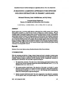
Figure 1.1: Competition between search engines: a motivating example
goog and AstiVatla having equal resource capabilities. Let us assume that users are only interested in either “sport” or “cooking”, with “sport” being the more popular topic. More specifically, let 60% of all queries relate to “sport” and the remaining 40% to “cooking”. If Elgoog and AstiVatla each decide to index documents on both “sport” and “cooking” (i.e. everything, like generic search engines try to do), they will be receiving an equal share of all user queries. If Elgoog decides to spend all its resources only on “sport” while AstiVatla stays on both topics, Elgoog will be able to provide better search for “sport” than AstiVatla. In this case, users will send queries on “sport” to Elgoog, and on “cooking” to AstiVatla. Therefore, Elgoog will be receiving more queries (and so will have higher profits). If, however, AstiVatla also decides to index only the more popular topic, both search engines will end up competing only for the “sport” queries and, thus, may each receive even less search requests than in the two previous cases. Figure 1.1 illustrates this example. The uncertainty about competitors, changes in the environment, and the potentially large number of competing engines make the task difficult. As we will see later, it turns out that naive strategies (such as “index lots of documents on popular topics”) can be highly suboptimal, because they ignore the fact that the profitability of a document depends on whether one’s competitors also index it. Decision making in this context is difficult because the competitors would be unlikely to reveal such secrets. In this thesis, we consider a scenario in which specialised search engines compete for user queries by deciding what documents (topics) to index and how much to charge users for the search services. Our research objective is to propose an approach that search engines can use to derive their competition strategies to maximise individual profits in a federated Web search environment. It is perceived that the lack of effective mechanisms for managing service parameters of individual search engines in heterogeneous search environments is one of the major obstacles for a wider deployment of such systems [Brin and Page, 1998]. We envisage that the research in this area will ultimately result in developing tools to assist services providers in decision
5
making. Note, that in this thesis we only focus on the competition between search engines based on the selection of their service parameters (i.e. topic specialisation and/or service pricing) leaving out of the scope the problems of metasearch, focused crawling, or actual query processing addressed by the prior research in distributed information retrieval (see Section 2.1.4).
1.3
Approach
To achieve our research objective, we propose to utilise knowledge and methods from three broad research areas: • information retrieval; • game theory; and • machine learning. The area of information retrieval [van Rijsbergen, 1979, Frakes and Baeza-Yates, 1992, Greengrass, 2000] provides us with the necessary knowledge about Web search engines and heterogeneous search environments. This includes the structure, functionality, and algorithms of search systems and their components as well as possible deployment and revenue generation scenarios. Game theory represents a set of sound analytical tools designed to model behaviour of independent decision makers who are conscious that their actions affect each other [Rasmusen, 1994, Petrosjan and Zenkevich, 1996, Osborne and Rubinstein, 1999]. Game theory provides a basis for strategic reasoning in the decision making process. It can also help to cope with the lack of knowledge about strategies of other decision makers in the system by making the assumption of a rational behaviour (i.e. assuming that other competing search engines are also trying to maximise their utilities). In this work, we use game theory for developing formal models of the competition process between search engines. The basic elements of game-theoretic models are players, actions available to the players, and pay-off (or utility) functions that map players’ actions onto players’ rewards. Applying this schema to federated search environments, players can represent search engines, actions are possible service parameter adjustments, and utility functions are related to the engines’ profits. One of the central problems in decision making for search engines in a heterogeneous search environment is the lack of a complete a priori information about the environment and their competitors that is necessary to determine the effects of service parameter adjustments on engines’ profits and to derive a good competition strategy. In many cases, such information can only be obtained through interaction experience. The need to be able to utilise past experience to improve future performance naturally leads us to the idea of using machine learning techniques. Machine learning [Mitchell, 1997] is a mature discipline with a rich theoretical framework and a substantial application track record. We
6
propose to use reinforcement learning [Kaelbling et al., 1996, Sutton and Barto, 1998], more specifically, multi-agent reinforcement learning [Shoham et al., 2003] which studies the problem of learning the optimal behaviour for an agent through trial and error interaction with an unknown environment in the presence of other agents. An important problem in the proposed research is how to evaluate effectiveness of candidate strategies and management algorithms. Unfortunately, evaluation using a real-life heterogeneous search environment would be very hard due to prohibitively long time frames required for capturing results in a real-life system and because of the inability to reproduce experiments. Therefore, our evaluation will rely on simulating a heterogeneous Web search environment. Obviously, to obtain competition strategies that can be applied effectively in real-life systems, the simulation must be driven by real-life workload data, and the simulation models should reflect closely properties of the corresponding real-life components. To address these issues, we use real user queries submitted to existing generic Web search engines to derive the number of submitted queries and their topical distribution in our simulations. We also propose a model of the focused Web crawling process that closely reproduces the output of real-life crawlers as reported in the literature. The advantage of simulation is that different competition strategies can be evaluated using exactly the same workloads (which would be impossible in evaluation using a real-life system), thus allowing for more precise measurements of quantitative differences between the strategies.
1.4
Contributions
This work contributes new theoretical and empirical knowledge to the area of computational economics in distributed Web information retrieval. The following list summarises our main contributions: • We present a generic formal framework modelling competition between search engines
in federated Web search environments as a partially observable stochastic game. This framework provides a formalisation of the economic issues in distributed Web search environments and can serve as a basis for future research efforts in this area.
• We provide a game-theoretic analysis of the competition in distributed Web search that
motivates the concept of “bounded rationality” [Rubinstein, 1997] and justifies the use of a heuristic machine learning solution for our problem. Bounded rationality states that decision makers are unable to act optimally a priori due to limited knowledge of the
environment and opponents, and limited computational resources. • We propose a reinforcement learning approach to deriving competition strategies for in-
dividual search engines that maximise their profits. Our approach, called COUGAR,
utilises gradient-based stochastic policy search techniques. • We provide extensive empirical evaluation results in reasonably realistic settings that show the effectiveness of the proposed approach.
7
1.5
Thesis Outline
The rest of this thesis is organised as follows: • Chapter 2 provides a brief introduction into the three main research areas employed in this work: (distributed) information retrieval, game theory, and reinforcement learning.
• Chapter 3 gives an overview of related work. Note that in this chapter we only describe studies which investigated similar economic issues of profit (or performance) maximisa-
tion in other competitive domains (i.e. not in Web search). There is also a large body of research in information retrieval, game theory, and machine learning related to this thesis. Such research is discussed in the corresponding parts focusing on game-theoretic or machine learning analysis. We believe that presentation of relevant research in context supports better understanding and minimises cross-referencing. • Chapter 4 presents a generic formal framework for modelling competition between
search engines in heterogeneous search environments and unambiguously defines our research problem in terms of this framework.
• Chapter 5 analyses the competition problem from the game-theoretic point of view and motivates the use of machine learning techniques for deriving competition strategies.
• Chapter 6 discusses the area of multi-agent reinforcement learning and describes our approach to the problem of optimal behaviour in heterogeneous Web search environments.
• Chapter 7 presents extensive empirical evaluation of the proposed approach. • Finally, Chapter 8 recapitulates contributions of this work, draws some conclusions, and outlines directions for future research.
Enjoy!
8
Chapter 2
Background In this chapter, we provide a brief introduction into the three main research areas employed in this thesis: • Distributed information retrieval; • Reinforcement learning; and • Game theory. We introduce the basic concepts and provide an overview of prior research in these areas. An additional purpose of this chapter is to introduce the corresponding terminology used throughout the rest of this thesis.
2.1
Heterogeneous Web Search Environments
In this section, we give a brief introduction into heterogeneous Web search environments, the subject of the research in this thesis. We subdivide our discussion into three parts: basics of information retrieval; description of the structure, main components, and functioning of Web search engines; and, explanation of how multiple search engines can be aggregated into a heterogeneous search environment, what the main components are there, and what functions they perform.
2.1.1
Information retrieval
Information retrieval (IR) can be loosely defined as a process of locating (i.e. establishing the existence and whereabouts of) information of interest. Since the 1940s the problem of information retrieval has attracted increasing attention. Simply stated, we have vast amounts of information to which accurate and speedy access is becoming ever more difficult. One effect of this is that relevant information gets ignored since it is never uncovered, which in turn leads to much duplication of work and effort. Traditionally, information retrieval systems operate in terms of queries and documents. A query is an expression of an information need. The particular format for expressing a query may vary. A popular choice is a set of terms, or keywords, that are supposed to describe 9
what information a user is looking for. A query is submitted to an information retrieval system, which then aims to find information relevant to the query. Relevance is an inherently subjective concept since it utterly depends on human judgements. Humans often disagree about whether a given document is relevant to a query and what is the degree of that relevance taking into consideration the user’s personal needs and expertise. The response of an information retrieval system is a set of references to documents that should satisfy the information need of the user. A document is any object carrying information: a fragment of text, an image, a sound, or a video. However, most of the current IR systems deal only with text, a limitation resulting from difficulties in representing non-textual objects. The two measures commonly used for evaluating outcomes of an IR process (based on the concept of relevance) are precision and recall. Precision can be defined as the ratio of relevant items retrieved to all items retrieved, or the probability given that an item is retrieved, it will be relevant [Saracevic, 1995]: Precision =
Relevant items retrieved . Total items retrieved
Recall can be defined as the ratio of relevant items retrieved to all relevant times in the source information storage, or the probability that given an item is relevant, it will be retrieved: Recall =
Relevant items retrieved . Total relevant items in storage
Some users pay more attention to precision, i.e. they want to see relevant documents without glancing through a lot of useless and irrelevant ones. Others pay more attention to recall, i.e. they would like to get the maximum amount of relevant documents. Therefore, an effectiveness measure where the importance of precision and recall can be specified [van Rijsbergen, 1979]: E =1−
α P1
1 , + (1 − α) R1
where α ∈ [0, 1] is the importance of precision, R is recall and P is precision. Despite some
other alternative measures proposed, TREC 1 , which is the source of the most popular IR effectiveness tests widely used in the IR research communities, utilises precision and recall measure-
ments.
2.1.2
Elements of search engines
Search engines are widely used tools for automatic information retrieval on the Web. The main function of a Web search engine is to provide a search user with URLs of Web documents relevant to a given user’s query. The activities performed by a search engine can be subdivided into the following three groups: • Discovery of Web documents. Discovery of Web documents can be performed manually
or automatically. Manual discovery requires a human to enter descriptions and URLs
1
http://trec.nist.gov
10
Web Search Engine
Web
Web crawler
Request processor
Document indexer
Document index
Search users
Figure 2.1: Components of a Web search engine
of existing Web documents. Automatic resource discovery is performed by the search engine itself by first downloading a manually specified set of starting Web pages (also called seeds) and then recursively downloading documents linked from the seeds by automatically following hyperlinks. The process of automatic Web resource discovery is usually called crawling and the search engine component responsible for it is called Web crawler or Web robot. • Processing and storage of Web documents. The goal of these activities is to extract from the retrieved Web documents information necessary for matching documents and search queries and to store these documents descriptions in a format suitable for fast and efficient search. The data structure which stores information about crawled Web pages is called document index, and the search engine component responsible for processing of Web pages and building the document index is called document indexer. • Processing of search requests. This is the main activity in a search engine. The goal of this activity is to determine for a given user search query a set of indexed Web documents
that are likely to be most relevant to the query. The size of the resulting document set may be determined by the user or automatically by the search engine, and the results are usually sorted according to their expected relevance. (Note, that we are saying here expected relevance, because relevance is a subjective characteristic and can ultimately be determined only by the user. The search engine only tries to estimate how likely it is that a document will be considered relevant by the user.) The engine component responsible for processing of search queries is called request processor or request handler. Figure 2.1 shows the typical structure of a Web search engine. The dotted link from the document index to the Web crawler symbolises the fact that besides discovering and retrieving new documents from the Web, the crawlers are also responsible for keeping information about already indexed documents up-to-date. We discussed here only a top-level structure of a search engine, the actual implementation details may vary (see for example [Brin and Page, 1998]).
11
Metasearch
Index of engines
Discovering search engines
Selecting search engines Search engine
Search users Search engine
Forwarding user queries
Web Search engine
Search engine
Merging search results
Figure 2.2: Federated (distributed) search model
2.1.3
Federated search model
Federated (also called distributed) search environments allow a user to utilise resources of multiple search engines for processing of her search requests. To achieve this, the following activities need to be performed in a federated search environment: 1. Discovery of search engines; 2. Storing and indexing information about search engines; 3. Deciding what search engines to use for every particular user search query; 4. Forwarding user queries to the selected search engines; 5. Merging search results coming from multiple engine and presenting them to the user. Figure 2.2 illustrates this federated search model. It is easy to see that the first three activities are essentially equivalent to the activities performed by a search engine, but instead of searching for documents, we search for search engines now. Hence, the components responsible for performing these functions in a federated search environment are often called metasearchers. In the simplest distributed search scenario, each user query can be forwarded to a fixed set of search engines and then the returned results merged into a single list with duplicates removed. This is the scenario implemented by some existing metasearch systems like www.dogpile.com. However, this simple scenario is only efficient if the different search engines cover random subsets of the Web with little or no overlap between them, that is, if all search engines in a federated search environment appear to be homogeneous, and there is no particular reason to choose one engine over another.
12
The main benefits of federated search environments are enabled through two key elements: engine specialisation and intelligent engine selection. Specialised search engines explicitly target only a selected subset of all resources available on the Web, thus providing a focused search service in a specific domain (e.g. on a specific topic). The goal of the engine selection process then becomes one of finding for each user query the search engines which can provide the best service for the query as measured by the quality of results, service price, and other relevant service parameters. By distributing user queries only to the search engines that are likely to provide good results, heterogeneous federated search environments essentially perform search only in a subset of the Web that is likely to contain required resources, instead of searching the whole Web for each query. This reduces the cost of providing a search service and allows for more cost-efficient and scalable Web search solutions. A typical search scenario in a heterogeneous search environment proceeds as follows: 1. The user submits its search query to a metasearcher. 2. The metasearch returns a list of search engines suitable for this query. 3. The user, manually or with help from the metasearcher, selects which engines to use for the query. 4. The query is forwarded to the selected engines. 5. The engines process the query and return lists of search results, which are collected and merged by a result merging component.
2.1.4
Distributed information retrieval
Most of the prior research work in the area of distributed information retrieval focused on the three main technical aspects of the federated heterogeneous search environments: building of topic-specific search indices (focused crawling), selection of search engines, and merging of search results. Focused crawling For a generic search engine, any document found by a Web crawler is equally valuable. This is not the case for a specialised search engine which is only interested in documents that fit within the scope of its specialisation (i.e. belong to a specific topic). Since downloading and analysing Web documents involves the corresponding computational and network costs, the goal of a topic-specific (or focused) Web crawler is to minimise the number of downloaded off-topic documents, while maximising the number and relevance of on-topic documents. Therefore, while for a generic crawler is does not matter in what order to explore the hyperlinks from already downloaded pages (i.e. in what order to traverse the Web graph), a focused crawler should attempt to schedule document downloads to obtain the on-topic documents as soon as possible, given the restrictions imposed by the Web connectivity. 13
There are two basic methods of automatically populating a topic-specific document index which can be referred to as cooperative and independent crawling. Cooperative crawling occurs when non-topic-specific robots are used to create a centralised pool of document descriptions which are then shared by all of the participants in a federated search system. Topic-specific search engines can then be created by selecting documents descriptions from the shared pool in a topic sensitive manner. The cooperative crawling approach has been employed by existing distributed search systems such as Harvest [Bowman et al., 1995]. In the case of independent crawling, each participant independently constructs their own topic-specific search index. The techniques employed in this field can be broadly categorised as either heuristic or machine learning based. Early topic-specific robot algorithms were heuristic based. Examples of these early systems include the Fish-Search algorithm and the WebCrawler [Bra and Post, 1994, Pinkerton, 1994]. More recent examples of heuristic algorithms include the Shark-Search algorithm, the Focused Crawler, and the OASIS Crawler [Hersovici et al., 1998, Nekrestyanov et al., 1999, Chakrabarti et al., 1999]. These systems use heuristics of varying complexity but all employ one or more of the following assumptions: the content of a child page tends to be similar to that of its parent pages 2 ; the similarity of sibling pages increases when links on a parent page are close together; and that anchor text is similar to its target page. A recent study has empirically validated these assumptions [Davison, 2000]. Heuristic focused crawling algorithms provide reasonable though limited levels of performance. Their limitations stem from their inability to adapt to system inputs and the fact that they are not based on a solid model of the problem they are trying to solve. There is no obvious heuristic approach to take “rapid fire” requests 3 into account for example. Adaptive algorithms based on machine learning approaches can improve their performance based on the system inputs and consequently have at least the potential to achieve closeto-optimal performance. The examples of adaptive algorithms related to the topic-specific robot problem include the InfoSpiders and Cora Spider algorithms [Menczer and Belew, 2000, McCallum et al., 2000] The InfoSpiders algorithm uses an ecological model of distributed agents following paths through the Web graph [Menczer and Belew, 2000]. A distributed evolutionary algorithm and representation was used to construct populations of adaptive agents. Each agent used a reinforcement learning algorithm (see Section 2.2 for an introduction into reinforcement learning) to train a neural network to predict which links to follow so as to maximise the reward gained (where the reward was a function of the relevance of the documents retrieved). Reinforcement learning has been used to solve problems of deriving a behaviour in an environment modelled by a state based system (such as Markov Decision Process, see Section 2.2 2
A parent page contains a link to a child page. While Web crawlers essentially reproduce the behaviour of humans browsing Web pages, they can issue download requests much more frequently than humans. This may result in overloading Web sites with too many page requests, a problem known as “rapid fire” requests. To avoid overloading, most Web sites limit the number of download requests from a given source that can be served per some time unit. Consequently, Web crawlers have to schedule download requests to take into account such restrictions. 3
14
for more details). Reinforcement learning algorithms use trial-and-error experience to estimate the value of taking an action in a given state of the system. The value of an action in a given state is a sum of the immediate reward and the expected subsequent rewards that results from taking that action. By modelling the problem as one of following a path through a graph, InfoSpiders applied an existing reinforcement learning algorithm, Q-learning (see Section 2.2.4), by simply mapping states to documents and actions to following links. This model, however, does not (and was not intended to) directly solve the topic-specific Web robot problem. In InfoSpiders, an agent can only request a child document of the last document it retrieved. In the Web crawling problem, the requested document can be a child of any document previously retrieved. In addition, InfoSpiders did not incorporate the avoidance of “rapid fire” requests into its model. The designers of the Cora Spider algorithm also employed reinforcement learning techniques but recognised the limitations of the InfoSpiders model [McCallum et al., 2000]. Instead of using a “paths through the graph” model, where the state is the last document retrieved, they realised that the state actually consists of the set of retrieved documents. The action space then consists of the set of requestable documents. Unfortunately, this realisation is of little assistance in solving the problem as the state-action space is exponential in the number of documents for most Web graphs of interest. To resolve this, Cora Spider first solves the problem off-line for a known graph of documents under a set of simplifying assumptions, and then trains a function approximator (a regression function in this case) with the solution. The generalisation abilities of the approximator are then used to generalise the solution to unknown document graphs on-line. Search engine selection To process search queries in a heterogeneous search environment, it is necessary to be able to find out for each query what specialised search engines in the system can provide relevant results. To achieve this, engine selection algorithms need to know what each search index contains. This information is often derived from a unigram language model, which lists the words that occur in the indexed documents and their frequencies of occurrence. [Gravano and Garcia-Molina, 1999] proposed bGlOSS and vGlOSS as an approach for the boolean and vector information retrieval models [Salton and McGill, 1983]. gGlOSS is a generalisation of the previous two GlOSS models to any vector-based information retrieval approach that computes a score to determine how well a document satisfies a query, provided that certain index statistics are made available to gGlOSS. Under vector-space model, documents are represented as vectors. If m distinct words are available for content identification, a document d is represented as a normalised m-dimensional vector, D = (w1 , . . . , wm ), where wj is the weight assigned to the j th word tj . If tj is not present in the document, then wj is 0. The weight for the document word indicates how statistically important it is and is computed based on the frequency of occurrence of this word in the document (term frequency) and the popularity of the word in the whole search index (i.e. the number of documents containing this word – document frequency). Using the document
15
frequency takes into account the content discriminating power of the word: a word that appears rarely in documents has a higher weight than a word that occurs in many documents. Each search index is then is described by two vectors: • A vector of document frequencies containing the number of documents with a given term in the index; and • A vector of term weights, in which each element is the sum of the weights of a given term over all the documents in the index.
These two vectors are used to estimate how good a search index is for processing of a given user query. The main idea behind the estimation algorithm is that if the search engine contains many documents with the terms appearing in a user query, then this engine is likely to be good for processing this query. The actual algorithm computes a score for each search index, so that search engines could be ranked by their suitability for processing of a given search request. [Callan et al., 1995] proposed an engine selection method based on inference network information retrieval model called collection retrieval inference network, or CORI network. The Inference Network Model (INM) is an approach to applying conditional probability in information retrieval. It can simulate both probabilistic and Boolean queries and can be used to combine results from multiple queries, as well as multiple sources of evidence. The documents in INM can be represented by automatically extracted terms from the documents or terms (concepts) assigned manually. A typical probabilistic information retrieval model computes the probability that user decides the document is relevant to the user’s query (see also Section 4.3.1). The INM computes Pr(Information need |Document), the probability that particular document would sat-
isfy user’s information need. This probability can be computed separately for each particular
document in a search index. Multiple approaches were implemented to calculate the probabilities in INM [Turtle and Croft, 1991, Greiff et al., 1997], which mainly tended to decrease the amount of computing resources used to operate in INM. The CORI network algorithm developed by [Callan et al., 1995] is based on the document retrieval inference network method described by [Turtle and Croft, 1991]. [Craswell et al., 2000] proposed a method for estimating relevance of search engines by sending probe queries and analysing results. The problem of estimating relevance of document collections via probe queries was also addressed in [Meng et al., 1999]. Other examples of engine selection algorithms include CVV (Cue-validity Variance) [Yuwono and Lee, 1996] and CSams [Wu et al., 2001], a selection method and a prototype metasearch engine for computer science academic metasearch. Earlier works on routing search queries to the appropriate search services include Sheldon’s dissertation on content routing [Sheldon, 1995] and the Discovery project which uses content routing and query refinement techniques to search a large number of WAIS servers [Sheldon et al., 1995].
16
Result merging Each search engine involved in processing of a given search request produces a list of search results ranked by their expected relevance to the query. The main problem for result merging is to aggregate these results into a single list while preserving the relevance ordering. Existing research [Voorhees, 1995, Craswell et al., 1999] identifies two basic categories of merging strategies. The distinction between the two groups is based on whether merging information is provided by the search engines. [Craswell et al., 1999] classifies these approaches as: • integrated merging methods; and • isolated merging methods. In the case of integrated merging, search engines use system-wide statistics (i.e. common information regarding all search engines in a heterogeneous environment) in conjunction with a uniform ranking algorithm to assign each document a relevance score. The main advantage of this methodology is that it allows each search engine to compute document scores that are directly comparable with the document scores generated by the other engines in the system. Isolated merging mechanisms are based on locally assigned relevance scores (i.e. on the relevance scores assigned by search engines using only information about their own indices). These scores are not directly comparable: even if all engines use the same ranking algorithm, they will still be using local index statistics (e.g. document frequencies) that are only relevant to that particular search engine. As a result, some manipulation of the local scores is necessary to sort the documents in a merged result list. Examples of operations that can be carried out to accomplish this balancing process range from scaling the scores so that they fall between two set values [Selberg and Etzioni, 1995], to assigning preferences to documents from engines that are deemed to be more useful [Gauch et al., 1996]. Distributed search systems and architectures Apart from addressing separate technical aspects of federated search environments (such as focused crawling, engine selection, or result merging), a number of research projects focused on incorporating these techniques into prototype or even commercial distributed search systems. Below, we describe several representative examples of such efforts. OASIS is a distributed search system, providing search services for plain text and HTML documents stored on publicly accessible Web and FTP servers [Patel et al., 1999]. An OASIS server consists of the following components: a query server that manages distributed query processing; zero or more topic-specific collections that contain and search indices on specific topics; zero or more Web crawlers. The query server plays a central role in the OASIS architecture. Its responsibilities include query propagation to a set of collections (i.e. metasearch) and merging or search results. An OASIS collection essentially provides services of a topic-specific Web search engine. The OASIS crawler can be used to construct and maintain an OASIS collection. The crawler’s goal is to maximise the relevance of the documents in its collection with respect to the collection’s topic specialisation. It employs a subject-specific harvesting strategy 17
to decide which documents on the Web to retrieve for inclusion in the collection and which documents to revisit to ensure the collection remains up-to-date. Inter-crawler communication allows one crawler to recommend a URL to another crawler in the OASIS system. The Harvest system [Bowman et al., 1995] was originally developed in 1995 as part of the ARPA-funded Harvest project. Development of the system now continues at the University of Edinburgh. The goal of Harvest is to provide an integrated set of customisable tools for gathering information from diverse repositories, building, searching, and replicating content indices, and caching retrieved objects. The system has the following types of components: • A Gatherer collects and extracts information from one or more Providers (such as Web of FTP servers). For example, a gatherer can collect PostScript files and extract text from them, or it can extract subjects and author names from USENET archives and so on. • A Broker provides the indexing and the query interface to the gathered information. Brokers retrieve information from one or more gatherers or other brokers, and incrementally update their indices. Harvest includes a distinguished broker called the Harvest Server Registry (HSR), which allows users to register information about each Harvest gatherer, broker, cache, and replicator in the Internet. • A Replicator can be used to replicate servers: for example, the HSR will likely become heavily replicated. The replication subsystem can also be used to divide the gathering
process among many servers, distributing the partial updates among the replicas. • An Object Cache reduces network load, server load, and response latency when accessing located information objects.
The Harvest Broker consists of four software modules: the Collector, the Registry, the Storage Manager and Index/Search Engine, and the Query Manager. The Registry and Storage Manager maintain the authoritative list of summary objects that exist in the Broker. The Collector periodically requests updates from each gatherer or broker specified in its configuration file. The Query Manager exports objects to the network. It accepts a query, translates it into an intermediate representation, and then passes it to the search engine. MetaCrawler4 [Selberg and Etzioni, 1995] operated at the University of Washington from 1995 to 1997. MetaCrawler provided a single, central interface for World Wide Web document searching using multiple search services. Upon receiving a query, MetaCrawler posted the query to multiple generic search engines in parallel, and performed pruning on the responses returned. More specifically, the MetaCrawler collates the results by merging all hits returned. Duplicates are listed only once, but each service that returned a hit is acknowledged. Optionally, the MetaCrawler can verify the information’s existence by downloading the references. When the MetaCrawler has loaded a reference, it is then able to re-score the page using supplementary query syntax supplied by the user. In particular, the user can specify required and non-desired words, as well as words that should appear as a phrase. Also, expert options allow users to rank hits by physical location, such as the user’s country, as well as logical locality, such as their 4
http://www.metacrawler.com
18
Internet domain. Experiments indicated that MetaCrawler was able to prune as much as 75% of the returned responses as irrelevant, outdated, or unavailable. MetaCrawler received upwards of 60,000 queries daily, making it one of the most popular meta-searching services in the world while operated by the University of Washington. Go2Net, now InfoSpace, took over exclusive operation of MetaCrawler in 1997. SavvySearch5 [Howe and Dreilinger, 1997] ran at Colorado State University from March 1995 until its acquisition by CNET. Probably the most prominent feature of SavvySearch is that it learns which search engines to query, using simple AI techniques. SavvySearch is designed to balance two goals: maximising the likelihood of returning good links and minimising computational and Web resource consumption. The key to compromise is knowing which search engines to contact for specific queries at particular times. SavvySearch tracks long term performance of search engines on specific query terms to determine which are appropriate and monitors recent performance of search engines to determine whether it is even worth trying to contact them. SavvySearch queries many different types of Internet resources, including: search engines; classified directories (e.g., Yahoo!); Usenet; shareware (e.g., Tucows); e-mail addresses; newspapers (e.g., New York Times); encyclopaedias; movies (e.g., Internet Movie Database). The user has to choose a particular type of resources for her query. When querying search engines or classified directories, SavvySearch supports phrase searching, enforced term operators (+/−), Boolean operators (AND, OR, NOT) and associativity grouping using round brackets.
2.2
Reinforcement Learning
The history of reinforcement learning goes back to the early days of cybernetics and computer science. Lately, it has attracted considerable interest in the machine learning and artificial intelligence communities. Summarised in one sentence, the idea of reinforcement learning is to provide a way of programming agents to perform some task by rewarding and punishing them, but without needing to specify how the task should be achieved. More precisely, reinforcement learning is the problem faced by an agent that must learn behaviour through trial-and-error interaction with a dynamic environment. In this section, we provide a brief introduction into reinforcement learning, and describe the concepts and algorithms important for understanding the rest of this thesis. For a detailed introduction see for example [Sutton and Barto, 1998]. The discussion in this section follows closely the survey by [Kaelbling et al., 1996].
2.2.1
Reinforcement learning model
The standard reinforcement learning model consists of the two main components: a learning agent and a dynamic environment. The agent is connected to its environment via perception and action signals as shown in Figure 2.3. The interaction with the environment proceeds in steps. At each step, the agent receives as input some indication o (observation) of the current state s of the environment and then gener5
http://www.savvysearch.com
19
Environment Environment state
Transition function
Action Observation function Reward function
Observation Behaviour policy Reward
Agent
Figure 2.3: Reinforcement learning model
ates an output by choosing some action a. The action changes the state of the environment, and the value of this state transition is communicated back to the agent using some scalar reinforcement signal r. The interaction between the agent and the environment can be demonstrated by the following example dialog from [Kaelbling et al., 1996]: Environment: You are in state 65. You have 4 possible actions. Agent: I will take action 2. Environment: You receive a reinforcement of 7 units. You are now in state 15. You have 2 possible actions. Agent: I will take action 1. Environment: You receive a reinforcement of −4 units. You are now in state 65. You have 4 possible actions. Agent: I will take action 1. ... The goal of the agent is to find a decision rule (a policy) that maximises some long-term measure of the reinforcement. In general, the environment can be non-deterministic, i.e. taking the same action in the same state may result in different state transitions and/or reinforcements. However, it is usually assumed that the environment is stationary. That is, the probabilities of making state transitions or receiving specific rewards do not change over time. There are several differences between reinforcement learning and the more widely studied problem of supervised learning [Mitchell, 1997]. The most important difference is that there is no presentation of the optimal input-output pairs. After choosing an action, the agent is told the immediate reward and the next state, but it is not told the action that would have been best (optimal) in its long-term interests. Another difference is that the performance during learning may also be important, i.e. the evaluation of the system may be concurrent with learning. Formally, the agent’s environment is well modelled as a Markov Decision Process (MDP). 20
Definition 2.1. A Markov Decision Process (MDP) is a tuple hS, A, R, T i, where • S is a set of the environment states. • A is a set of actions available to the agent in each state. • R:S×A→
is a reward (reinforcement) function.
• T : S × A × S → [0, 1] is a state transition function that maps a given pair (s, a) of state and action onto a probability distribution over the next states.
It is usually assumed that the state and action sets are finite. Therefore, T (s, a, s 0 ) is the probability that after performing action a in state s, the next state of the MDP will be s 0 . A policy of an agent in reinforcement learning is in general a function Λ that maps sequences of past observations of the MDP states (i.e. agent’s inputs) onto distributions over the agent’s actions: Λ : O × A → [0, 1], where O is a set of possible observation sequences of the agent. If the mapping is deterministic (i.e. Λ ∈ {0, 1}) then the policy is called deterministic.
From the agent’s point of view, there are two types of environments: Fully observable
environments and partially observable environments. In fully observable environments, the agent can reliably observe the exact state of the environment at each step. In partially observable environments, the agent may not be able to distinguish between some state of the environment based on its observations. The formal model describing partially observable environments is called partially observable MDP (POMDP). To account for partial observability in a POMDP, an observation function is used. An observation function Ω in a POMDP is a partition of the set of the environment states S. Ω maps the set of all possible states S to a set of all possible observations O of the agent. For every
K state sequence s = (sk )K k=1 , sk ∈ S, there is an observation sequence o = (o k )k=1 , ok ∈ O
of the agent, where ok = Ω(sk ) is an observation at step k. In particular, for fully observable MDPs Ω(s) = s. In the further discussion, whenever we do not explicitly mention the type of the environ-
ment, we refer to a fully observable environment. For example, when we talk about learning a policy in an MDP, we will mean a fully observable MDP.
2.2.2
Notions of optimality in reinforcement learning
Since during interaction with its environment an agent can receive multiple reinforcements (rewards), it is important to define how these separate rewards are incorporated into a long-term performance measure. Let (rk )K k=1 be a sequence of rewards received by the agent over K steps of interaction with the environment. There are several ways to calculate the long-term reward for a given sequence of rewards from separate steps. The most widely used ones are the following: • Discounted sum: The long-term reward of the agent is evaluated as a discounted sum of
21
rewards received at each separate step: K � X U (rk )K = γ k−1 rk , k=1 k=1
where rk is the reward received at step k, and 0 < γ ≤ 1 is a discount factor. A special
case of this method is γ = 1, when the long-term performance is evaluated simply as a
sum of all stage rewards received. • Average reward: The long-term reward of the agent is evaluated as an average reward over all game stages played:
K � 1 X = U (rk )K rk , k=1 K k=1
where, similarly to the previous case, r k is the reward of the agent at stage k. Theoretically, the interaction of the agent with the environment may continue over infinite number of steps. The case when the interaction is analysed over a infinitely many steps is called the infinite horizon model, as opposed to a finite number of step in the finite horizon model. The long-term payoff in the infinite horizon case is evaluated as a limit for K → ∞: � K U ((rk )∞ k=1 ) = lim U (rk )k=1 . K→∞
The infinite-horizon discounted sum model has received the most attention in reinforcement learning due to its mathematical tractability. These criteria for assessing reward sequences of an agent in reinforcement learning can be used to evaluate the performance of a learned policy. However, since the environment transitions can be non-deterministic, the same policy may result in different long-term rewards over different interaction sequences. Therefore, the quality of a policy is evaluated as the expected long-term reward for the selected evaluation criterion. For example, for the infinite-horizon discounted sum, the policy’s performance is evaluated as U (Λ) = EΛ
∞ X k=1
γ k−1 rk
!
.
The policy is called optimal if it yields the maximum possible expected long-term reward for the chosen evaluation model in a given MDP. In addition to assessing the quality of a learned policy, one may also wish to evaluate the quality of the learning process itself. Several measures are in use: • Eventual convergence to the optimal policy Many reinforcement learning algorithms come with a provable guarantee of asymptotic convergence to the optimal behaviour.
22
However, as pointed out
in [Kaelbling et al., 1996], this property may not be much useful in practice. An algorithm that quickly reaches 99% of the optimal performance may be more useful in practice than an algorithm that is guaranteed to eventually reach the optimal policy, but yields poor performance in the early learning stages. • Speed of convergence to optimality This measure specifies the amount of learning interactions required for an algorithm to converge to the optimal or to a near-optimal policy. This measure also has drawbacks. For example, an algorithm that quickly converges to the optimal policy may result in high performance penalties during the learning period, and may be less desirable than an algorithm that takes longer to converge but achieves a greater performance during learning (recall the differences between supervised learning, Section 2.2.1). • Regret Regret is the expected decrease in the long-term reward due to executing the learning algorithm instead of using the optimal policy from the very beginning. This measure penalises mistakes whenever they occur during the interaction. Unfortunately, results concerning the regret of algorithms are hard to obtain [Berry and Fristetd, 1985].
2.2.3
Computing a policy given a model
Many reinforcement learning algorithms take their inspiration in the dynamic programming techniques [Bertsekas, 1995] that are used to solve the problem of finding the optimal policy for an agent given an MDP model of the agent’s environment. Here we will restrict our analysis to infinite-horizon discounted model of long-term rewards, because it is the most widely used in reinforcement learning. However, most of these techniques have analogs for average-reward and finite-horizon models. Let V ∗ (s) = max EΛ Λ
∞ X
!
γ k−1 rk (s) ,
k=1
where rk (s) is the agent’s reward at step k after staring in state s, be the optimal value of state s. The value of state s can be viewed as the expected long-term performance of the optimal strategy under the infinite-horizon discounted-sum criterion in the the given MDP that starts in state s. This state value function is unique and can be defined as a solution to a system of Bellman equations [Bellman, 1957]: ∗
V (s) = max R(s, a) + γ a∈A
X
s0 ∈S
0
∗
0
!
T (s, a, s )V (s ) , ∀s ∈ S,
which essentially states that the value of a state is the sum of the immediate reward and the expected discounted value of the next state, using the best available action. Given the optimal
23
state value function, the optimal behaviour policy can be specified as a deterministic policy Λ∗ (s) = arg max R(s, a) + γ a∈A
X
!
T (s, a, s0 )V ∗ (s0 ) .
s0 ∈S
(2.1)
The policy that depends only on the current state (or state observation), but not on the history of past state observations is called Markov (or reactive). Therefore, every fully observable MDP has an optimal deterministic Markov policy. There are two principal ways to find the value function (i.e. to solve the Bellman equations): value iteration and policy iteration. The value iteration algorithm is shown in Figure 2.4. for all States s do Initialise V (s) arbitrary end for repeat for all States s do for all Actions a do P Q(s, a) = R(s, a) + γ s0 ∈S T (s, a, s0 )V (s0 ) end for V (s) = maxa∈A Q(s, a) end for until Policy is good enough Figure 2.4: Value iteration algorithm
The Bellman residual [Bellman, 1957] of the current value function can be used to derive a stopping condition for value iteration. Bellman residual says that if the difference between two successive value functions is less than �, then the performance of the greedy policy (i.e. the policy obtained by choosing in every state the action that maximises the expected longterm reward given the current estimate of the state values) differs from the performance of the optimal policy by no more than 2�γ/(1 − γ) at any state.
Value iteration is very flexible. In particular, the assignments to V (s) need not happen
in the strict order as defined in Figure 2.4, but can happen asynchronously provided that the value of each state gets updated infinitely often on an infinite run. It can also be shown (see e.g. [Singh, 1993]) that updates of the form �
0
0
�
Q(s, a) = Q(s, a) + α r + γ max Q(s , a ) − Q(s, a) , 0 a ∈A
(2.2)
can be used instead as long as each pairing of s and a is updated infinitely often, s 0 is sampled from the distribution T (s, a, s0 ), and r is sampled with mean R(s, a) and bounded variance, and the coefficient α is decreased (appropriately) slowly. This type of sample backup (or update, as opposed to full backups in Figure 2.4) is crucial for operation of many learning algorithms. The second principal method for finding the value function is policy iteration. The corresponding algorithm is presented in Figure 2.5. For the obtained optimal policy, one can calculate the optimal value function. Therefore,
24
Choose an arbitrary policy Λ0 (s) repeat Λ(s) = Λ0 (s) P Solve the linear equations: V (s) = R(s, Λ(s)) + γ s0 ∈S T (s, Λ(s), s0 )V (s0 ) for all States s do P Improve policy: Λ0 (s) = arg maxa∈A (R(s, a) + γ s0 ∈S T (s, a, s0 )V (s0 )) end for until Λ(s) = Λ0 (s) ∀s ∈ S Figure 2.5: Policy iteration algorithm
value iteration works by producing successive approximations of the value function, while policy iteration produces successive improvements to the policy until it reaches the optimum. For a discussion of the computational complexity and required number of iterations of the algorithms see [Kaelbling et al., 1996].
2.2.4
Learning in fully observable domains
Reinforcement learning is primarily concerned with how to obtain the optimal policy when the model of the environment is not known. That is, the agent does not know in advance the reward and state transition functions R and T . The agent has to interact with the environment to obtain this information and, using some algorithm, process it to derive an optimal policy. Two possible approaches can be suggested here: • Model-free: Learn a policy without learning a model of the environment; and • Model-based: First learn a model of the environment and then use it to derive the optimal policy.
In this section, we will briefly describe example algorithms from both classes. The choice of the algorithms here is mainly motivated by a subsequent discussion Chapter 6. For a more representative survey, see [Kaelbling et al., 1996]. Model-free learning Q-learning [Watkins, 1989, Watkins and Dayan, 1992] is a well-known and popular model-free reinforcement learning algorithm. Let Q ∗ (s, a) be the expected discounted long-term reward from taking action a in state s and then continuing by choosing actions optimally. In this case, the value of state s can be defined as V ∗ (s) = maxa∈A Q∗ (s, a). Taking this into account, we obtain the following: Q∗ (s, a) = R(s, a) + γ
X
s0 ∈S
T (s, a, s0 ) max Q∗ (s0 , a0 ). 0 a ∈A
Also, from Equation 2.1, we obtain that the optimal policy can be found as Λ ∗ (s) = arg maxa∈A Q∗ (s, a).
25
Because the Q-function makes the action explicit, we can estimate Q-values during learning using the update rule based on Equation 2.2. Namely, after performing action a in state s, receiving reward r, and observing the next state s 0 during learning, the following update is performed: �
0
0
�
Q(s, a) = Q(s, a) + α r + γ max Q(s , a ) − Q(s, a) . 0 a ∈A
If each action is executed in each state infinitely often on an infinite run, and α is decreased appropriately, then the Q-values will converge with probability 1 to the correct values Q∗ [Watkins, 1989, Tsitsiklis, 1994, Jaakkola et al., 1994a]. The algorithm is presented in Figure 2.6. Initialise α for all State and action pairs (s, a) do Initialise Q(s, a) arbitrary end for loop In the current state s choose action a = arg max a∈A Q(s, a) with some exploration (i.e. sometimes choose a randomly) Execute action a Receive immediate reward r and observe the next state s 0 Q(s, a) = Q(s, a) + α (r + γ maxa0 ∈A Q(s0 , a0 ) − Q(s, a)) Decrease α appropriately end loop Figure 2.6: Q-learning algorithm
When the Q-values nearly converged to their optimal values Q ∗ it is appropriate for the agent to act greedily (i.e. to always choose actions with the highest Q-values). Early in the learning process, however, a difficult trade-off needs to be made between exploitation (acting greedily) and exploration (choosing non-greedy actions). An advantage of Q-learning is that it is exploration insensitive. It will converge to the correct Q-values independently of the exploration policy as long as each state-action pair is tried often enough. Thus, the standard practice is to adopt various ad hoc approaches to the exploration problem. Other model-free algorithms include TD(0) and TD(λ) [Sutton, 1988]. Model-based learning An example of a model-based algorithm is Dyna [Sutton, 1991], which actually exploits a middle ground between model-free and model-based approaches. It simultaneously uses the interˆ uses experience to adjust the policy, and uses the action experience to build a model ( Tˆ and R), model to adjust the policy. The algorithm is presented in Figure 2.7. The Dyna algorithm requires k times the computation effort of Q-learning per iteration. However, in many cases it requires an order of magnitude fewer interaction steps than does Q-learning to converge to an optimal policy. Other model-based algorithms include Prioritised Sweeping and Queue-Dyna [Moore and Atkeson, 1993, Peng and Williams, 1993].
26
Initialise α for all State-action pairs (s, a) and state transitions (s, a, s 0 ) do Initialise Q(s, a) arbitrary ˆ a) arbitrary Initialise R(s, ˆ Initialise T (s, a, s0 ) arbitrary end for loop In the current state s choose action a = arg max a∈A Q(s, a) with some exploration (i.e. sometimes choose a randomly) Execute action a Receive immediate reward r and observe the next state s 0 ˆ Tˆ ) by incrementing statistics for state transition (s, a, s 0 ) and Update the model (R, received reward (s, a, r) ˆ a) + γ P 0 Tˆ (s, a, s0 ) maxa0 ∈A Q(s0 , a0 ) Update the policy: Q(s, a) = R(s, s ∈S for k additional updates do Choose randomly (sk , ak ) P 0 0 0 ˆ k , ak ) + γ ˆ Q(sk , ak ) = R(s s0 ∈S T (sk , ak , s ) maxa0 ∈A Q(s , a ) end for end loop Figure 2.7: Dyna algorithm
2.2.5
Learning in partially observable domains
The most naive approach to dealing with partial observability is to ignore it. In this approach, observations are treated as if they were states of the environment, and the agent is trying to learn an optimal policy in the same way as in a fully observable MDP. However, since different environment states can map into the same observations, it simply may not be possible to implement the optimal behaviour using deterministic Markov policies. The learning algorithms for fully observable domains are not guaranteed to converge in POMDPs, since from the algorithm’s point of view, the environment is non-Markovian. If we associate observations with states, the reward and state transition probabilities for such “observation states” appear non-stationary, since they are generated by different actual states of the environment. Moreover, finding the best deterministic Markov policy is NPhard [Littman, 1994b], and even the best such policy can have very poor performance. Some improvement can be gained by considering stochastic Markov policies. The randomness in the agent’s actions may allow it to improve performance by acting differently for the same observations. [Jaakkola et al., 1994b] proposed an algorithm for finding locally-optimal stochastic Markov policies, but finding a globally optimal such policy is still NP-hard. To be able to distinguish between environment states for the same observation, the agent needs to use the history of past observations. Theoretically, the optimal policy in a POMDP may need to depend on infinitely long past observation sequences. Therefore, the problem of finding such a policy is intractable in general. As a result, most approaches to learning in POMDPs concentrated on learning a possibly sub-optimal policy. One way to do it is to use restricted policies (i.e. belonging to some class of policies) and try to learn the best policy in the chosen class. This method is also known as policy 27
Reinforcement learning algorithms
Fully observable environments (MDPs)
Model−based
Dyna Prioritised sweeping
Partially observable environments (POMDPs)
Model−free
Model−based
Model−free
Q−learning TD(0), TD( λ)
Learning in belief−state MDP
Policy search
Figure 2.8: Taxonomy of reinforcement learning algorithms
search (a more detailed discussion of policy search algorithms will follow in Section 6.2.4. The already mentioned algorithm by [Jaakkola et al., 1994b] is an example of this approach based on stochastic Markov policies. Other examples use policies with internal memory that can keep some information about past observations (e.g. a finite window of past observations) [Lin and Mitchell, 1992]. Another way is to use algorithms for fully observable MDPs, but to couple them with some state estimation device. The purpose of such state estimation device is to derive the expected state of the environment (also called belief state) based on the past observations. Hidden Markov model (HMM) techniques [Cassandra et al., 1994] can be used to learn the model of the environment for the state estimation. Then the goal of the reinforcement learning algorithm would be to learn the optimal policy in the belief state space.
2.2.6
Classification of reinforcement learning algorithms
In this section, we summarise the discussion on the existing reinforcement learning algorithms by providing a simple algorithms taxonomy in Figure 2.8. All algorithms are classified into two large groups depending on the type of the problem domain – fully or partially observable environments. In each group, there are two sub-classes for model-based and model-free algorithms.
2.3
Game Theory
Game theory is a set of analytical tools designed to model the behaviour of interacting decision makers. The basic assumptions that underlie the theory are that decision makers: • pursue well-defined objectives; and • take into account their knowledge and expectations of the behaviour of other decision makers.
28
The first assumption essentially tells us that the decision makers are rational (informally speaking, use some consistent and logical thinking in their decisions). The second assumption tells us that they reason strategically. A game is a description of strategic interaction between decision makers, referred to as players in the game. A game specifies constraints on the possible players’ behaviours (i.e. tells what players can do), but does not specify what action they do take. A solution is a description of the outcomes that may emerge in a game. The goal of game-theoretic studies is usually to suggest reasonable solutions and examine their properties. There are two branches of game theory: non-cooperative and cooperative. The noncooperative game theory treats actions of individual players as primitives and focuses on what individual players can achieve. In contrast, cooperative game theory treats actions for groups of players (coalitions) as primitives and concentrates on what outcomes can be achieved by coalitions. To illustrate the difference between non-cooperative and cooperative models, we borrow the following example from [Osborne and Rubinstein, 1999]. A group of individuals has a set of inputs and a set of technologies for producing a valuable single output. Each individual’s inputs are unproductive in his own technology, but productive in some other individual’s technology. A non-cooperative model of this situation would consider actions available to each individual. For instance, individuals can trade their inputs between each other. By contrast, a cooperative model looks at the set of outcomes that each possible group of individuals can jointly achieve (cooperating with each other), but does not consider the questions of how such coalitions can be sustained. Cooperative models assume the possibility of binding agreements between players in a coalition: actions of each individual player are prescribed by a common interest of the coalition. This thesis focuses exclusively on non-cooperative game theory. In particular, the term “game” in the remaining part of this section refers to a non-cooperative game. The purpose of this section is to briefly review the basic elements of non-cooperative game theory that are relevant to this thesis, and introduce the corresponding terminology, used in a subsequent analysis. For a more detailed introduction into game theory see [Osborne and Rubinstein, 1999].
2.3.1
Normal-form games
Normal-form games represent the simplest game models. A normal-form game is a model of interactive decision making in which each decision maker chooses his plan of action once and for all, and these decisions are made simultaneously. A normal-form game can be represented by a tuple hI, (A i )Ii=1 , (�i )Ii=1 i where • I is the number of players in the game. • For each player 1 ≤ i ≤ I, Ai is a non-empty set of actions available to player i. • For each player 1 ≤ i ≤ I, �i is a preference relation on the set of possible joint actions of all players A = A1 × A2 × · · · × AI .
29
The current convention in game theory is that the preference relation � i of each player i
satisfies the assumption from [von Neumann and Morgenstern, 1944] that it can be represented by a utility or payoff function ui : A →
, such that for any a ∈ A and b ∈ A, u (a) ≥ i
ui (b) if and only if a �i b. The values of this function are called player’s payoffs or utilities. Consequently, we will use the following definition of a normal-form game:
Definition 2.2. (Normal-form game) A normal-form game is a tuple hI, (Ai )Ii=1 , (ui )Ii=1 i where • I is the number of players in the game. • For each player 1 ≤ i ≤ I, Ai is a non-empty set of actions available to player i. • A = A1 × A2 × · · · × AI is the set of all possible joint actions (or action profiles) of players.
• For each player 1 ≤ i ≤ I, ui is a utility function ui : A → . If the action sets Ai are finite for each player i, then the game is called finite. A finite normal-form game in which there are only two players can be conveniently described by a table or a matrix (see Table 2.1). Actions of one player are identified with rows (the row player), and actions of the other player are identified with columns (the column player). Each element of the matrix specifies payoffs of both players for the corresponding joint action. Such games are also called matrix games. Table 2.1: A matrix game
r1 r2
c1 ur (r1 , c1 ), uc (r1 , c1 ) ur (r2 , c1 ), uc (r2 , c1 )
c2 ur (r1 , c2 ), uc (r1 , c2 ) ur (r2 , c2 ), uc (r2 , c2 )
Pure strategy Nash equilibrium The most commonly used solution concept in game theory is that of Nash equilibrium [Nash, 1950a]. A Nash equilibrium captures a steady state of the play of a normal-form game in which each player holds correct expectations about the other players’ behaviour and acts rationally (i.e. maximises its payoff with respect to its expectations). Let a = (ai )Ii=1 be an action profile of players in a normal-form game. We use a −i to denote an action profile of all players except i: a −i = (a1 , a2 , . . . , ai−1 , ai+1 , . . . , aI ). Let A−i be the set of all such action profiles: A −i = A1 × A2 × · · · × Ai−1 × Ai+1 × · · · × AI . An action profile a can be represented as (a i , a−i ).
Definition 2.3. (Pure strategy Nash equilibrium of a normal-form game) A pure strategy Nash equilibrium of a normal-form game hI, (A i ), (ui )i is an action profile
a∗ ∈ A such that for every player 1 ≤ i ≤ I
ui (a∗i , a∗−i ) ≥ ui (ai , a∗−i ) 30
for all ai ∈ Ai . That is, for an action profile a∗ to be a pure strategy Nash equilibrium, no player i must have an action ai that yields a higher outcome than a∗i when all other players j choose their equilibrium actions a∗j . Briefly, no player has an incentive to unilaterally deviate from the equilibrium. Pure and mixed strategies A player’s strategy in a normal-form game is a function that specifies the action choice of the player in the game. In general, a player’s action choices in a normal-form game can be deterministic as well as non-deterministic. Therefore, a strategy of player i in a finite normalform game is a function Λi : Ai → [0, 1] that specifies a probability distribution over player’s
actions ai ∈ Ai . Let Λi (ai ) be the probability that strategy Λ i assigns to action ai . Since Λi
specifies a probability distribution,
X
Λi (ai ) = 1.
ai ∈Ai
A pure strategy specifies a deterministic choice of actions. Therefore, Λ i is a pure strategy of player i, if Λi (ai ) = 1 for some action ai ∈ Ai . Thus, members of Ai are referred to as
pure strategies. If Λi (ai ) < 1 for all ai ∈ Ai , Λi is called a mixed strategy. A mixed strategy
specifies a probabilistic choice of player’s actions.
A combination of strategies of all players in a game Λ = (Λ i )Ii=1 is called a strategy profile. A strategy profile induces a probability distribution over the possible joint actions of players in a normal-form game. Indeed, for an action profile a = (a i )Ii=1 in a finite game Pr(a|Λ) =
I Y
Λi (ai ).
i=1
When players use mixed (stochastic) strategies, their preferences over possible game outcomes are expressed using expected payoffs. Expected payoff of player i in a normal-form game for a given players’ strategy profile Λ is defined as u ˆi (Λ) =
X
ui (a) Pr(a|Λ) =
a∈A
X
a∈A
ui (a)
I Y i=1
!
Λi (ai ) .
Definition 2.4. (Payoff profile) A vector (xi )Ii=1 is called a payoff profile of a normal-form game, if there exists such strategy profile Λ that xi = u ˆi (Λ) for all players i. Similarly to action profiles, we use Λ −i to denote a strategy profile of all players except i: Λ−i = (Λ1 , Λ2 , . . . , Λi−1 , Λi+1 , . . . , ΛI ). A strategy profile Λ can be represented as (Λ i , Λ−i ). Now we can give a more generic definition of the Nash equilibrium with mixed strategies.
31
Definition 2.5. (Nash equilibrium of normal-form game) A Nash equilibrium of a normal-form game hI, (A i ), (ui )i is a strategy profile Λ∗ such that
for every player 1 ≤ i ≤ I
u ˆi (Λ∗i , Λ∗−i ) ≥ u ˆi (Λi , Λ∗−i )
for all possible strategies Λi . That is, no player has an incentive to unilaterally deviate from its equilibrium strategy. Definition 2.6. (Best response) For any strategy profile Λ−i define a function Bi (Λ−i ) for each player i as follows: Bi (Λ−i ) = {Λi : u ˆi (Λi , Λ−i ) ≥ u ˆi (Λ0i , Λ−i ) for all possible Λ0i }. We call Bi (Λ−i ) the best-response function of player i. Consequently, Λ i ∈ Bi (Λ−i ) is a best-response of player i for the given strategy profile of other players Λ −i .
We can give now an alternative formulation for Nash equilibrium. A Nash equilibrium is a strategy profile Λ∗ such that Λ∗i ∈ Bi (Λ∗−i ) for all players i. That is, in equilibrium each player is playing a best response to the strategies of the other players.
Note, that players’ strategies can be viewed as actions in an extended game hI, (Λ i ), (ˆ ui )i,
where Λi is a set of possible strategies of player i (i.e. a set of probability distributions over A i ). Such a game is sometimes called a mixed extension of the normal-form game hI, (A i ), (ui )i. Therefore, a Nash equilibrium of a normal-form game is a pure strategy Nash equilibrium of its
mixed extension. Example of a normal-form game Consider a normal-form game with two players (i.e. a matrix game) described by Table 2.2. This game is also known as the Prisoner’s dilemma. Table 2.2: Prisoner’s dilemma
Deny Confess
Deny 3,3 4,0
Confess 0,4 1,1
The story behind the game goes as follows [Raiffa, 1992]. Two suspects in a crime are put into separate cells. If they both confess, each will be sentenced to three years in prison. If only one of them confesses, he will be freed and used as a witness against the other, who will receive a sentence of four years. If neither confesses, they will both be convicted of a minor offence and spend one year in prison. Table 2.2 chooses a convenient representation of the player’s preferences, where the payoff of each player is calculated as four minus the years of conviction. It is easy to see that no matter what action one player selects, the other one always prefers “Confess”. That is, “Confess” is a best response to any action of the opponent. Therefore, this game has a unique Nash equilibrium (“Confess”, “Confess”), where each player receives the payoff of one. An interesting property of this game is that both players can gain if they 32
cooperate and play (“Deny”, “Deny”), but each player has an incentive to be a “free rider” (hence the dilemma). Zero-sum games In general, a normal-form game can have multiple Nash equilibria. Little can be said about the set of Nash equilibria of an arbitrary normal-form game, except for limited classes of games. One such class of games is called strictly competitive or zero-sum games, initially studied by [von Neumann and Morgenstern, 1944]. Definition 2.7. (Zero-sum game) A two-player normal-form game h2, (A i ), (ui )i is called zero-sum if for any action profile
a ∈ A = A1 × A2 , we have u1 (a) + u2 (a) = 0.
In zero-sum games, for any two action profiles a and b, player 1 prefers a to b if and only if player 2 prefers b to a. This follows immediately from the definition of a zero-sum game. The action x∗ ∈ A1 is called a maxminimiser for player 1 in a zero-sum game if min u1 (x∗ , y) ≥ min u1 (x, y),
y∈A2
y∈A2
for all x ∈ A1 . Similarly, the action y ∗ ∈ A2 is called a maxminimiser for player 2 in a zero-sum game if min u2 (x, y ∗ ) ≥ min u2 (x, y),
x∈A1
for all y
∈
A2 .
x∈A1
Consequently, a maxminimiser for player 1 solves the prob-
lem maxx miny u1 (x, y), while a maxminimiser for player 2 solves the problem maxy minx u2 (x, y). Essentially, a maxminimiser is an action that is best for a player in a zero-sum game under the assumption that whatever he does, the opponent chooses his action to hurt the player as much as possible. Therefore, a maxminimiser for player i is an action that maximises the payoff that player i can guarantee. Proposition 2.1. Let Γ be a zero-sum game. (a) If (x∗ , y ∗ ) is a pure strategy Nash equilibrium of Γ, then x ∗ is a maxminimiser for player 1 and y ∗ is a maxminimiser for player 2. (b) If (x∗ , y ∗ ) is a pure strategy Nash equilibrium of Γ, then max x miny u1 (x, y) = miny maxx u1 (x, y) = u1 (x∗ , y ∗ ). That is, the payoff that player 1 can guarantee is equal to the payoff that player 2 can hold him down to, and is equal to the equilibrium payoff. (c) If Γ has a pure strategy Nash equilibrium, all pure strategy Nash equilibria of Γ yield the same payoffs to a given player (follows immediately from (b)). (d) If maxx miny u1 (x, y) = miny maxx u1 (x, y), then Γ has a pure strategy Nash equilibrium.
33
The main ideas behind this Proposition are due to [von Neumann, 1959]. A complete proof can be found in [Osborne and Rubinstein, 1999]. It follows from parts (a) and (d) that pure strategy Nash equilibria of a zero-sum game are interchangeable: if (x, y) and (x 0 , y 0 ) are equilibria, then so are (x, y 0 ) and (x0 , y). Also, part (b) shows that maxx miny u1 (x, y) = miny maxx u1 (x, y) for any zero-sum game that has a pure strategy Nash equilibrium. If a zero-sum game has a pure strategy Nash equilibrium, then the equilibrium payoff of player 1 in such game is called the value of the game (we say “the game has a value”). If a zero-sum has value v ∗ , then any pure equilibrium strategy of player 1 guarantees him payoff at least v ∗ , and pure equilibrium strategy of player 2 guarantees him payoff at least −v ∗ . Not all zero-sum games have a value.
For example, the game of Matching pen-
nies [Osborne and Rubinstein, 1999] in Table 2.3 does not have a value (i.e. it does not have a pure strategy Nash equilibrium). Table 2.3: Matching pennies
Head Tail
Head 1,-1 -1,1
Tail -1,1 1,-1
Notice that for Matching pennies max x miny u1 (x, y) = −1, while miny maxx u1 (x, y) =
1. However, Matching pennies has a mixed strategy Nash equilibrium, where each player plays “Head” with probability 0.5.
For finite zero-sum games, the notion of maxminimiser actions can be extended to mixed strategies. Let Λ∗1 be a mixed strategy of player 1 in a zero-sum game, such that Λ∗1 = arg max min
Λ1 a2 ∈A2
X
Λ1 (a1 )u1 (a1 , a2 ),
a1 ∈A1
where Ai is the action set of player i. The strategy Λ ∗1 maximises the expected payoff that player 1 can guarantee. The maxminimiser strategy for player 2 can be defined in the same way. It is easy to see that the strategy profile (Λ ∗1 , Λ∗2 ) is a mixed-strategy Nash equilibrium of the game. Correlated equilibrium In some situations, players may receive additional information about intentions of other players prior to making their decisions in a game. Consider, for example, the game Battle of Sexes (BoS, also known as Bach or Stravinsky) [Luce and Raiffa, 1957]. A couple wishes to go out. Their main concern is to go out together, however, the husband prefers to go to a fight, while the wife prefers ballet. Table 2.4 represents their preferences by the corresponding payoff functions. Table 2.4: Battle of Sexes
Fight Ballet
Fight 2,1 0,0
34
Ballet 0,0 1,2
The game has two pure strategy Nash equilibria (Fight , Fight ) and (Ballet , Ballet) and a unique mixed strategy Nash equilibrium where each player plays his/her preferred choice with probability 2/3. Suppose, however, that both players can observe a random variable that takes each of the two values x and y with probability 1/2 prior to making their choices. Then there is a new equilibrium, in which both players choose F ight if the realisation is x and Ballet if the realisation is y. That is, actions of the players are correlated with the value of the random variable. Such equilibrium is called correlated equilibrium. In general, the information of the players may be less than perfectly correlated. For example, we can have a random variable taking three values x, y, and z, with player 1 being able to distinguish only between x and “y or z”, and player 2 begin able to distinguish only between z and “x or y”. The set of correlated equilibria of a game contains the set of mixed strategy Nash equilibria of this game.
2.3.2
Extensive and repeated games
Extensive games allow for modelling of situations in which the players can consider plans of actions not only at the beginning of the game, but also at any point in time at which they have to make a decision. An extensive game describes the sequential structure of the decision making. The following formulation of an extensive game was originally suggested by [Kuhn, 1953]. Definition 2.8. (Extensive game) An extensive game is a tuple hI, H, P, (� i )Ii=1 i, where • I is the number of players in the game. • H is a set of sequences (finite or infinite) which satisfy the following properties: – The empty sequence ∅ is a member of H. L – If (a(k))K k=1 ∈ H (where K may be infinite) and L < K, then (a(k)) k=1 ∈ H.
That is, every leading subsequence of a sequence in H is also a member of H.
K – If an infinite sequence (a(k))∞ k=1 satisfies (a(k))k=1 ∈ H for every positive integer
K, then (a(k))∞ k=1 ∈ H.
Each sequence in H is called a game history and each component a(k) of a history is an action profile. A game history (a(k)) K k=1 ∈ H is terminal, if it is infinite or if there is � 0 0 K no a such that (a(k))k=1 , a ∈ H.
• P is a function that maps each non-terminal history h to a set of players P (h) ⊆ {1, 2, . . . , I} who take an action after history h.
• For each player i, �i is a preference relation on the set of all terminal histories. An extensive game essentially models a decision making process that proceeds in stages. At each stage, some (or all) of the game players make their action choices simultaneously. In 35
particular, after each non-terminal history h of length K, players from the set P (h) choose an action profile from the set {a : (h, a) ∈ H} at stage K + 1.
A repeated game is a special case of extensive games where at each stage all players get to
make their action choices simultaneously [Luce and Raiffa, 1957]. Definition 2.9. (Repeated game) Let Γ be a normal-form game hI, (Ai ), (ui )i. Let A be the set of all possible action profiles
for players in Γ, and H K be a set of all possible histories (sequences of action profiles) of length K: H K = {(a(k))K k=1 : a(k) ∈ A for all 1 ≤ k ≤ K}.
A repeated game of Γ is an extensive game hI, H, P, (� i )i in which
k • H = {∅} ∪ (∪K k=1 H ).
• P (h) = {1, 2, . . . , I} for all non-terminal histories h ∈ H. • �i is a preference relation for player i on the set of terminal histories H K . The repeated game of Γ models the situation when players repeatedly play the normal-form game Γ. If a repeated game consists of finitely many repetitions (i.e. K in the above definition is finite), then the game called a finite horizon repeated game. If K is infinite, then the game is called infinite horizon repeated game. (Sometimes, these two cases are also called finitely repeated and infinitely repeated games respectively.) The preference relation �i of each player i in a repeated game is based upon the payoff
function ui in the constituent normal-form game: whether player i prefers history (a(k)) to history (a0 (k)) depends only on the relation between the corresponding sequences of payoffs (ui (a(k))) and (ui (a0 (k))) (i.e. payoffs received by the player at each stage of the repeated game for the corresponding history). To evaluate a given sequence of payoffs, the players use the corresponding long-term pay-
off functions. Let ui (h) = (ui (a(1)), ui (a(2)), . . . , ui (a(K))) be a payoff sequence of player i for history h = (a(k))K k=1 . Define a long-term payoff function of player i in a repeated game
as follows: Ui : {ui (h) : h ∈ H} → . Then h �i h0 if and only if Ui (ui (h)) ≥ Ui (ui (h0 )). Long-term payoffs Let uK be a sequence of payoffs of length K received by a player in a repeated game. There are several ways to calculate the long-term payoff for a given sequence of stage payoffs [Diamond, 1965] (also compare to Section 2.2.2): • Discounted sum: The long-term payoff of a player is evaluated as a discounted sum of payoffs received at each separate stage of the game: U (uK ) =
K X
γ k−1 u(k),
k=1
where u(k) is the player’s payoff at stage k, and 0 < γ ≤ 1 is a discount factor. A special
case of this criterion is γ = 1, when the player’s long-term performance is evaluated simply as a sum of all stage payoffs received. 36
• Average payoff : The long-term payoff of a player is evaluated as an average payoff over all game stages played:
K 1 X U (u ) = u(k), K K
k=1
where, similarly to the previous case, u(k) is the payoff of the player at stage k. The long-term payoff in the infinite horizon case is evaluated as a limit for K → ∞: U (u∞ ) = lim U (uK ). K→∞
The average payoff for the infinite horizon case is also called the limit of means. Definition 2.10. (γ-discounted repeated game) Let Γ be a normal-form game. A γ-discounted repeated game of Γ is a repeated game of Γ where the player’s long-term payoff is evaluated as a γ-discounted sum of payoffs from separate game stages. Definition 2.11. (Average payoff repeated game) Let Γ be a normal-form game. An average payoff repeated game of Γ is a repeated game of Γ where the player’s long-term payoff is evaluated as an average payoff over the game stages played. An average payoff infinite horizon repeated game of Γ is also called a limit of means repeated game. Player’s strategies Unlike in normal-form games, in repeated games the players can reason about their subsequent actions based on the past history of the game play. In general, players in a repeated game may not receive a complete information about the game play. For example, the players may not be able to observe actions chosen by some (or all) other players. If players cannot observe some elements of a game history, they may not be able to distinguish between some histories. To account for this possibility, we introduce an observation function. An observation function Ωi of player i is a partition of the set of all possible action profiles A in a repeated game (i.e. a partition of the set of all possible elements of a game history). Ω i maps a set of all possible game histories H to a set of all possible observation histories O i of player i: for K every game history h = (a(k))K k=1 , h ∈ H, there is an observation history (o i (k))i=1 ∈ Oi of
player i, where oi (k) = Ωi (a(k)) is observation of player i at stage k.
A repeated game is called fully observable if for each player i each of the partition classes defined by the observation function Ω i contains a single action profile. Otherwise, the game is called partially observable. In the case of a fully observable game, the players can fully observe the action profiles at each past stage of the game (i.e. their sets of possible observation histories are the same as the set of the possible game histories). A strategy of a player in a repeated game is a function that maps observation histories of the player to distributions over the player’s actions: Λ i : Oi × Ai → [0, 1], where Oi is a set of possible observation histories of player i. For a given strategy Λ i , the action of player i at 37
stage K after receiving a sequence of past observations o K−1 = (oi (k))K−1 i k=1 is determined by the probability distribution Λi (oK−1 ). i Equilibria in repeated games The strategies used by players in a repeated game induce a probability distribution over the possible histories in the game. Let u ˆ i (Λ, k) be the expected payoff of player i at stage k for the given strategy profile Λ = (Λi )Ii=1 : u ˆi (Λ, k) =
X
Pr(h|Λ)ui (h(k)),
h∈H
where h(k) is the k-th element of the game history h (i.e. the players’ action profile at stage k). Consequently, the expected long-term payoff is calculated over the sequences of expected payoff at each stage: u ˆ i (Λ) = U ((ˆ ui (Λ, k))K k=1 ), where U (·) can be an average payoff or a discounted sum. For example, for limit of means repeated games K 1 X u ˆi (Λ) = lim u ˆi (Λ, k). K→∞ K k=1
Definition 2.12. (Nash equilibrium of repeated game) A Nash equilibrium of a repeated game is a strategy profile Λ ∗ such that for every player i we have u ˆi (Λ∗i , Λ∗−i ) ≥ u ˆi (Λi , Λ∗−i ), for every strategy Λi of player i. Notice that a continuation of a repeated game after some non-empty game history can be viewed as a separate game, where players follow their continuation strategies. Therefore, a condition that holds for a given strategy profile in the beginning of a game may not hold for the continuation strategy profile after some number of stages played. To account for these properties, we need to introduce the notions of a subgame and a subgame perfect equilibrium [Selten, 1965]. Definition 2.13. (Subgame of a repeated game) The subgame of a repeated game hI, H, (� i )i that follows the history h ∈ H is the repeated
game hI, H|h , (�i |h )i, where H|h is the set of game histories h0 for which (h, h0 ) ∈ H, and for any h0 ∈ H|h and h00 ∈ H|h , h0 �i |h h00 if and only if (h, h0 ) �i (h, h00 ) for all players i.
Given a strategy Λi of player i and a game history h in a repeated game Γ, we denote by Λi |h the strategy that Λi induces in the subgame Γ(h): Λi |h (h0 ) = Λi (h, h0 ) for each h0 ∈ H|h
(i.e. Λi |h is a continuation of strategy Λi in the subgame). Note that we assumed here a fully observable game for simplicity of notation, but the definition can obviously be extended onto
partially observable games by introducing subgame observation histories O i |h . Similarly, let
u ˆi (Λ|h )|h denote the expected long-term payoff of player i in the subgame after history h for
38
the strategy profile Λ. That is, for the given history h of length L, u ˆi (Λ|h )|h = U ((ˆ ui (Λ, k))K k=L+1 ). Definition 2.14. (Subgame perfect equilibrium of repeated game) A subgame perfect equilibrium of a repeated game Γ is a strategy profile Λ ∗ such that for every player i and every non-terminal history h we have u ˆi (Λ∗i |h , Λ∗−i |h )|h ≥ u ˆi (Λi , Λ∗−i |h )|h , for every strategy Λi of player i in the subgame Γ(h). Equivalently, a subgame perfect equilibrium is a strategy profile Λ ∗ for which for any history h the strategy profile Λ∗ |h is a Nash equilibrium of the subgame Γ(h).
2.3.3
Stochastic games
Stochastic games are a generalisation of repeated games to multiple states. Stochastic games were introduced by [Shapley, 1953]. Informally, a stochastic game can be viewed as a process when players engage in repeatedly playing normal-form games. However, at each stage they may play a different normal-form game which is associated with the current state of the stochastic game, and the next state (hence, the next normal-form game to be played) depends on the current state and the joint action of the players at this stage. Definition 2.15. (Stochastic game) A stochastic game is a tuple hI, S, s0 , (Ai ), Z, (ui )i, where • I is the number of players in the game. • S is a set of the game states. • s0 is the initial state. • For each player 1 ≤ i ≤ I, Ai is a set of actions available to player i. • If ai is the action selected by player i, then a = (a i )Ii=1 is an action profile (or a joint action). A set A = A1 × A2 × · · · × AI is the set of all possible action profiles. • For each player 1 ≤ i ≤ I, ui : S × A →
is a payoff function of player i.
• Z is a stochastic state transition function Z : S × A × S → [0, 1], which for given state and action profile returns a probability distribution of the possible next states.
A stochastic game proceeds as follows. The game starts in the initial state s 0 6 . At each stage of the game, players simultaneously select their actions from the corresponding sets of 6
In general, a stochastic game can have a probability distribution over the initial states. However, this case can be simulated by having a fictious stochastic transition from a fixed initial state.
39
Decision processes and games single state, multiple players
multiple states, multiple stages
single stage
multiple stages
multiple players
single player
Normal−form games
Repeated games
Stochastic games
MDPs
Figure 2.9: Games and Markov Decision Processes
available actions. The game state changes according to the state transition function and the players receive the respective payoffs as defined by their payoff functions. It is easy to see that a repeated game is essentially a single state stochastic game. Stochastic games are also similar to Markov Decision Processes (see Section 2.2.1). In a Markov Decision Process (MDPs), there is a single controller whose actions affect the state transitions and the payoffs (usually called rewards in MDPs). Consequently, stochastic games can be viewed as a generalisation of Markov Decision Processes to multiple controllers (called players in stochastic games) such that the state transitions and rewards depend on joint actions of the controllers. Figure 2.9 demonstrates the relationships between MDPs and different types of games. Similarly to normal-form and repeated games, a stochastic game is called finite if the state and action sets are finite. Also, a stochastic game consists of finitely many stages (i.e. the process of action selection and state transition is repeated a finite number of times), then the game called a finite horizon stochastic game. Otherwise, then the game is called infinite horizon stochastic game. A game history in a stochastic game is a sequence of tuples hs(k), a(k)i, where s(k) and
a(k) are the state of the game and the players’ action profile at stage k respectively. Like in
repeated games, to evaluate a sequence of payoffs corresponding to a given game history the players use long-term payoff functions. Let u i (h) be a payoff sequence (ui (s(k), a(k))) of player i for history h = (hs(k), a(k)i). Let H be a set of all possible histories in a stochastic game. Then a long-term payoff function of player i in a stochastic game is U i : {ui (h) : h ∈
H} → .
Two possible ways to calculate the long-term payoff for a given sequence of stage payoffs
are used: • Discounted sum; • Average payoff. Both methods are identical to those for repeated games. Also, the long-term payoff in the infinite horizon case is evaluated as a limit for K → ∞: U (u∞ ) = lim U (uK ), K→∞
40
where uK is a game history of length K. Definition 2.16. (γ-discounted stochastic game) A γ-discounted stochastic game is a stochastic game where the player’s long-term payoff is evaluated as a γ-discounted sum of payoffs from separate game stages. Definition 2.17. (Average payoff stochastic game) An average payoff stochastic game is a stochastic game where the player’s long-term payoff is evaluated as an average payoff over the game stages played. An average payoff infinite horizon stochastic game is also called a limit of means stochastic game. Player’s strategies A stochastic game can be fully observable or partially observable depending on whether the players can observe the exact states and action profiles in the game at each state. To account for such possibility, an observation function is used. An observation function Ω i of player i in a stochastic game is a partition of the set S × A (i.e. a partition of the set of all possible elements
of a game history). Ωi maps a set of all possible game histories H to a set of all possible
observation histories Oi of player i: for every game history h = (s(k), a(k)) K k=1 , h ∈ H, there is an observation history (oi (k))K i=1 ∈ Oi of player i, where oi (k) = Ωi (s(k), a(k)) is
observation of player i at stage k.
A strategy of a player in a stochastic is a function that maps observation histories of the player to distributions over the player’s actions: Λ i : Oi × Ai → [0, 1], where Oi is a set of possible observation histories of player i. A strategy of a player in a fully observable stochastic
game is called Markov or reactive if it is a function only of the current state Λ i : S×Ai → [0, 1] (i.e. if the player’s action at a given stage depends only on the state of the game at that stage). Subgames and equilibria Like in repeated game, the strategies used by players in a stochastic game induce a probability distribution over the possible histories in the game. However, the probability distributions and even the sets of possible histories may vary for different initial state in otherwise identical stochastic games. Let u ˆ i (s0 , Λ, k) be the expected payoff of player i at stage k for the given initial state s0 and the players’ strategy profile Λ = (Λ i )Ii=1 : u ˆi (s0 , Λ, k) =
X
Pr(h|s0 , Λ)ui (h(k)),
h∈H(s0 )
where H(s0 ) is the set of all possible histories for initial state s 0 and h(k) is the k-th element of the game history h (i.e. the game state and players’ action profile hs(k), a(k)i at stage k).
Consequently, the expected long-term payoff is calculated over the sequences of expected
payoffs at each stage: u ˆ i (s0 , Λ) = U ((ˆ ui (s0 , Λ, k))K k=1 ), where U (·) can be an average payoff or a discounted sum. The concepts of subgame and subgame perfect equilibrium are defined for stochastic games in the same way as they are for repeated games. However, one has to take into account that the 41
players’ expected long-term payoffs in a stochastic game for a given strategy profile may also depend on the initial state. For example, if a strategy profile is a subgame perfect equilibrium in a limit of means stochastic game, then the equilibrium conditions for the expected long-term payoffs must hold for any reachable state of the game.
2.4
Summary
In this chapter, we provided a brief introduction into the three main research areas employed in this thesis: distributed information retrieval; reinforcement learning; and game theory. We presented the basic concepts in information retrieval, such as query, document, relevance, precision, recall, and described the main components of Web search engines. We then introduced the federated search model, and provided a brief survey of the prior research work in distributed information retrieval covering focused crawling, metasearch algorithms, and methods for merging search results. Our
discussion
of
by [Kaelbling et al., 1996].
reinforcement
learning
follows
closely
the
survey
We presented the basic reinforcement learning model, dis-
cussed notions of optimality in reinforcement learning, and gave an overview of reinforcement learning algorithms. Game theory is a set of analytical tools designed to model the behaviour of interacting decision makers. In this chapter, we described various types of game-theoretic models including normal-form games, repeated games, and stochastic games, and introduced the main solution concepts based on the Nash equilibrium. We also discussed relationships between different types of games and Markov Decision Processes from reinforcement learning.
42
Chapter 3
Related Applications and Problem Domains In this chapter, we provide a brief overview of research concerned with applications and problem domains similar to the heterogeneous Web search environments considered in this thesis. In particular, we are interested in studies which investigated similar economic issues of profit (or performance) maximisation in competitive domains other than Web search. The goal of this chapter is to present the spectrum of models and techniques used to approach similar problems and to analyse their applicability to our domain.
3.1
Distributed Database Management Systems
The computational economics-based approaches employed in this research have been used in distributed database management systems with independent proprietorship to address the problems of performance management and profit maximisation. The Mariposa project [Stonebraker et al., 1994] is worth a mention here. In
Mariposa,
the
distributed
system
databases [Codd, 1970] and query brokers.
consists
of
a
federation
of
relational
A user submits an SQL query to a broker
for execution together with the amount of money he is willing to pay for it. This amount is specified as a function B(D) of execution delay D. The broker partitions the query into sub-queries that can be executed in parallel and then finds a set of databases that can execute the sub-queries with the total cost for a given delay C ≤ B(D). Selection of databases is
done via a bidding process: databases submit their bids for given sub-queries specifying the
execution price and the expected delay. A database can execute a sub-query only if it has all necessary data (data fragments) that are involved in processing of this sub-query. Databases in Mariposa can trade data fragments. Purchasing data fragments allows a database to process the user queries that require these data. The goal of a database in this trading process is to purchase or sell data fragments to maximise individual revenues generated from processing the user queries. Databases maintain access histories for each owned data fragment. These histories are used to evaluate the profitability of a data fragment. To estimate the revenue that a database would 43
receive if it owned a particular fragment, the database assumes that the access patterns are stable and thus the past revenue history is a good predictor for future revenues. The offer price used to buy or sell a data fragment is determined based on its revenue history, but also takes into account other factors, such as buyer’s costs associated with evicting some of the currently owned fragments to free up space for the new one, or potential reductions in revenues due to other databases owning copies of this fragment. Trading data fragments may seem similar to the topic selection problem for specialised search engines in federated Web search environments. However, there are significant differences between them: • Acquiring a data fragment in a distributed database system is an act of mutual agreement between the seller and the buyer. Both sides are aware of their actions and consequent
benefits. In the case of federated Web search environments, one engine may change its topic specialisation independently from others, yet this will affect the other engines. • There must be an exact match between the query and the data fragment for a database to process the query. In the case of search engines, they can index different objects but still be able to satisfy the same search request if they have the same topic (i.e. the relevance relationship is one of similarity, not exact match). Also, a number of proprietorship considerations is not taken into account. For example, the value of data fragments is estimated based on revenue history for a fragment that is collected by its owner. However, the owner may be interested in adjusting (falsifying) this history to raise the value of the fragment when selling it. Finally, [Stonebraker et al., 1994] do not discuss how databases decide which user queries they want to compete for and, subsequently, which data fragments they want to buy/sell.
3.2
Pricing
The issues of pricing in environments with multiple, possibly competing, decision makers have been addressed in a number of contexts, including multi-agent e-commerce systems and network services providing (e.g. Internet pricing). The pricing problem can be viewed as a competition between sellers, where each seller tries to maximise its profits by pricing appropriately its services.
3.2.1
Pricebots
[Greenwald et al., 1999] have studied behaviour dynamics of pricebots, automated agents that act on behalf of service suppliers and employ price-setting algorithms to maximise profits. In the proposed model, the sellers offer a single homogeneous good in an economy with multiple sellers and buyers. The buyers may have different strategies for selecting the seller, ranging from random selection to selection of the cheapest seller on the market (bargain hunters). The sellers may use different pricing strategies to maximise their individual profits. The authors
44
presented a game-theoretic analysis of the model and compared performance of several pricing algorithms: • A game-theoretic strategy, reproducing a mixed strategy Nash equilibrium (see Section 2.3.1).
• A myopically optimal pricing strategy that is based on the best-response dynamics (i.e. when agents choose the action that is optimal given the opponents’ past behaviour, and
assume static opponents). • A derivative-following strategy that experiments with incremental price increases or decreases, continuing to move the price in the same direction until the profits fall and then reverse it. • A reinforcement learning algorithm based on Q-learning (see Section 2.2.4). In particular, they note that while the Q-learning approach provides the superior performance, it also places expensive computational or information demands. The derivative-follower approach may provide for reasonable performance levels and is trivial to compute. The same model but with homogeneous populations of sellers (i.e. all sellers using the same pricing strategy) has been studied in [Greenwald and Kephart, 1999, Kephart and Greenwald, 1999, Tesauro, 2001], yielding similar qualitative results. [Dasgupta and Das, 2000] refined the derivative-follower approach to the pricebot problem and also proposed a model-optimiser algorithm that utilises a longer history of the previous price-profit relationships. [Tesauro and Kephart, 1998] also looked at several heuristic foresight-based algorithms for pricing in a simplified economy with only two sellers. Several common points can be made regarding the above mentioned pricing studies: • The game-theoretic framework has been used for analysis of the pricing problem. • Machine learning techniques have also been looked at as a way to adapt the behaviour of pricebots to succeed in the competition.
Both these observations add confidence to the choice of the approach for our research. The problem instances analysed in the above-mentioned works, however, do not map directly onto the area of distributed search. One of the main obstacles is the assumption of homogeneous goods in these pricing studies. Also, the theoretical results on computing the game equilibria in these studies rely on a complete knowledge of the system. In heterogeneous Web search environments, different specialised search engines may provide qualitatively different services (i.e. heterogeneous goods), and it is unlikely that search engines will have a complete knowledge about the environment and the state and actions of their competitors.
3.2.2
Pricing in telecommunication networks
Decentralisation of Internet ownership and the introduction of different network service classes required development of new methods for network resource pricing. The pricing issue has been 45
recognised by several researchers as being central to future growth and development of the Internet [Gupta et al., 1999a]. This resulted in a large body of research on pricing in telecommunication networks [Cocchi et al., 1993, Gupta et al., 1999b, Semret et al., 2000, Cao et al., 2002]. The studies in network pricing can be subdivided into the following two classes: • Pricing as a method for regulating the network usage: Research work in this branch focused on proposing network pricing mechanisms that encourage certain characteristics
in network usage. Examples include congestion management (when pricing encourages users to use the network when it is less congested by shifting their demands across time) and load management (when pricing encourages users to use less loaded connections for their traffic). • Pricing that maximises utilities of service providers: This branch analyses competitive
scenarios where network service providers use pricing to compete with each other for the user demand with the ultimate goal of maximising individual profits.
Clearly, both these issues are interrelated. Each network services provider is interested in maximising its individual profits. However, since the Internet is essentially a collection of networks owned by different entities, it is necessary to take into account the overall network usage to be able to provide end-to-end services between users connected to network segments with different ownership. While pricing of network services is relevant to the problem of pricing Web search services, there are questions that are not addressed in the area of network pricing. Perhaps the most important question is the service composition (i.e. what services to provide). The studies in network pricing usually concentrate on determining a pricing strategy for a given set of network services. In heterogeneous Web search, the issue of service composition (or content selection) has been more important than pricing.
3.3
Resource Allocation
The research in pricing studies the competition between suppliers of some good or service. An alternative point of view considers competition between buyers, where each buyer tries to maximise the utility of its purchases, e.g. by bidding for the available supply. In such formulation, the problem becomes the one of resource allocation. [Bredin et al., 2000] considered resource allocation in a network with mobile agents competing for computing resources of servers hosting the agents. The system consists of a population of servers providing different services. Each agent has a task of completing a set of jobs of different types and a budget for doing that. The job execution speed for an agent is proportional to its bid relative to the sizes of other bids on the server. The goal for each agent is to minimise the total execution time for completing the jobs within the given budget constraints. [Bredin et al., 2000] formulated the agents’ budget allocation problem as a game with the players being agents bidding for the servers’ computing resources. The authors proposed a way to compute agent bidding strategies corresponding to a unique multi-agent Nash equilibrium 46
under perfect information. The optimal bids are calculated in a centralised way by the server using bidding functions of a prescribed form submitted by the agents. Parameters of the bidding functions at each particular server are determined by the agents based on their estimates for future expenditures (which, in turn, are based on globally distributed servers load information). [Winoto and Tang, 2002] investigated a multi-agent non-cooperative game of resource allocations based on the M/D/1 queueing model [Gross and Harris, 1998]. The agents compete for positions in a queue to a single server. The server orders the queue according to the bids made by the agents. Three different strategies for the agents have been evaluated: a Nash equilibrium-based bidding, a random bidding, and a linear regression-based bidding strategy. The agents choose between these strategies using their previous experience. The paper analysed dependencies between the relative number of agents selecting a particular strategy and the service speed. Allocation of bids by an agent to different jobs is somewhat similar to allocation of resources by specialised search engines for indexing different topics. However, [Bredin et al., 2000] focused in their research on achieving a Nash equilibrium of the game. As we will see in Chapter 5, this is a justified approach in their case, since the resource allocation game formulated in their study has a unique Nash equilibrium. Focusing on equilibria, however, is futile when the game has multiple equilibria. Our analysis in Chapter 5 shows that this is a problem for deriving optimal behaviour by search engines in a heterogeneous search environment. Also, the assumptions of a complete information about the game and the centralised computing of final bids by the servers are not justified in our Web search scenario.
3.4
Automated Performance Tuning
Wide-spread reliance on information technology systems has focused increasing attention on performance tuning of such systems with the goal of achieving some service-level objectives, such as response time or throughput. The traditional approach to this problem identifies the target system that needs to be managed, and a controller that has access to the performance metrics and tuning parameters of the system. Based on the observed performance metrics, the controller manipulates the tuning parameters to achieve the desired service-level objectives. This problem formulation resembles obvious similarities with the research in this thesis: search engines play the role of the managed entities, and the goal of a search engine controller is to adjust parameters of the search service to maximise its performance (profit). [Hellerstein, 1997] described generic steps in the performance tuning process and discussed the technical challenges in designing automated performance tuning systems. These challenges included: • Workload characteristics; • Target system characteristics (e.g. the performance data and controls available to the tuning controller);
47
• Feedback delays (i.e. delays in receiving information about the target system, such as performance metrics);
• Control algorithm (the algorithm employed by the tuning system to manipulate target system parameters);
• Inter-operation between multiple controllers (e.g. achieving end-to-end service objectives in the cases when intermediate services are managed by individual controllers).
[Bigus et al., 2000] presented a generic architecture for automated tuning systems, called AutoTune. They classified performance metrics obtainable from a target system into configuration metrics (describing performance-related parameters that are not affected by tuning), workload metrics (characterising load on the system), and service-level metrics (characterising the delivered performance). The authors implemented a Java-based agent building environment for constructing automated tuning agents. The generic controller in the prototyped agents utilised machine learning (neural networks [Haykin, 1999]) for modelling the target system and deriving the tuning control settings. [Parekh et al., 2001] investigated application of control theory techniques to designing controllers in automated tuning systems. Traditional control theory approaches are based on first principles, requiring detailed knowledge of the target system to build its mathematical model. Since this task can be very difficult for real-life computer systems, the authors proposed to fit statistical models using historical observations of the target system (this approach treats the target system as a “black box”). They applied a low-order autoregressive, moving average (ARMA) model of the system and integrated control techniques for designing an appropriate controller. This approach was used to study a controller for a Lotus Notes server and it demonstrated a good correlation between theoretical and empirical performance data. Performance tuning usually considers characteristics of the workload placed on the target system as being independent from the system behaviour. That is, adjustments to the tuning controls affect the system performance, but do not affect the workload. This, however, may be a very coarse approximation of the real dynamics in a distributed search system, where the behaviour of a search engine can significantly affect its workload (e.g. the user queries it gets). This approach also completely ignores strategic considerations in decision making. That is, it does not take into account that actions of a given engine affect its competitors, who then will be inclined to change their behaviour and, as a result, affect the given engine.
3.5
Information Economies
Research in information economies studies free-market information economies of software agents buying and selling a rich variety of information goods and services. In this section, we consider two most relevant threads of research in this area: information filtering and bundling of categorised information goods.
48
3.5.1
Information filtering
[Kephart et al., 1998] analysed a model of a news filtering economy. The model consists of a source agent that publishes news articles, consumer agents that want to buy articles they are interested in, broker agents that buy selected articles from the source and resell them to consumers, and a system infrastructure that provides communication and computation services to all agents. The source agent publishes one article at each time step, and waits until that article has propagated through the system before publishing the next. It classifies articles according to its own internal categorisation scheme, assigning each article a category index (an integer) when it is offered. The nature of the categories, and the total number of them do not change. Publishing of the articles by the sources is represented by stochastic process in which an article is assigned category j with a fixed probability α j . Once labelled with a category, each article is offered for sale to brokers at a fixed price. Upon receiving an offer, each broker decides whether or not to buy the article using its own evaluation method to decide which categories it is interested in. This decision making is approximated by a stochastic process in which broker b purchases an article in category j with a probability βbj . The vector βb = (βbj )j is called the broker’s interest vector. When broker b purchases an article, it immediately sends it to a set of subscribing consumers. Each consumer can subscribe to several brokers (and thus can potentially receive several copies of the same article from different brokers). When a consumer receives one or more copies of an article, it first evaluates whether he is interested in it (paying some computational cost), then decides whether to buy it (and from whom). For simplicity, it is assumed that each consumer assigns some global constant value to each article he is interested in. So, if a consumer decides to purchase an article, he buys it from the cheapest broker and only if the article’s price does not exceed its value. The goal of consumers in this economy is to manage their subscriptions to maximise the total utility, which is the difference between the total value of purchased articles and the total price paid for them. The goal of the brokers is to choose their interest vectors to maximise the revenues generated from the commissions taken on reselling the articles (i.e. the difference between the charges from consumers and the price paid to the source). One may notice that the consumer subscription problem is somewhat similar to the metasearch task in distributed information retrieval, while the brokers’ problem of managing interest vectors closely resembles the topic selection problem for specialised search engines in heterogeneous search environments. [Kephart et al., 1998] studied two principal cases: a single broker (i.e. a monopoly) and multiple brokers in the system. For the case of a monopoly, they analysed the problem of the optimal broker’s behaviour for two different consumer preferences: uniformly distributed consumer interests and all-or-nothing interest profiles, where consumer is either interested in a category with probability 1 or not interested at all. In both cases (with some simplifying assumptions), analytical solutions were presented. [Kephart et al., 1998] note that for the case of multiple brokers in the system, analytical solutions become intractable. So, they resort to experimental studies instead, analysing the
49
outcome of an iterative optimisation process, where at each step a single broker is selected at random, and this broker is allowed to adjust its interest vector. Two adjustment methods are used: selecting random values and incremental changes. At each step, the method yielding the best expected profitability (assuming that other brokers remain static) is chosen to perform the actual changes in the interest vector. Essentially, the brokers follow a myopic on-at-a-time decision making process, resembling a very simplified version of the learning approach proposed in this thesis. In the experiments reported, brokers exhibited a variety of behaviours (depending on the simulation parameters) ranging from spontaneous specialisation in different categories to a “spamming” regime, when brokers where almost indiscriminative in the categories offered to consumers.
3.5.2
Bundling of information goods
The extremely low marginal cost of replicating and distributing information goods on the Internet has led to a resurgent interest in the study of product bundling. [Kephart and Fay, 2000] analysed a model in which multiple sellers compete to offer bundles of categorised information goods. The model assumes a population of buyers and sellers. Each seller offers a single bundle consisting of a selection of articles from a fixed set of categories. The bundle composition is described by vector (βsc )c that specifies the number of articles offered by seller s in each category. Sellers incur a cost of producing the bundle which is calculated as a constant perarticle cost multiplied by the total number of articles in the bundle. Buyers’ valuation of articles (i.e. how much value they assign to an article) is calculated as some category-specific valuation constant multiplied by a saturation function of the number of articles in the bundle. That is, valuation of n articles in category c is v bc fbc (n), where vbc is the intrinsic valuation of buyer b for category c, and f bc (n) is the saturation function satisfying fbc (0) = 0, fbc (1) = 1, and fbc (n) ≤ n for n ≥ 2. The intrinsic valuations v bc are chosen independently from some distribution.
Each buyer b decides to purchase a certain number of bundles q bs from each seller s. The goal of a buyer is to set its purchase vector (q bs )s to maximise its utility which is the difference between the total value of the articles purchased and the total cost paid to the sellers. The goal of the sellers is to decide on the composition of their bundles and the price to maximise their revenues (i.e. the difference between the income obtained from selling the bundles and the cost of producing them). Again we can draw an analogy between bundle composition and the problem of topic (or content) selection for specialised search engines in a heterogeneous search system. The main difference between the information filtering (see Section 3.5.1) and information bundling models is the interpretation of the parameter vector (β). In the bundling model, information is delivered in discrete bundles, and the β parameters specify the definite number of articles appearing in each category in every bundle. In the information filtering model, the information is delivered article by article, and the seller’s (broker’s) β parameters represent real number probabilities for articles in particular categories to be let through the filter (broker).
50
Similarly to the studies in information filtering, [Kephart and Fay, 2000] analyse the cases of a single (monopoly) and multiple (oligopoly) sellers in the system, provide analytical analysis for the monopoly case, and experimental simulation results for the oligopoly case with sellers using myopic best-response strategies. Bundling of information goods has also been studied in [Bakos and Brynjolfsson, 1998, Brooks et al., 1999, MacKie-Mason et al., 2000, Brooks, 2002]. These works focused mainly on pricing of information bundles. In particular, they studied the profitability of different price schedules and also considered methods for learning what price schedule yields the highest profits to the seller for a given a priori unknown population of consumers.
3.5.3
Discussion
The research into information economies described in this section is very similar to the distributed Web search scenario, and it focuses on the same problems of the optimal behaviour and competition between independent service (or goods) suppliers. Perhaps the major difference between the presented information economies models and the competition process between search engines in distributed Web search is the fact that unlike brokers or sellers in information economies, specialised search engines cannot change their contents in arbitrary ways at will. Changing the content of a search engine requires crawling the Web and finding new relevant documents. Thus, there may be considerable delays between making a decision to change the content and the time when this decision starts affecting the performance of the search engine. To draw an analogy with game theory models, we can say that the information economies (as presented in the cited works) are better described by repeated games (i.e. state-less models, see Section 2.3.2), while the competition in distributed Web search is better modelled by stochastic games that also include the notion of state (see Section 2.3.3). The fact that effects of actions in the Web search competition are not immediately detectable makes the effectiveness of myopic behaviour strategies questionable. In addition, the actual computation of brokers’ or sellers’ actions at each step in the presented studies required complete knowledge of the environment (including consumer preferences and exact service parameters of competitors) as well as an assumption that the consumer preferences do not change over time. Both these conditions do not hold in Web search environments.
3.6
Summary
In this chapter, we provided a brief overview of research concerned with economic issues of profit (or performance) maximisation in other competitive domains (i.e. not in Web search). Several common points can be made regarding the surveyed research work: • The game-theoretic framework has been used extensively for analysis of various competition scenarios and deriving behaviour strategies.
• Machine learning techniques have also been looked at as a way to adapt the behaviour of decision making entities to succeed in the competition. 51
Both these observations add confidence to the choice of the approach in this thesis. However, despite the substantial body of related work, none of the presented models and solutions can be applied directly to our research problem.
52
Chapter 4
Problem Formalisation All models are wrong. Some models are useful. George Box
In this chapter, we present a formal framework for modelling competition between search engines in a heterogeneous Web search environment. We view individual search engines in a heterogeneous search environments as participants in a search services market competing for user queries by deciding how to adjust their service parameters (such as what topics to index or how much to charge users for the search service). Our framework consists of three main elements: • a method for calculating the profits of individual search engines (Section 4.2); • a model of the engine selection process (metasearch) which determines what queries are received by each engine (Section 4.3); and
• a game-theoretic model describing the competition process as a strategic interaction between the search engines (Section 4.4).
We begin our analysis by providing an overview of the competition scenario in a heterogeneous Web search environment and describing the roles and activities performed by different system components.
4.1
Competition in Heterogeneous Search
A heterogeneous search environment typically consists of several specialised search engines and metasearchers. All these components can be independently owned and, hence, independently controlled. Specialised search engines index specific subsets of all documents on the Web (e.g. on a particular topic). So, they can only provide good search results for selected user queries. To find a search engine that provides good results for a given query, users first submit their search requests to a metasearcher. The function of a metasearcher is to find the search engine (or engines) providing the best service for the user’s request. Similarly to search engines, which try to find the most relevant documents for a user query and return a list of results ranked by 53
1: search query
Meta− searcher
2: ranked list of search engines
User
SE 3: forwarded queries to selected engines 5: aggregated search results
SE
SE Result merger
SE 4: search results
Figure 4.1: Search scenario in a heterogeneous Web search system
the expected relevance, the metasearchers look for “suitable” search engines and return a list of candidate engines ranked by the quality of service that they provide for the given request. The quality of service provided by a search engine can be measured by a combination of several parameters, such as the relevance of returned results or the cost of the service to the user (i.e. the service price). Some of these parameters, such as the service price, are easy to assess. However, it is difficult to assess the relevance of search results that an engine would return without knowing the exact content of the search engine’s index. Therefore, metasearchers use some form of content summaries for the search engines (also called forward knowledge) to evaluate the expected relevance of results. In doing so, metasearchers are very similar to search engines which try to estimate the subjective document relevance based on some summary information about documents, such as term statistics. The ranked lists of search engines returned by metasearchers help users to decide which individual search engines to query for a given request (in the same way, as ranked lists of search results help users to decide which individual documents to inspect). In the case a user decides to forward his query to several search engines, an additional step of merging results coming from several sources is required. Figure 4.1 illustrates the described search scenario in a heterogeneous search environment. Since users will only send queries to the engines providing the best results, the service offered by one search engine affects the metasearch rankings and, hence, the queries received by the other engines in the system. Thus, individual search engines in a heterogeneous search environment can be viewed as participants in a search services marked competing for user queries. The search users indicate their demand by submitting queries into the system, search engines supply search services for selected topics, and metasearchers act as brokers. The goal of a search engine is to maximise its profits by deciding how to adjust its service parameters (such as what to index or how much to charge users). The engine’s profits depend on the user requests received which, in turn, depend on actions of other engines in the market. The conditions in which engines compete do not remain stationary. The Web changes over time and so do user interests (i.e. the topics’ popularity). Search engines have to continuously 54
adapt to the changing environment as well as to variations in the population and behaviour of their competitors. To summarise, the effects of a search engine’s local actions depend on its current state, the state of the environment (Web, users), and the simultaneous state and actions of its competitors. These dependencies may not be known a priori and, hence, would have to be learned by service providers from experience. Further difficulties arise from the fact that some information may simply not be available to decision makers, for example the exact state and/or actions of competitors. Given the complexity of the problem domain, attempting to make our analysis 100% realistic from the very beginning is neither feasible nor reasonable. Instead, we start with a simplified model. Our goal is to select an approach that allows us in principle to factor more realistic details into our models in future. In the remainder of this chapter, we describe the two main elements of the competition between search engines: • how the engine competition performance (profit) is measured from the service provider’s point of view; and
• how the engine selection process determines what user queries are forwarded to a particular competing search engine (metasearch model).
We then present a formal model of the competition process as a stochastic game.
4.2
Search Engine Performance
We adopt an economic view on search engine performance from the service provider’s perspective. We define performance as the difference between the value of the search service to the service provider and the cost of resources used to provide this service. Why would a search service be valuable to the service provider? The reason is that other entities (such as search users or Web site owners) find it useful and are ready to reciprocate the service provider. For example, search users can be willing to reciprocate the search service provider for helping them to find the information of interest on the Web. Alternatively, Web site owners can find the search service useful, since it directs users (i.e. increases traffic) to their Web pages. We consider here two principal sources for generating revenues from search services: • Search income These are the revenues generated from charging users for processing of their search requests. • Advertising income These are the revenues generated from charging Web publishers for directing users to their Web sites. In this case, the search engine serves as an advertising medium for Web resources, while the Web publishers can be viewed as advertisers. 55
The costs involved in providing a search service comprise the hardware and network resources that are used to build and maintain a searcheable Web index and to process user’s search requests. In the following sections we will analyse the structure of the service value and costs, and characterise them quantitatively.
4.2.1
Search requests
Each request specifies the search service that a user would like to receive. In general, there are a number of aspects of a search service that a user can be interested in: • Cost of request processing; • Desired information content; • Size of the result set; • Request processing time; • Quality (relevance) of results. One can envisage that the above parameters can be flexibly varied to meet the needs of a particular user. For example, if a user requires a higher quality of results, but is willing to wait longer, then the search engine could use a more computationally intensive but better quality IR algorithm. Similarly, if a user requires a faster response, but is willing to pay more, the search engine could use the bigger payment to allocate more hardware resources for processing this request. In practice, however, search engines only support the first three attributes. One reason is that the engines’ software and hardware architectures are not flexible enough to change the IR algorithms or allocate processing resources on the per-request basis. The other reason is a difference between the requirements that users would usually impose on the request attributes. For the size of the result set, users are usually interested in the upper bound. Due to the nature of the information overload problem, users would limit the maximum number of results requested rather than the minimum one. For the request processing time and the result quality, users are interested in lower bounds. They would like a request to be processed within a specified time frame (i.e. not longer) and to receive results with a minimum specified quality. The lower bounds are hard to guarantee for a search engine. For example, the processing time can vary depending on the query, the engine’s index content and the dynamic processing load. For this reason, it is impractical to make the request processing time and the results quality a part of the “contract” between a search engine and a user as specified by a search request. Therefore, we assume that users only specify their information needs and the number of results required. The request cost to the user is determined based on these two parameters. The remaining request processing requirements are met on the best-effort basis.
56
Definition 4.1. (Search request) A search request is a tuple hq, ni, where q is a search query, and n ∈
is the number of
results requested. The search query describes the user’s information interests, for example, in the form of keywords. There may be several possible ways how exactly the search query is specified in a request. For example, it may simply be a list of keywords. More sophisticated methods include a list of attribute-value pairs, where different attributes are used to specify different properties of the desired information resources. Possible attributes can include fields describing the information content of a Web resource, e.g. keywords or phrases, as well as attributes specifying auxiliary properties, such as creation or modification dates and document URL patterns (see also [Schmidt and Patel, 2002]). We view a query as a data construct that is sufficient for the search engine to derive characteristics necessary for evaluation of documents’ relevance to the query.
4.2.2
Service value
As we mentioned already, we consider two sources of income for search services: search and advertising. In this section, we characterise them quantitatively. Search income Theoretically, the amount of money that search users would like to pay for processing of a search request depends on the usefulness of search results. In practice, however, the charge is determined in advance of processing (though is can be based on some request parameters such as the number of results requested). Therefore, the income from charging users ultimately depends on the search requests processed and can be calculated as a sum of charges for individual requests. If Q is a set of requests received by a search engine in a given time period, then the search
income in this period can be calculated as:
Search income =
X
c(q, n),
hq,ni∈Q
where price function c(·) is the amount the search engine charges a user for processing request hq, ni.
Ideally, the price function should
• reflect the cost of the resources involved in providing the search service; and • attempt to maximise the profit surplus extracted from the user, i.e. to charge as much as possible, provided that the user would still submit the request.
The cost of service provisioning can depend on the queries as well as on the number of results requested. For example, a query that contains many keywords linked by boolean operators (i.e. ‘and’, ‘or’) can take more resources to process than a query containing only a single 57
keyword, because more index look-up operations will be required in the former case. Similarly, it would take more resources to compose a larger result set and to transfer back to the user. In terms of extracting the profit surplus, users can be willing to pay different amounts for different queries depending on the level of their interest and the importance of obtaining the information. Also, different ways of varying the price can result it different profits (see [Brooks, 2002, Brooks et al., 1999] for an example from the information economies domain). However, we assume in our performance model that search engines charge independently of the query or the number of results requested (i.e. users pay the current price for any request). First, as we will see later, many parts of the overall service provider’s costs are not requestdependent, for example the cost of storing the document index or crawling for new documents. Such costs would have to be spread across all requests independently of their individual parameters. Second, using more sophisticated price functions to maximise the profit surplus would require tuning pricing parameters for a particular user’s population. This task becomes hard when the user’s population is affected by the competition from other search engines. Finally, in many practical scenarios search engines are paid based on the number of requests processed (see the licensing example below). Under this assumption, the search income is represented as follows: Search income = c|Q| = cQ,
(4.1)
where c is the price per search request, and Q = |Q| is the number of requests received. We
should note here that in practice, charging users for request processing does not necessarily
happen separately for each request. For example, search engines license their services to other providers, such as Web portals, who do not wish to run their own search engine. Such licensing deals are essentially equivalent to bulk-payments, when the search engine is paid once for processing of a (large) number of queries. Despite the above arguments for query-independent pricing of search services for users, one may be interested in the possible implications for our model, if engines require differential pricing of user search queries. The analysis of the advertising income in the next section shows that differential pricing can still be approximated in our model by categorising queries and introducing category-specific pricing. Advertising income The basic idea behind advertising through search engines is that Web publishers pay search engines to direct user traffic to their Web sites. There are several ways that a payment can be used to increase the chances of a particular Web site performing more favourably with regard to searches: • Content Promotion It is common practice among many of the major search engines to promote the content of 58
an advertiser, or their own content, on the same page as their search results. This is not to say that the advertised content forms part of the results listing, usually it is placed in a separate (clearly marked) area of the page. The main advantage of this approach is that it puts the advertiser close to the results while allowing the search engine to remain true to its search algorithm. • Paid Placement Several major search engines carry paid listings. This approach generally works on a principle of auctioning off positions in the results listing for particular keywords. The position that a site obtains in the list can vary depending on the amount of the bid. The highest bid will secure the first slot in the results listing. • Banner Ads Banner ads are the most widely recognised form of advertising on the Internet. Most commercial sites on the Internet contain these ads. In particular, all of the biggest search engines carry keyword-linked banner advertising in the form of either graphical banners or textual links. In exchange for this the search engine will be paid either a flat rate lump sum per month or they will be credited a small amount every time someone clicks on the advertisement. • Paid Inclusion This is the situation where an advertiser pays to be better represented in the search engine’s index than other sites. This approach differs from paid placement in that it does not guarantee a particular position in the main search results page. The goal of the advertiser is to ensure desired coverage for their content and to keep indexing up-to-date. While paid placement entries are usually easily distinguishable from unpaid entries (e.g. they are listed separately from the main unpaid results) paid inclusion entries appear within the main search results. • Paid Submission In the case of paid submission, a search engine will charge an advertiser to process a request to be included in its listings. It is usual for paid submission programs not to guarantee inclusion of the site into the search index. However, it does guarantee that the site will be reviewed more urgently and if it is included, it will be in a faster time frame than is normally done. Essentially, this is a simpler form of paid inclusion with a much smaller degree of control over content indexing given to advertisers. While there are many possible ways for advertising with search engine, they all follow the same reasoning: if a link to the advertiser’s Web site appears in response to a search request, then such request may lead the user to the advertised site which, in turn, may result in a business transaction with the advertiser. Essentially, advertisers buy user queries from search engines.
59
Consequently, the advertising income can be, similarly to the search income, associated with search requests received by the engine: Advertising income =
X
α(q, n),
hq,ni∈Q
where α(·) is an average payment by advertisers for request hq, ni. For example, if a search
engine is paid for showing a banner ad, then it will be paid for those requests for which the banner was shown. Similarly, in a pay-per-click scenario, the search engine is paid for each search request that resulted in a click-through to the advertiser’s Web site. Note, that we use here the term “average payment” because in some advertising scenarios the same request may result in different payments (e.g. depending on whether users click on results or not). While in the case of the search income the payment per query is determined by the search engine, in the case of the advertising income the payment per query is often determined by the advertisers, e.g. through a bidding process. Different queries can be valued differently by advertisers. For example, analysis of bidding amounts on Overture 1 suggests that advertisers value queries about on-line casinos significantly higher than queries about cars. At the same time, there can be different queries that are equivalent from the advertiser’s point of view, e.g. “used cars” and “used car sales”. Therefore, queries can be subdivided into semantic categories depending on how much advertisers value them. Taking into account these considerations, the advertising income can be expressed as follows: Advertising income =
Y X
αy Qy ,
(4.2)
y=1
where αy is the average payment by advertisers for a request in category y, Y is the total number of categories, and Qy is the number of requests received for category y. We will come back to the issue of semantic categories later in the context of search engine selection (see Section 4.3.3). The total income is calculated as a sum of the search and advertising incomes: Total income = Search income + Advertising income.
4.2.3
Resource costs
The resource costs cover all the activities performed by a search engine as described in Section 2.1.2. They can be subdivided into the following categories: • Crawling Resources in this category are used to find, retrieve, and process documents from the Web. Crawling can pursue two goals: retrieving known documents (to detect changes) and finding new documents on the Web. The amount of resources allocated for finding new 1
www.overture.com is a provider of paid search listings where advertisers bid on search terms to get better ranking on queries containing the corresponding terms.
60
documents affects how fast the search engine can change its content and what changes are possible. The amount of resources allocated for repeated crawling of already indexed documents affects freshness of the search index. • Indexing Resources in this category are used to build a searcheable index of Web documents. The amount of these resources determines how quickly the documents can be added/removed from the search engine index. This affects both index freshness and rate at which the index can be changed (e.g. expanded, shrunk, updated). • Searching Resources in this category are used to process user search requests. These resources determine how many requests and how quickly the search engine can process. The goal of our analysis here is not to provide an exact formula for calculating the resource costs for a search engine. It would be impractical, since the exact costs depend on many implementation and operational details of individual engines, which may differ between service providers. Our goal is to analyse generic dependencies between the major cost parts and the search engines’ operational parameters, such as index size and request processing capacity. If we can understand how the costs are affected in general by changes in engine’s operational parameters, we will be able to relate these changes with the corresponding changes in the service income. Consequently, this will allow us to study the behaviour of the search engine performance function. Since the costs are proportional to the amount of a resource used, we will essentially look into how resource requirements change when, for example, a search engine increases its index size, request processing capacity, or modifies other parameters. Searching costs [Chowdhury and Pass, 2003] consider three operational parameters for a search service: • Response time To supply an attractive search service to its customers, a search engine must provide some acceptable response time for the service. Though we mentioned earlier (see Section 4.2.1) that the request processing time is not usually guaranteed for individual requests, still the average response time should be within acceptable limits. For example, most existing search services try to provide sub-second response times. • Throughput Throughput is the number of requests serviced by an engine in some unit of time. Throughput essentially specifies how many requests the search engine can process per time unit while providing the acceptable response time for individual requests. • Utilisation
61
Utilisation determines the percentage of time the search engine’s resources are working or busy over some period of time. Utilisation is important in practice because it determines how the search service is affected by hardware failures. For the purposes of our analysis, we can simply view utilisation as the amount of reserve throughput or request processing capacity. We presume that the response time and utilisation requirements do not change. The former is defined by the users’ preferences and expectations, while the latter is determined by the best practices in running a search service. Therefore, our goal is to study how the amount of necessary resources changes when a search engine tries to meet the given response time and utilisation requirements for varying throughput (request processing capacity) and search index size. Search engines use several architectural solutions for efficient utilisation of additional resources to scale with the index size and throughput growth. We analyse the architecture of the search component in the FAST2 search engine [Risvik and Michelsen, 2002]. However, similar approaches have been proposed in other projects and utilised by well-known existing search systems, such as Google3 [Macleod et al., 1987, Couvreur et al., 1994, Barroso et al., 2003, Chowdhury and Pass, 2003]. The FAST searcher consists of a cluster of computer nodes of the following two types: • Search nodes A search node is a separate entity which holds a portion of the total search engine’s index and can process search requests and return results for this index portion. • Dispatch nodes The function of a dispatch node is to distribute search requests between the search nodes and to merge search results. Dispatch nodes do not hold any searcheable data. A search node has two capacities: the size of the index C (s) that can be kept on the node; and the request processing capacity C (p) (i.e. the number of requests the node can process per second while meeting the response time requirements). Suppose now that we would like to provide a given response time and request processing capacity C (p) for an increased index size C (S) = KC (s) , where K ∈
and K > 1. Using the
search and dispatch nodes, we can achieve scaling with the index size by partitioning the whole index between several search nodes. The architecture is shown in Figure 4.2. We should point out here that we could also look into improvements to software and hard-
ware of a search node. That is, we could increase index size and throughput capacities C (s) and C (p) of a single node instead of using several nodes. However, there are limits to both of these approaches: improving the software is not always possible due to algorithmical limitations, third party software, or lack of developer resources; and improving the hardware is not cost efficient [Chowdhury and Pass, 2003]. 2 3
www.alltheweb.com www.google.com
62
Dispatch node
X1
X2
X3
XK
Search nodes
Figure 4.2: Scaling with the index size
Let X be the whole search index. To handle an index of size C (S) we will need K search nodes. Each search node k holds a different portion of the whole index X k , where S 0 X = K k=1 Xk and Xk ∩ Xk 0 = ∅ for any k 6= k . The search nodes process search requests independently from other other. The dispatch node broadcasts requests to all search nodes in
parallel and then merges results to build the final result set. Suppose now that we would like to provide a given response time for the same index size C (s)
but increased throughput requirements C (P ) = LC (p) , L ∈
, L > 1. Again, using
the search and dispatch nodes, we can achieve scaling of the request processing capacity by replicating the index on several search nodes. Each search node will hold the same index content X, while the dispatch node will load-balance between the search nodes distributing to each one only an appropriate fraction of all requests received. Therefore, we will need L search nodes to provide for request processing capacity C (P ) . Finally, using a combination of partitioning and replication, we will be able to handle increases in both the index size and the throughput as shown in Figure 4.3. Each index partition is replicated on a separate pool of search nodes. A limitation of this architecture is the dispatch system. Since a dispatch node has a limited capacity for distributing search requests and merging results, we also need a mechanism to scale up the dispatch process. The complexity of optimal merging algorithms is proportional to the number of merged sources (more specifically, O(L log m), where L is the number of sources and m is the number of entries in the result set) [Risvik and Michelsen, 2002]. To ensure scalability, a multi-level dispatch system can be used. At the bottom level, each dispatch node serves only a subset of all search pools. At the next levels, “super dispatchers” link together the dispatch nodes from the bottom levels. This is illustrated by Figure 4.4. Any number of levels can be built to accommodate for the scale in both the number of search pools and the number of nodes in each pool. In the worst case, this will be a binary tree, where the number of dispatch nodes is still proportional to the number of search nodes. Of course, having multiple dispatch levels will also contribute to the increased response time and, thus, can eventually limit the capacity growth. In practice, however, a very small number of levels is used, so that the costs associated with dispatch nodes can even be modelled as a fixed low cost [Chowdhury and Pass, 2003].
63
Dispatch node Search pool
X1
X2
X3
XK
X1
X2
X3
XK
X1
X2
X3
XK
Figure 4.3: Scaling with the index size and throughput requirements
The discussed scaling strategies can be summarised as follows: 1. Partition the search index so that the response time goals are met for a single query; 2. Replicate each set of partitions to satisfy the throughput requirements. The total number of nodes in the search cluster for the given index size and request processing capacity is equal to KL. Therefore, the amount of resources necessary to meet the specified operational parameters is proportional to the product of the index size C (S) and the request throughput requirement C (P ) . We should mention here that most search engines return some additional information about the documents in result sets. This includes document titles and keyword-in-context snippets. Such processing is usually done separately from the keyword search, because it requires access to the full text of documents, while the search nodes discussed above use inverted indices. For example, in Google this job is done by document servers [Barroso et al., 2003]. However, the same strategies of partitioning and replication are used to scale the document servers. The only difference is that the amount of the required resources here is proportional to the total document size instead of the index size. An additional factor limiting the number of requests that can be processed and contributing to the total searching costs is the network bandwidth available for the requests and results traffic. We call it user interface bandwidth. To avoid wasting computing or network resources, the user interface bandwidth should match the request processing capacity of the search cluster. Hence, it is proportional to the number of search requests C (P ) processed in a given time interval. The total searching expenses comprise the costs of the resources used for processing of search requests and the user interface bandwidth (network costs). We make here the following assumptions: 64
Dispatch node
Dispatch node
Dispatch node
X1
X2
X3
XK
X1
X2
X3
XK
Search pools
Figure 4.4: Scaling the dispatch system
• Both the index size and the total size of the indexed documents are approximately proportional to the number of documents indexed by a search engine. • The network costs are proportional to the bandwidth used. Under these assumptions, the total searching costs in a given time interval can be expressed as follows: Searching costs = β (i) Q + β (s) QD,
(4.3)
where Q is the number of requests processed during this time interval (the request throughput requirement), D is the number of documents in the search engine’s index, β (i) and β (s) are constants. β (s) is a constant reflecting the costs of computing and storage resources in the search cluster (which takes into account the response time and utilisation requirements, as well as the actual resource costs). β (i) reflects the actual costs of the user interface bandwidth. An important additional consideration in the analysis of searching costs is caching of search requests. Caching of search requests is a technique used by many modern search engines to speed up the processing of search requests as well as to make it more resource efficient [Risvik and Michelsen, 2002]. This technique relies on the observation that users often issue the same query multiple times within a short period of time. This may be the same user issuing some query repeatedly or different users sending the same queries on some popular topic (a good example are names of celebrities). Instead of performing the index search again for every such repeated query, a search engine can simply store the query and the results in a cache, and fetch them quickly from the cache when a repeated query is issued. Essentially, caching increases request throughput by process65
ing repeated queries cheaply without using the search cluster. The percentage of the queries answered from cache depends on the properties of the user query stream (such as temporal locality of queries) and on the cache size (the bigger the cache, the more queries can be answered from cache). The query stream properties can vary for different topics. For some topics, queries can be more diverse (unique), for others most queries can be answered from the cache. Therefore, if a search engine uses caching of search queries, the search costs should be reduced accordingly to the percentage of queries answered from cache for each topic (i.e. the term β (s) D for every such query in Equation 4.3 should be replaced with an index size-independent coefficient β (cache) reflecting the cost of returning pre-cached results). To do this, however, we need to know the percentage of the queries answered from cache for each topic, which requires an additional investigation into the properties of the user query stream as well as the dynamics of query caches. We leave these issues for future research. Crawling and indexing costs Crawling and indexing are two closely related activities in a search engine. Crawling comprises retrieval of documents from the Web by following hyperlinks, while indexing includes subsequent processing of the retrieved documents (see Section 2.1.2 for more details). A Web crawler in a search engine serves two main purposes: • Population of the search index with new documents; • Refreshing existing documents in the search index. These two processes are governed by the corresponding operational parameters: • Index freshness Index freshness determines the proportion of documents in the search engine’s index that are up-to-date. Since it is infeasible to compute the actual proportion of up-to-date documents at a given moment in time, a different but related characteristic is used in practice, called update frequency or refresh rate. Update frequency specifies how frequently a document in the index is updated and can be calculated as: F =
C (u) , D
where C (u) is the number of documents updated per some unit of time and D is the total number of documents in the search engine’s index. • Index growth rate The growth rate determines the speed at which new documents can be added to the search engine’s index (i.e. how fast the index can grow). It is specified by the number of documents C that can be added to the index per some time unit.
66
The Web
Document scheduler
Document processor
Distributor Local store
To other nodes
Figure 4.5: A single node in the FAST crawler cluster
Therefore, to meet the given index freshness and growth rate requirements, the crawling and indexing sub-systems of a search engine should be able to retrieve and process the following total number of documents per time unit: C (r) = C (u) + C = F D + C,
(4.4)
where F is the desired index freshness, C is the desired index growth rate, and D is the index size. We call C (r) the document retrieval and processing capacity. The scalability of crawlers and indexers to the required capacity is achieved by following the same idea of distributing the processing load between multiple nodes. Namely, both crawlers and indexers in large-scale search engines consist of several machines performing retrieval and processing in parallel on different portions of the whole set of documents to be retrieved [Brin and Page, 1998]. To give an illustration of such a distributed architecture, we consider here the FAST crawler [Risvik and Michelsen, 2002]. The FAST crawler consists of a cluster of interconnected machines. Each machine in this cluster is assigned a partition of Web space for crawling. All crawler machines communicate with all other machines in a start network. In FAST, each crawler machine is responsible for all retrieval, processing, and storage for the corresponding partition of the document space. By the document space here we mean a set of documents that need to be updated and a set of documents that need to be added to the search index. Figure 4.5 shows the main components of a single crawler machine. The document scheduler is responsible for deciding which documents to crawl next. This is done by maintaining a prioritised queue of URLs. For example, in case of a topic-specific crawler (see also Section 2.1.4) the URLs’ priorities for the new documents are selected so as to maximise the relevance of retrieved documents to the specified topic. The document processor is responsible for retrieving documents from the Web and performing necessary processing of them. This includes parsing of HTML documents to extract hyperlinks and the anchor text. Also, this component generates the search index data structures. 67
Propagation of the new index data onto the search request processing nodes takes the advantage of less than 100% utilisation of the search sub-system. Namely, separate search nodes can be simply closed for search requests without affecting the search service, and the index on the switched off nodes can be updated off-line. After processing, the crawler stores document content and meta-information in the local store. Finally, the distributor is responsible for exchange of hyperlink information with other machines in the crawler cluster. The crawler architecture also contains modules for duplicate detection and link-based ranking which are omitted from Figure 4.5 for simplicity. Let C (d) be the number of documents per time unit that a single crawler node can process. We call it the document processing capacity of a single node. We should note here that different documents can require different amount processing depending on the document size and content. Thus, we consider C (d) as an average (mean) document processing capacity of a node. A linear scaling of the crawler’s total document processing capacity is achieved by simply adding more machines to the cluster. Therefore, the total capacity can be expressed as C (D) = KC (d) , where K is the number of machines in the cluster. An additional constraint on the crawler’s retrieval and processing capacity is defined by the limitations of the network bandwidth available to the crawler. Let C (n) be the number of documents that can be retrieved per time unit for a given network bandwidth. Again we use here an average number of documents; network bandwidth requirements for individual documents can obviously vary depending on the document size and other factors. Then the total retrieval and processing capacity of the crawler can be calculated as C (r) = min(C (D) , C (n) ). It makes sense to balance the network and processing capacities to avoid wasting computing or network resources. Therefore, it is usually the case that C (D) ≈ C (n) and so we can use
C (D) ≈ C (r) and C (n) ≈ C (r) .
The cost of document processing resources is proportional to the number of machines used
in the crawler cluster which, in turn, is proportional to the document processing capacity C (D) . Taking into account that C (D) ≈ C (r) , we obtain that the cost of document processing resources in the crawler is proportional to the total capacity C (r) .
We reasonably assume that the cost of network resources is proportional to the bandwidth used. Recalling that C (n) ≈ C (r) we conclude that, similarly to the document processing costs,
the network costs for a crawler are also proportional to the total capacity C (r) . Hence, the total
crawling and indexing cost, which is equal to the sum of processing and network costs, is also proportional to C (r) . We presume that the required index freshness F does not change and, similarly to the search response time, is determined by the best practices in the search industry. Then, using Equation 4.4 we obtain that the crawling and indexing costs in a given time interval can be represented as: Crawling indexing costs = β (m) D + β (c) C,
(4.5)
where D is the search index size, C is the number of documents added in the given interval, 68
β (m) and β (c) are constants reflecting the actual resource costs (β (m) also takes into account the index freshness requirements). β (m) D can be viewed as the index maintenance costs, while β (c) C is the cost of crawling for new documents.
4.2.4
Temporal constraints
An important temporal constraint for providing a search service is the requirement that the resources for answering search requests have to be allocated in advance of the requests being received. One of the parameters determining the amount of the required resources is the request processing capacity, i.e. the number of requests that the search engine should be able to process in a given time interval. However, search engines cannot know in advance how many user requests exactly they will receive in some time interval. This depends on the future behaviour of search users as well as on the simultaneous actions of competitors (competing search engines). Both these factors are outside of the search engine’s control. Therefore, a search engine has to allocate resources for request processing based on some ˆ to denote the number of search expectations for the number of requests it will receive. We use Q requests that a search engine expects to receive in a given time interval, while we still use Q to denote the number of requests actually received in that time interval. There are three possibilities here: ˆ > Q. • The search engine allocates more resources than it receives queries, i.e. Q ˆ < Q. • The search engine allocates less resources than it receives queries, i.e. Q ˆ = Q. • The resource allocations match the number of queries received, i.e. Q We assume that if a search engine allocates more resources than it receives queries, then the cost of idle resources is wasted. If, on the contrary, a search engine receives more requests than it expected, the excess requests are simply rejected and the search engine does not benefit from them. These assumptions reflect the natural inertia in resource allocation: we cannot buy or sell computing resources “on the fly” for processing of each individual user request. Thus, if we allocated an excess amount of resources, they simply stay idle. If we allocated less resources than the actual number of requests received, then we will not have enough processing capacity and will have to reject the excess requests. Of course, excess requests could be queued and processed later. However, this will increase the response time (i.e. the search engine will not satisfy the response time requirements). Since, users will not be willing to wait until the engine is ready with results, rejecting excess requests will have the same effect as trying to queue them for later. Under these assumptions, the number of requests processed by a search engine in a given ˆ Note, that only the processed requests contribute time interval can be expressed as min(Q, Q). to the search and advertising income. Therefore, the engine’s income is reduced proportionately
69
to the percentage of requests actually processed, which is equal to ˆ Q min 1, Q
!
.
Using Equations 4.1 and 4.2, the search engine’s total income can be expressed as follows: ˆ Q Income = min 1, Q
!
cQ +
Y X y=1
αy Qy ,
(4.6)
where c is the price that the engine charges users for processing of search requests, α y is the advertising income per request in category y, and Q y is the number of requests in category y received by the engine. We assume here that when the search engine does not allocate sufficient ˆ then an equal proportion of requests is rejected resources for request processing (i.e. Q > Q), in each advertising category y.
4.2.5
Summary and discussion
Putting together Equations 4.6 (for search service income), 4.3, 4.5 (for service costs), and taking into account the temporal constraints, we obtain the following formula for the search engine performance. Let i be a search engine in a heterogeneous search system. Then, performance of engine i in a given time interval is ˆi Q Ui = min 1, Qi
! Y X (i) ˆ (s) ˆ (m) (c) ci Qi + αyi Qyi − βi Q Di − βi Ci , (4.7) i − β i Qi Di − β i y=1
ˆi where Qi is the number of search requests received by engine i in the given time interval, Q is the number of requests expected by engine i in this interval (i.e. the number of requests for which resources were allocated), D i is the number of documents indexed, and C i is the number of new documents added to the index (crawled) in this time interval. The rest of the symbols in this formula have the following meaning: • ci is the price that engine i charges users for the processing of a search request. • αyi is the advertising income that engine i receives for a search request in advertising category y and Qyi is the number of requests in category y received by the engine. (·)
• βi
are coefficients reflecting the actual costs of computing and network resources for
search engine i. (·)
From the search engine’s point of view, coefficients α yi and βi are constants (determined by the advertisers and resource suppliers respectively). If we assume that advertisers value all 0
query categories equally (i.e. that α yi = αyi for any y and y 0 ), then Equation 4.7 can be further simplified: ˆ i , Qi ) − β (i) Q ˆ i − β (s) Q ˆ i Di − β (m) Di − β (c) Ci . Ui = (ci + αi ) min(Q i i i i 70
(4.8)
An important result that follows immediately from the proposed performance formula is an observation that it is not beneficial for a search engine to increase the size of the search index indefinitely. Let us use Equation 4.7 as a starting point. It is easy to see that ˆ i , Qi ) − β (s) Q ˆ i Di ≤ Q ˆ i (ci + max αy − β (s) Di ). Ui ≤ (ci + max αyi ) min(Q i i i 1≤y≤Y
1≤y≤Y
(4.9)
Since the payments that users or advertisers make for search requests are bounded in (·)
practice, we can conclude that for given coefficients c i , αyi , and βi the engine’s profit ˆ i has to decrease eventually as Di grows and become negative for Di > per query Ui /Q (s)
(ci + max1≤y≤Y αyi )/βi . This effect accords with the intuition that it is more cost-efficient to search smaller indices for each query, and serves to justify our economic framework for analysing search engines behaviour. Also, these considerations give a more formal motivation for the whole idea of heterogeneous federated search environments. Rather than searching the whole Web for each query, heterogeneous search systems try to search only a subset of all documents that is likely to have relevant entries. This leads to a more efficient and cost-effective search solutions. To conclude the discussion of our performance model, we emphasise the following points: 1. We do not presume that the proposed performance formula precisely calculates the income and costs of any given search engine. 2. However, it provides a flexible framework that can incorporate possible extensions without changing the principal cost and income structure. Basically, it is a linear combination of the number of requests, the number of documents indexed, and the product of both. 3. Finally, the proposed performance model is derived from the analysis of existing state of the art search engines and takes into account the major income and cost factors. Therefore, we believe it provides a realistic basis for the subsequent investigation in this thesis. To illustrate the second point, suppose that we would like to add the cost of spell checking for user queries in the same way it is implemented in Google [Barroso et al., 2003]. The cost of spell checking (viewed as a term search) is proportional to the product of the dictionary size and the processing capacity (number of searches per time unit). The dictionary for spell checking in Google is derived from the indexed documents. The growth of the vocabulary for a document collection is usually approximated well by the Heap’s law [Heap, 1978]: V (D) = kD x , where D is the number of documents in the collection, V (D) is the vocabulary size, k and x are constants, with x being close to 0.5. For sufficiently small increases in the index size, we can assume that the number of entries in the dictionary grows approximately linearly with the number of documents added to the index 4 . Thus, the cost of spell checking will be proportional 4 In particular, the difference between a square root growth and a linear growth proportional to the derivative of the square root remains within 2.1% for a 50% increase in the index size:
�
√ √ √ D + ( D)0 D(m − 1) − mD √ < 0.021, mD
for 1 ≤ m ≤ 1.5.
71
ˆ i . This additional cost to the product of the index size Di and the request processing capacity Q (s)
can simply be folded into the βi
constant.
The previous example also points to a possible limitation of our performance model. Namely, it is the assumption of linear dependencies between the costs and the operational parameters. While in most cases the scalability requirements ensure linear (or nearly linear) dependencies, this may not hold for all cases. Coming back to the spell checking example, a linear function may not approximate well the dependency between the number of indexed documents and the dictionary size for large fluctuations in the index size.
4.3
Metasearch Models
As we can see from Equations 4.7 and 4.8, a search engine’s performance depends on the number of requests received by the engine. The set of requests received by a given search engine is determined by the metasearcher which selects the most suitable search engines for each request. In this section, we will formalise this engine selection process. We intend to use a very generic model of what any reasonable metasearch system should do. This will allow us to abstract from implementation details of particular metasearch algorithms (as discussed in Section 2.1.4), presuming that they approximate our generic model.
4.3.1
Relevance and probability of relevance
A key concept for defining the desired behaviour of a metasearch system from the user’s point of view is the concept of relevance. Relevance is also the fundamental concept in information retrieval in general (see also Section 2.1.1). While there have been many attempts to define relevance [Saracevic, 1970, Cooper, 1971], the question of a precise formulation is outside the scope of this work. For the purposes of our analysis, we assume that relevance is simply a relationship that may or may not hold between a document and a user information need expressed in the form of a query. If the user wants the document in respect of the given query, then we say that the document is relevant. Therefore, relevance judgements are binary. In our treatment of the document relevance we rely on the ideas from probabilistic information retrieval (see [van Rijsbergen, 1979] for an introduction and [Crestani et al., 1998] for a survey of different approaches). For a given query q, there is a probability of relevance Pr(rel |d, q) associated with each document d, which essentially answers the question “What is
the probability that the user will consider document d relevant to query q?” The necessity of introducing such a probability arises from the fact that user relevance judgements depend on a large number of variables concerning the document, the user, and the query. It is virtually infeasible to make strict predictions as to whether the relevance relationship will hold between a given document and query. When an information retrieval system decides which documents to return in response to a user query, it tries to evaluate which documents the user will consider relevant (without actually asking the user). This process can essentially be viewed as estimation (or calculation) of the
72
probability of relevance.
4.3.2
Service parameters and selection criteria
The goal of a search user (or consumer) in an Web search economy is to obtain the information of interest (i.e. relevant documents) while minimising the costs associated with retrieving this information. Thus, we can model the search engine selection as a decision making process guided by the corresponding retrieval costs and rewards. This way of handling the metasearch process follows closely the decision-theoretic approach proposed by [Fuhr, 1999]. We assume that users assign a constant positive value v to each relevant document. In some cases, users have to pay for the right to use (to consume) the document. For instance, many digital libraries allow users to search for articles and to study abstracts and classification information. However, they ask for a fee to access the full text of the articles. We say that such payments are included into v, i.e. v would be the difference between the value of the document and the payment for the right to use it. To understand whether the document is relevant or not, users pay a computation cost s (sifting cost), which can also be viewed as the cost of time and effort for evaluating the document. Therefore, the expected value of a set of documents R to the user with respect to a query q can be expressed as: V (R, q) =
X
d∈R
[v Pr(rel |d, q) − s],
where Pr(rel |d, q) is the probability that document d will be considered by the user as relevant
to query q (i.e. the probability of relevance). Alternatively, this can be represented as: ! 1 X V (R, q) = |R| v Pr(rel |d, q) − s . |R|
(4.10)
d∈R
We should mention that [Fuhr, 1999] associated retrieval costs with both relevant and irrelevant documents, where relevant documents incurred a smaller cost than irrelevant ones. We rather follow in Equation 4.10 the formulation suggested by [Kephart et al., 1998] in the context of information filtering economies. However, both interpretations are mathematically equivalent; our choice is simply more aligned with the economic concepts of income and costs. Equation 4.10 also gives a formal motivation for the users to utilise search engine services in the first place. Since only a very small fraction of documents on the Web is usually relevant to any particular query q, the average probability Pr(rel |Web, q) =
X 1 Pr(rel |d, q) |Web| d∈Web
that a document on the Web is relevant to the query will be very small for the whole Web (vPr(rel |Web, q) < s). Thus, the expected value V (Web, q) of the whole Web will likely
be negative. So, the idea of using Web search engines or other means of filtering out (likely)
irrelevant documents is to obtain a set of documents R with a higher Pr(rel |R, q) and, hence, a higher value of information to the user.
73
The expected value of sending a query to a search engine can be characterised as the difference between the expected value of the search results returned and the cost of the request to the user. Thus, the value of requesting n results for query q from search engine i can be expressed as Vi (n, q) = n(vPi (n, q) − s) − ci ,
(4.11)
where n is the number of results requested, and c i is the cost of the request to the user (i.e. the amount that the engine charges for search requests; see Section 4.2.2 for more discussion regarding request pricing by search engines). Pi (n, q) is the average probability of relevance to query q of documents from a set of n results: Pi (n, q) =
1 n
X
d∈Ri (n,q)
Pr(rel |d, q),
(4.12)
where Ri (n, q) is a set of results returned by engine i in response to query q. Assuming that the information retrieval algorithm used by the engine conforms to the probability ranking principle [Robertson, 1977], Ri (n, q) can be described as the set of the n documents with the highest probability of relevance to query q that are indexed by the search engine. It is easy to see that Pi (n, q) is also equal to the expected precision of the result set. In general, Pi (n, q) should be a monotonical non-increasing function of n. That is, if n 1 > n2 , Pi (n1 , q) ≤ Pi (n2 , q). To prove this statement, it is sufficient to point out that � � 1 Pi (n + 1, q) ≤ nPi (n, q) + min Pr(rel |d, q) , n+1 d∈Ri (n,q) and min
d∈Ri (n,q)
Pr(rel |d, q) ≤ Pi (n, q).
When deciding which search engine to use, users are trying to maximise the expected value of the search request as defined by Equation 4.11. If a user decides not to send a request, they do not get any relevant documents, but do not incur any costs either. Hence, the value of such action is zero. Consequently, the users would like to select the search engine B(q) that can provide the highest non-negative value for query q. If no search engine can provide a non-negative request value, the users prefer not to send a request: B(q) =
(
arg maxi [maxn>0 Vi (n, q)]
:
none
:
maxi [maxn>0 Vi (n, q)] ≥ 0 otherwise
(4.13)
We assume here that when users are indifferent between sending and not sending a query, they always prefer to send it. In theory, it would make sense to send a query to every search engine that has maxn>0 Vi (n, q) > 0 since by doing so the user increases the total value of the information received. However, this is only true if the value of a relevant document v to the user is independent of any other document previously retrieved. This may not always be the case in practice. For example, engines may return duplicate results. The value of a duplicate to the user is pre-
74
sumably zero. Suppose that the contents of search engines overlap significantly. Then querying an additional engine will actually reduce the total value obtained by the user, because the user will have to pay additional request costs without receiving valuable information. It is impossible to predict exactly the percentage of duplicates in search engine results, since the metasearcher would normally have only a summarised description of search engine contents. However, we can have some reasonable expectations for the overlap based on the overall organisation of a federated search environment. For instance, if search engines in the system provide focused search on a particular topic, then different engines specialising in the same topic are likely to have a considerable content overlap. Such engines are also likely to have high request values for the same queries. Thus, if different search engines are good for the same queries, they are likely to index mostly the same documents, and so querying more than one engine in such a system will not increase the total information value to the user. We continue similarly to the analysis in [Fuhr, 1999]. Let us assume that search engines produce a linearly decreasing recall-precision curves P i (r) = pi (1 − r), where pi is a queryindependent constant. The expected recall of engine i for query q and a set of n results can be represented as nPi (n, q) , Di Pi (Di , q) where Di is the total number of documents in the index of search engine i, and P i (n, q) is the expected precision of the result set (as defined by Equation 4.12). Substituting the expected recall into the formula for the recall-precision curve, we obtain that � � nPi (n, q) Pi (n, q) = pi 1 − . Di Pi (Di , q) Consequently, the expected precision of a set of n results returned by engine i for query q can be expressed as Pi (n, q) =
pi Di Pi (Di , q) , Di Pi (Di , q) + npi
where Di is the number of documents indexed by engine i, and p i is a constant (essentially characterising the quality of the information retrieval algorithm). Note, that D i Pi (Di , q) is, in fact, the expected number of relevant documents for query q in the whole index of search engine i. Let maxn>0 Vi (n, q) = Vi∗ (q). We call Vi∗ (q) the value of search engine i for query q. The number of results n∗ that should be requested to maximise the expected value V i (n, q) can be found by solving equation
∂Vi (n,q) ∂n
= 0 assuming Vi (n, q) is continuous in n (i.e. that we can
request fractions of documents): ∂Pi (n, q) ∂Vi (n, q) = vPi (n, q) − s + nv ∂n ∂n � �r vpi Di Pi (Di , q) ∗ −1 n = pi s
75
Therefore, we can calculate the value of search engine i for query q as follows: Vi∗ (q) = Di Pi (Di , q)
�
√ v−
r
s pi
�2
− ci
We can rewrite now the engine selection rule from Equation 4.13 as follows: B(q) =
(
arg maxi Vi∗ (q)
:
none
:
maxi Vi∗ (q) ≥ 0
otherwise
Notice that in the case when all engines charge the same price per request c i and produce the same recall-precision curves (i.e. have the same value of p i ), this rule reduces to the following: send query to the search engine that contains the largest expected number of relevant documents Di Pi (Di , q) in its index. Empirical data (e.g. the results from the TREC conference [Hawking, 1995]) indicate that there may be a great variation in the recall-precision curves, depending on the queries and, of course, the information retrieval algorithms used. If we assume, however, that the search engines use the same IR algorithm and that the recall-precision curves are approximable by linear functions, then the above selection rule will still apply even when the recall-precision curves are not query-independent. An interesting remaining question is how these curves are affected by the index contents (i.e. the index size and/or the actual documents indexed). Our engine selection strategy is based on two search engine parameters: request pricing and index content. We call them service parameters, because they essentially characterise the search service from the user’s point of view. The price parameter is given by a non-negative real number that specifies a charge per request. The index content is currently described by the expected number of documents relevant to the given query. In Section 4.3.3, we will discuss a more practical way of representing this service parameter. To conclude the discussion in this section, we provide the following additional remarks: • In reality, the value of a relevant document to the user may decrease after looking
through many previous relevant documents. This will affect the expected request value Vi and, consequently, the engine selection process. To account for this factor, we could
assume that user’s valuation of documents follows the saturation function suggested in [Kephart and Fay, 2000]. Namely, that the value of a set of n relevant documents is calculated as v1 nτ , where 0 ≤ τ ≤ 1. v1 is the value of a single relevant document, while τ characterises the user’s interest in obtaining additional documents: τ = 0 means users are not interested in more than 1 document; τ = 1 means that users have an insatiable appetite for documents relevant to a given query. In this case, the expected request value of sending a request to search engine i can be calculated as Vi (n, q) = v1 (nPi (n, q))τ − ns − ci . To find the optimal number of results n and, subsequently, the maximum expected request
76
value for the given search engine and query, we will need to solve n
τ −1
�
pi Di Pi (Di , q) Di Pi (Di , q) + pi n
�τ +1
=
∂Vi (n,q) ∂n
= 0:
spi . v1 τ
Unfortunately, this equation does not yield an analytical solution in general (i.e. for arbitrary τ ). Therefore, to keep analytical tractability of our analysis, we do not consider the possible non-linear (saturating) dependency between the number of relevant documents and their total value to the user (i.e. we assume τ = 1). • Generally, there may be other service parameters important for the engine selection process apart from the price and index content. Response time is an obvious candidate.
However, it is not clear how to incorporate response time into our retrieval costs and rewards relationship. One possible way would be to propose a reward function for the response time, and to use some weighting scheme, where the total value (or rank) of a search engine is a weighted sum of information value V i∗ and the response time reward. The questions of the reward function and the weighting scheme are both difficult to resolve. As discussed in Section 4.2.1, response time is not usually used in practice as a part of search requests. Therefore, there is little empirical data to come up with a justified proposal. It does not mean though, that we ignore response time completely. Simply, we assume that there is certain response time threshold. If the response time of a search engine is above the threshold, it is never selected. If the response time is below the threshold, the selection is done based on the search engine’s value V i∗ . Consequently, we assume that all search engines in the system have the response time below the threshold.
4.3.3
The concept of topics
So far, we analysed the optimal request routing only for a given query q. To provide metasearch for any query, we will need a way to obtain or estimate the expected precision function P i (n, q) (or the expected number of relevant documents D i Pi (Di , q)) for any given query. It is obviously infeasible to provide a set of separate D i Pi (Di , q) values for each possible query q. We use the idea of topics instead. We assume (similarly to [Achlioptas et al., 2001]) that there exist a set of T basic topics or concepts whose combinations capture the semantics of every document or query on the Web. Each document is characterised by a T -dimensional vector (d t )Tt=1 describing contribution of each of the basic topics to the document, where d t denotes the weight of topic t in document d. By analogy, each query is represented by a T -dimensional vector (q t )Tt=1 with q t denoting the weight of topic t in query q. The topic weights here can be interpreted using a paradigm of information retrieval as uncertain inference [van Rijsbergen, 1986b, van Rijsbergen, 1986a]. In uncertain inference, information retrieval means estimating the probability Pr(q ← d) that document d implies (or
supports) query q, where both d and q are viewed as logical propositions. For example, if we are looking for documents about cooking, our query proposition can be expressed as follows:
77
“There are documents about cooking on the Web”. The IR system would have to find documents on the Web that imply or support the proposition in the query. Such documents will naturally be about cooking. Then the weight dt represents the probability Pr(t ← d) estimating the degree to which
document d is relevant to topic t. The weight q t represents the probability Pr(q ← t) estimating
the degree to which topic t is relevant to query q. The implication probabilities Pr(q ← d) are consequently mapped onto the probabilities of relevance Pr(rel |d, q) (usually assuming a query
and document-independent constant Pr(rel |q ← d)):
Pr(rel |d, q) = Pr(rel |q ← d) Pr(q ← d). If the basic topics are disjoint, a linear retrieval function can be used to estimate the probability of relevance from the given document and query representations [Wong and Yao, 1995]:
Note that we omit Pr(rel |q
X
X
q t dt .
(4.14)
← d) here to simplify the notation.
As pointed out
Pr(rel |d, q) =
t
Pr(q ← t) Pr(t ← d) =
t
in [Wong and Yao, 1995], this formula becomes equivalent to the standard similarity measure
used in the vector space model of information retrieval [Salton, 1989], when we replace topics with indexing terms and topic weights with term weights. This way of representing documents and queries and estimating relevance is also similar to the one proposed in [Achlioptas et al., 2001]. Our basic topics are analogs of the latent semantic concepts in the Achlioptas’s model. While [Achlioptas et al., 2001] do not make any assumptions regarding what those latent concepts are, we view the basic topics explicitly as classes in some global semantic ontology. Now we can calculate the expected precision function P i (n, q) as follows: 1 Pi (n, q) = n
X
d∈Ri (n,q)
1 Pr(rel |d, q) = n
X
T X
dt q t .
d∈Ri (n,q) t=1
Let wit denote the average weight of topic t in the documents indexed by engine i: wit =
1 Di
X
dt .
d∈Ri (Di ,q)
Then Pi (Di , q) =
T X
wit q t ,
t=1
and so we can calculate the expected number of relevant documents for query q in the search engine index as Di Pi (Di , q) = Di
T X
wit q t .
t=1
Therefore, the metasearch process will need to know the topic weights w it and the index size 78
Di to estimate the suitability of engine i for any given query (of course, assuming that we can derive the topic weights q t from the given query q).
4.3.4
Metasearch with “equal” crawlers
Consider search engine selection under the following assumptions: 1. All queries issued by users are pure queries on a single basic topic. That is, for any 0
0
query q, q t = 1 and q t = 0 ∀t0 6= t, where q t and q t are topic weights, and t is the topic index (see Section 4.3.3). Let q(t) be the pure query on topic t.
2. All documents are only relevant to a single topic among those indexed by a given engine. Thus, we can assume that for any document d indexed by a given engine, d t > 0 and 0
dt = 0 for all t0 6= t (see Section 4.3.3 as well for more details). We use Dit to denote
the number of documents on topic t indexed by engine i with the total number of indexed P documents being equal to Di = Tt=1 Dit .
3. Let git be the average topic weight for the documents on topic t indexed by engine i: git =
1 X t d. Dit d
Since search engine indices are built using topic-specific (focused) crawlers, g it can be viewed as a characteristic of the crawler’s output for the given topic t and the number of documents Dit . We assume that all search engines have “equally good” crawlers. By “equally good” we mean that for a given topic and number of documents the crawlers produce document indexes of the same relevance or quality as characterised by the corresponding average topic weights git . Hence, if Dit = Djt , then git = gjt ∀i, j, t. 4. All search engines use information retrieval algorithms producing the same recallprecision curves (i.e. pi = pj ∀i, j). The first assumption can be understood as the case when users simply pick a topic from the offered ontology rather than providing keywords or specifying the query otherwise. While this may be viewed as a somewhat restricted way of interacting with search engines, still it constitutes a possible search scenario. In practice, a single document may cover (i.e. be relevant to) multiple topics, which makes the second assumption less realistic. However, the number of different basic topics covered by a single document should usually be quite small (especially taking into account that we assumed disjoint basic topics). Similarly, we envisage that in a heterogeneous search environment, the number of topics covered by each individual search engine should also be small (this is the idea of specialisation). Assuming independence of topics within documents, the probability that a document is relevant to more than a single topic among those indexed by the given search engine can be 79
approximated as Pr(|T (i) ∩ T (d)| > 1|T (i) ∩ T (d) 6= ∅) =
(|T (i)| − 1)(|T (d)| − 1) , T −1
where T (i) is the set of topics indexed by engine i and T (d) is the set of topics covered by document d. Hence, the probability that a document will be relevant to several topics among those indexed by the search engine will be negligible for a large number of basic topics T . The third assumption states that crawlers of different search engines are equally well informed about where on the Web to look for documents on particular topics and, thus, for the same topic will be retrieving documents of the same quality (relevance). Essentially, we assume that search engines do not compete based on the quality of their crawlers and/or knowledge of the Web. The last assumption means that search engines do not compete based on the quality of their information retrieval algorithms. In reality, they do try to use different IR algorithms to increase their attractiveness to the search users. However, the performance levels of the best methods often come very close to each other. Therefore, the engine-independent value of p can be viewed as the averaged best performance, which should be a good approximation of the individual search engine parameters. Consider now the expected request value V i∗ (q(t)) of search engine i for the pure query on topic t under the given assumptions. Let ν=
�
√ v−
r �2 s . p
Note that we omit index i for p since we assumed that the p i values are the same for all search engines. ν can be viewed as the value of a request to a free search engine indexing a single relevant document for the query. Then Vi∗ (q(t)) = νDi wit − ci . The average topic weight for the whole search engine index can be expressed via the average topic weight only for documents on topic t as follows: wit =
Dit t g. Di i
Consequently, we obtain that the value of engine i for a pure query on topic t is Vi∗ (q(t)) = νDit git − ci ,
(4.15)
where Dit is the number of documents on topic t indexed by the engine, g it is the average topic weight for the indexed documents on topic t, c i is the request price, and ν is a constant. To analyse how git depends on the number of documents D it indexed on the topic, we can view focused crawling as the process of querying a hypothetical search engine which indexes the whole Web. Recalling Equation 4.14 from Section 4.3.3, the document topic weights can 80
be treated as the probability of relevance of a document to a pure query on the topic. Then g it becomes equal to the expected precision (average probability of relevance) of a set of D it results returned by such hypothetical search engine for a pure query q(t). Therefore, we can use the same formula for the expected precision as in Section 4.3.2: git (Dit ) =
p0i W t , + p0i Dit
Wt
where W t is the expected number of documents relevant to query q(t) on the Web, and p 0i can be viewed as a characteristic of the topic-specific crawler of engine i. Since we assumed “equally good” crawlers, p 0i = p0j ∀i, j. Thus, git (x) = gjt (x) ∀i, j, t.
Taking into account that Dit git (Dit ) is a monotonically increasing function of D it , and that Djt git (Djt ) = Djt gjt (Djt )
∀i, j, t, we obtain that
Dit > Djt =⇒ Dit git (Dit ) > Djt gjt (Djt )
∀i, j, t.
When all search engines charge the same amount per query (i.e. c i is the same for all i), we get a simple selection rule: a query on topic t should be sent to the search engine i that indexes the largest number of documents Dit on this topic.
4.4
Competition as a Stochastic Game
In Section 4.1 we provided an overview of the competition scenario in a heterogeneous Web search environment and described the roles and activities performed by the system participants (i.e. search users, metasearchers, and search engines). In this section, we provide a formal model of the competition for user requests between individual search engines in the system based on the performance and metasearch models presented in Sections 4.2 and 4.3 respectively.
4.4.1
Overview of the competition process
We assume that the competition process proceeds in series of fixed-length time intervals. Each time interval consists of the following phases: 1. Resource allocation and adjustments of service parameters In this phase, search engines allocate computing and network resources for processing of user requests based on their expectations for the number of requests that will be received in the current time interval. Also, the search engines can make adjustments to their service parameters: request price and index content. The index content is adjusted by crawling new documents from the Web or removing already indexed documents from the index. 2. Search requests distribution In this phase, users submit search requests to the system and the metasearcher distributes them between search engines by selecting the most suitable engine for each request. The metasearch process is discussed in Section 4.3. The selection is made based on the service 81
parameters of search engines (i.e. request pricing and index contents) in the current time interval. 3. Performance feedback and decision making In this phase, the performance of participating search engines in the current time interval is calculated based on their resource allocations and the requests received. The search engine performance is defined in Section 4.2. The performance feedback received is used by the search engines to decide how to allocate resources and adjust service parameters in the next time interval. The goal of each individual search engine in the system it to allocate resources and adjust its service parameters in each time interval so as to maximise its long-term performance over a sequence of time intervals. There are several ways to evaluate the long-term performance as a function of the performance values obtained in each separate interval. These will be described in Section 4.4.3. The need for distinguishing between the three phases in each step of the competition process arises from the natural inertia in the system. Once a search engine makes a decision on how to adjust its service parameters and allocate processing resources, it takes some time to realise the actions: allocating resources and changing index contents cannot be done instantly. Similarly, once the service parameters are changed, it takes some time to detect the effects of these changes, since the actual difference can only be measured as users submit new requests. Therefore, phase 1 corresponds to action realisation, phase 2 corresponds to monitoring the effects of the actions, and, finally, phase 3 corresponds to decision making based on the observed feedback from the system. Figure 4.6 illustrates these points. The decision making process is simultaneous and independent. That is, each search engine only controls its own service parameters, and it does not know what strategies will be chosen by other engines for the next time interval before making its own decision. Essentially, we assume that engines do not exchange plans with each other, so they can get some information about decisions of competitors only when they observe the search environment in the next time interval (i.e. post factum). Of course, in reality actions of individual search engines may not be synchronised with each other. We can assume, however, that actions of each search engine can be synchronised with the starts of some of the time intervals. Then a search engine not taking any action at the beginning of a given interval can be treated as if the engine’s action was to carry on its service parameters from the previous interval. As we already mentioned, adjusting index contents takes time. Search engines cannot have unlimited crawling resources, and even if they had allocated enough crawling capacity to index the whole Web in a single time interval, they would still be limited by the response times and network bandwidth of the Web sites they crawl. Therefore, we presume that search engine cannot simply choose what their index will be in the next time interval. Instead, they can only make incremental adjustments to their indices: • a search engine can increase the number of indexed documents by some bounded value, 82
Users Search requests
Metasearcher 2: Distribution of requests between engines 3b: Deciding how to adjust service parameters
Controller
Search engine
Search engine
Controller
...
Controller
Search engine
3a: Performance feedback 1: Allocating resources and adjusting index contents
Web
Figure 4.6: Overview of the competition process
or • it can reduce its index size by some bounded number of documents. The state of the heterogeneous search environment may differ between time intervals in the following aspects: • State of search engines’ indices: The state of a search engine’s index in the beginning of a time interval determines what changes the search engine can make to its index, i.e. what possible index content it can have in this time interval. • User interests: The user interests determine what requests will be submitted during this time interval. This includes the number of requests as well as their topical distribution. • Contents of the Web: The Web does not remain stationary. Changes in the Web content can affect both the current contents of search engines’ indices and the possible index adjustments, which depend on the availability of information on the Web. In our model of competition, we ignore the influence of the changes in the Web contents on the performance of search engines, assuming that the Web is large enough to provide information on any topic, and the information availability only improves with time. Thus, the performance of a search engine depends on its own actions, simultaneous actions of competitors, and the user behaviour. 83
4.4.2
A stochastic game model
The competition between search engines in a heterogeneous search system can be conveniently modelled by a stochastic game (see Section 2.3.3). Indeed, we have a strategic decision making scenario that proceeds over a sequence of steps. Each step is characterised by a possibly different state of the environment. At each step, the game participants choose their actions, receive payoffs based on the current environment state and the joint action, and the environment changes its state in the next step. We associate the game players with individual search engines. Each stage of the stochastic game corresponds to a single competition interval. To define a stochastic game we need to define the remaining game elements: game states, player’s actions, a state transition function, and players utility functions. In this section, we use the same assumptions regarding user queries, documents, and search engines as described in Section 4.3.4. Game states The game state should describe the contents of the search engines’ indices and the user interests at the current stage. According to Section 4.3.4, the contents of a search engine’s index can be described by the number of documents D it that the engine indexes on each basic topic t. From the search engine’s performance point of view, user interests in a given time interval can be described by the number of search requests Q t0 submitted by users for each basic topic t. Therefore, the state of the game at a given stage can be represented by a tuple �
s = (Di )Ii=1 , (Qt0 )Tt=1 ,
where I is the total number of search engines in the system, and D i = (Dit )Tt=1 describes the index content of engine i. A stochastic game also needs to have an initial state. (In general, there may be a probability distribution over the initial states.) We assume that in our Web search game, all search engines start with empty indices, i.e. initially D it = 0, for all engines i and topics t. Player’s actions The player’s actions determine how the service parameters of the corresponding search engine are changed in the given time step. Therefore, each action should include the following elements: • Resource allocations; • Index content adjustments; • Request price setting. As described in Section 4.2.3, the resource allocation is a function of the number of documents Di indexed by the search engine at the given time step, the index adjustments made (e.g.
84
the number of new documents crawled C i ), and the search engine’s expectations for the number ˆ i the engine will receive in this time step. of user queries Q Since a search engine can only make incremental adjustments to their indices, we assume that the following index adjustment actions are available for each each topic t: • Grow: increase the number of documents indexed on topic t by some fixed amount σ; • Same: do not change the number of documents on topic t; • Shrink: decrease the number of documents on topic t by some fixed amount σ. The resulting index changing action of the search engine is the product of adjustments for each topic. If a search engine does not index any documents on some topic t, there is no point for it to allocate processing resources for queries on topic t (it will not get any). Taking this into account, the total number of queries expected by engine i can be expressed as ˆi = Q
T X
ˆt, Q i
(4.16)
t=1
ˆ t is the number of user queries on topic t expected by engine i in this step. Consewhere Q i quently, the allocation of query processing resources is specified by a T -dimensional vector of the number of expected queries for each topic. An action of player i at a given stage of the game is represented by a tuple ˆ i, Q ˆ i i, ai = hci , C ˆ i = (Cˆ t )T is the adjustment of the where ci is the price for processing of search requests, C i t=1 t ˆ ˆ ˆ t )T is the allocation of engine’s index, C ∈ {“Grow ”, “Same”, “Shrink ”}, and Qi = (Q i t=1
i
query processing resources.
State transition function The state transition function determines how the state of the game at a given stage k changes depending on the state in the previous stage k − 1 and the actions performed in this stage.
In general, it may be a stochastic function Z : (s(k − 1), a(k), s(k)) → [0, 1] which for the
given previous state s(k − 1) and player’s joint action a(k) = (a i (k))Ii=1 returns probability
distribution over the game states s(k) at the current stage k.
For the moment we assume, however, that the part of the state transition related to the changes in the search engines’ indices is deterministic. So, the only uncertain transitions are the changes in the user interests (i.e. the numbers of requests submitted for different topics). In Section 7.4, we will relax this assumption and consider the case when index adjustment actions are also non-deterministic. Therefore, the state transition function Z : (s(k − 1), a(k)) → s(k) is defined as follows: Dit (k) =
Dit (k − 1) + σ max(0, Dit (k
Dit (k − 1)
− 1) − σ) 85
:
Cˆit (k) = “Grow ” Cˆ t (k) = “Same”
:
Cˆit (k) = “Shrink ”
:
i
,
(4.17)
and Qt0 (k) = zt (k),
(4.18)
where zt (k) is some, possibly stochastic, function that reflects changes in the user interests. Players utilities The players utilities are calculated according to our formula for the search engine performance as defined by Equation 4.7 in Section 4.2.5. Since we assumed that users submit only single topic pure queries, we can say that the semantic categories used by advertisers to evaluate different queries match the basic topics. Then utility u i of player i at a given stage
ˆi Q ui = min 1, Qi
!
ci Qi +
T X t=1
αti Qti
!
(i) ˆ (s) ˆ (m) (c) − βi Q Di − βi Ci . (4.19) i − β i Qi Di − β i
ˆ i is the total number of user requests expected by engine i as defined in Equation 4.16, Qi Q is the number of requests actually received by engine i: Qi =
T X
Qti ,
t=1
where Qti is the number user requests on topic t received by engine i. D i is the total number of documents indexed by the engine, and C i is the number of new documents added to the index: Ci =
T X
Cit ,
t=1
where Cit = σ if the current index adjustment Cˆit = “Grow ”, and Cit = 0 otherwise. The rest of the symbols in the formula 4.19 are constants whose meaning is explained in detail in Section 4.2.5 The number of user requests Qti forwarded to search engine i can be calculated based on the engine selection rule from Section 4.3.4. Namely, a query on topic t is sent to engine i having the highest request value Vi∗ (q(t)) for this topic as defined by Equation 4.15, Section 4.3.4. We assume that in case of ties, the best engine is selected at random (i.e. each such engine receives an equal share of requests): Qti =
where
(
0
:
Qt0 |B|
:
Vi∗ (q(t))
∗ Vi∗ (q(t)) < 0 or ∃j, Vi∗ (q(t)) < n Vj (q(t))
Vi∗ (q(t)) ≥ 0 and i ∈ B, B = b : Vb∗ (q(t)) = maxIj=1 Vj∗ (q(t))
o ,
(4.20)
is the value (or rank) of engine i for query on topic t (see Equation 4.15,
Section 4.3.4), B is the set of the highest-ranked search engines for topic t, and Q t0 is the number of queries on topic t submitted by the users.
86
Web search game The arguments in this section can be summarised in the following definition of a Web search game: Definition 4.2. (Stochastic Web search game) Let Γs be a stochastic game hI, S, s0 , (Ai ), Z, (ui )i, where: • I is the number of players in the game.
� • S is a set of game states, such that each state s ∈ S is a tuple (Di )Ii=1 , (Qt0 )Tt=1 , where Di is a T -dimensional vector (Dit )Tt=1 of non-negative integers Dit ∈
+,
and Qt0 ∈
+.
• s0 is the initial state. In s0 , Dit = Qt0 = 0 for all 1 ≤ i ≤ I and 1 ≤ t ≤ T . • For each 1 ≤ i ≤ I, Ai is a set of actions available to player i, such that each action ˆ i is a T -dimensional vector (Q ˆ t )T of ˆ i, Q ˆ i i, where ci ∈ + , Q ai ∈ Ai is a tuple hci , C i t=1 t + t T ˆ ˆ ˆ non-negative integers Q ∈ , and Ci is also a T -dimensional vector (C ) , Cˆ t ∈ i
i t=1
i
{“Grow ”, “Same”, “Shrink ”}.
• If ai is the action chosen by player i, then a = (a i )Ii=1 is a joint action or an action profile.
A is a set of the possible action profiles in the game: A = A 1 × A2 × · · · × AI−1 × AI .
• Z is a state transition function: S ×A → S, which is defined by Equations 4.17 and 4.18. • ui (s, a) is a utility (or payoff) function of player i: S × A →
, which for the given
action profile a and game state s returns the player’s payoff at a given stage. u i (s, a) is calculated using Equation 4.19.
• T is a constant, T ∈ . We call Γs a stochastic Web search game or, shortly, a Web search game. To simplify the subsequent analysis, we assume here that all search engines in our system use the same income and cost coefficients when calculating their performance. That is, we (x)
(x)
assume that αti = αtj and βi = βj for any i 6= j, x ∈ {“i”, “s”, “m”, “c”}. Having the same cost coefficients assumes that the cost of computing and network resources per “unit” is the same for all search engines. Having the the same income coefficients assumes that advertisers pay the same amount per search request on a given topic to all search engines. There are arguments in favour and against both assumptions. For instance, it is reasonable to assume that the search engines can purchase computing resources for the same prices in the modern global economy. However, the same may not apply to network resources. Also, different search engines may use more or less efficient software and, hence, require more or less computing resources for the same workload. Similarly with income, we can reasonably assume that a query on a given topic is worth the same amount to an advertiser, no matter which search engine actually received it, as long as the advertiser’s Web site was returned in results. On the other hand, the effectiveness of advertising may differ between search engines, or search engines may offer discounts to advertisers. We will come back to this issue again in Section 4.5. 87
4.4.3
Search engine’s long-term performance
There are several criteria for evaluating a sequence of payoffs received by a player in a stochastic game (see also Section 2.3.3): • Discounted sum: The long-term payoff of a player is evaluated as a discounted sum of payoffs received at each separate stage of the game: Ui (K) =
K X
γ k−1 ui (k),
k=1
where K is the total number of stages played, u i (k) is the payoff of player i at stage k, and 0 < γ ≤ 1 is a discount factor. A special case of this criterion is γ = 1, when the player’s long-term performance is evaluated simply as a sum of all payoffs received.
• Average payoff : The long-term payoff of a player is evaluated as an average payoff over all game stages played:
K 1 X Ui (K) = ui (k), K k=1
where, similarly to the previous case, K is the total number of stages played and u i (k) is the payoff of player i at stage k. Also, the competition can be modelled over a finite number of steps K or over an infinitely large number of stages. These cases are called finite horizon and infinite horizon respectively. The long-term payoff in the infinite horizon case is evaluated as a limit for K → ∞: Ui = lim Ui (K). K→∞
Accordingly, the average payoff criterion for the infinite horizon case is sometimes called the limit of means. Definition 4.3. (γ-discounted Web search game) A γ-discounted Web search game is a Web search game (as in Definition 4.2), where the player’s long-term payoff is evaluated as a γ-discounted sum of payoffs from separate game stages. Definition 4.4. (Average payoff Web search game) An average payoff Web search game is a Web search game, where the player’s long-term payoff is evaluated as an average payoff over the game stages played. An average payoff infinite horizon Web search game is also called a limit of means Web search game. An important question is which payoff evaluation criterion is more appropriate for measuring performance of search engines in the Web search game. The use of the discounted sum criterion is usually motivated from the economic point of view by an assumption that profits received earlier in the game are more valuable since, for example, they can earn interest. Discounted games are also appropriate for modelling episodic tasks, when players receive payoff once upon accomplishing a certain goal, and it is important to achieve this goal sooner. 88
A disadvantage of the discounted sum criterion is that it puts emphasis on the early payoffs and almost ignores the long-term performance. The specifics of the Web search business are such that it is difficult to obtain high profits quickly from the start, since a search engine first needs to build a substantial document index (i.e. to invest time and resources). Consequently, search service providers are focused on long-term performance more than on early profits. Also, the competition between search engines can continue for considerable time intervals, thus making it impractical to allow the profits from the distant past to be a major contribution in the engine’s present performance (as is the case with discounted sums). We may expect that for long-term competition, search service providers would be more interested in a steady profit stream instead. Taking into account these considerations, we adopt the average payoff Web search game as a model of the competition process between engines in a heterogeneous search environment.
4.4.4
Player’s strategies and observations
As described in Section 2.3.3, a player’s strategy in a stochastic game is a function that maps histories of game observations to probability distributions over player’s actions: Λ i : Oi ×Ai →
K [0, 1], where Oi is a set of possible observation histories o K i = (oi (k))k=1 of player i, oi (k) is
a game observation at stage k, and Ai is the action set of player i. For a given strategy Λ i , the action of player i at stage K after receiving a sequence of past observations o K−1 is determined i by the probability distribution Λi (oK−1 ). i A crucial issue in deriving player’s strategies is the availability of information about the game. There are two possible cases: • Fully observable; • Partially observable. In the case of a fully observable game, the players can fully observe the state of the game and actions of other players at each stage. A game observation for player i of stage k can be represented by a tuple oi (k) = hs(k), a(k)i, where s(k) is the game stage at stage k, and a(k) is the joint action of players at stage k. However, it would be unreasonable to assume that search engines in our Web search game have perfect information. While each search engine can fully observe the state of its own index and record its own actions, it is not justified to assume that it can observe the exact index contents and actions of other engines in the system. We assume that a search engine can obtain only an indirect information about the index contents of its competitors in the form of the following 3 possible observations for each topic t: • “Losing”: means that there are opponents having a higher rank (or value) for queries
on topic t than our search engine (i.e. the combination of the index content and price
offered by those search engines is more attractive to the user as judged by the engine rank
89
V ∗ (q(t)), see Equation 4.15 in Section 4.3.4). Essentially, our search engine is losing in the competition over the requests on topic t. • “Tying”: means that there are opponents having the same rank as our engine, but no one has a higher rank for topic t. Thus, our search engine shares requests on topic t with other
best-ranked engines. • “Winning”: means that the rank of our search engine for topic t is higher than opponents. Consequently, our search engine wins in the competition for requests on topic t.
One may ask how a player can obtain information about the relative rankings of its search engine. This can be done by sending a query on the topic of interest to the metasearcher (as a search user) and requesting a ranked list of the most suitable search engines for the query. We also assume that the metasearch provides statistics on the number and topical distribution of the previously submitted user requests. This information is used to observe the state of user interests at a given stage. Therefore, observation of a past game stage k by player i is a tuple D �T �T �T E oi (k) = ai (k), Qt0 (k) t=1 , Dit (k) t=1 , fit (k) t=1 ,
where fit is a relative ranking observation function defined as follows:
fit (k) =
where
“Losing” : “Tying” : “Winning” :
Vi∗ (q(t), k)
∃j, Vi∗ (q(t), k) < Vj∗ (q(t), k) i ∈ B, n
o , B = b : Vb∗ (q(t), k) = maxIj=1 Vj∗ (q(t), k) , |B| > 1
Vi∗ (q(t), k) > Vj∗ (q(t), k), ∀j 6= i
(4.21)
is the rank of engine i for a pure query on topic t at stage k (see Equa-
tion 4.15 in Section 4.3.4). Essentially, each player’s observation includes T observations for the state of its own search index (one for each topic), T observations for the relative positions of competitors, and T observations for the state of user interests. Also, the player can obviously observe its own actions.
4.5
Summary
In this chapter, we presented a formal framework for modelling competition between search engines in a heterogeneous Web search environment. Distributed heterogeneous search is an emerging phenomenon in Web search, in which topic-specific search engines provide search services, and metasearchers distribute users’ queries to only the most suitable search engines. We view individual search engines in a heterogeneous search environments as participants in a search services market competing for user queries. The search users indicate their demand by submitting queries into the system, search engines supply search services for selected topics, and metasearchers act as brokers. The goal of a search engine is to maximise its profits by deciding how to adjust its service parameters (such as what to index or how much to charge
90
users). The engine’s profits depend on the user requests received which, in turn, depend on actions of other engines in the market. Our framework consists of three main elements: a method for calculating the profits of individual search engines, a model of the metasearch process which determines what queries are received by each engine, and a game-theoretic model describing the competition process as a strategic interaction between the decision makers (search engines). We analysed the principal sources for generating revenues from search services and the costs involved in providing a service, and proposed a method for calculating profits of a search engine in a distributed search system. Our analysis utilised knowledge about existing real-life largescale search services, such as FAST and Google. The proposed formula is a linear combination of the number of requests received by a search engine, the number of documents indexed by the engine, and the product of both. It provides a flexible framework that can incorporate possible extensions without changing the principal cost and income structure. To determine what queries are received by each engine in the system depending on the engines’ service parameters, we proposed a generic model of metasearch. Assuming that the goal of a search user (or consumer) in an Web search economy is to obtain the information of interest (i.e. relevant documents) while minimising the costs associated with retrieving this information, we modelled the search engine selection as a decision making process guided by the corresponding retrieval costs and rewards. The value of each search engine for a given query is calculated as a difference between the value of results the engine can provide and the cost of the service to the user. We then assume that users send their queries to the best value engines. The competition between search engines in a heterogeneous search system can be conveniently modelled by a stochastic game. A stochastic game models a strategic decision making scenario that proceeds over a sequence of steps. Each step is characterised by a possibly different state of the environment. At each step, the game participants choose their actions, receive payoffs based on the current environment state and the joint action, and the environment changes its state in the next step. We associate the game players with individual search engines. Each stage of the stochastic game corresponds to a single competition interval. The state of the game is characterised by the state of the search engines’ indices and the user interests, which define such things as topical distribution of queries. The players’ payoffs are calculated using the proposed performance and metasearch models. In our analysis, we made a number of simplifying assumptions. In particular, we assumed that all search engines in the system have the crawling quality (see Section 4.3.4) and that the income (α) and cost coefficients (β) are the same for all engines as well (see Section 4.4.2). Though in reality this may not be the case, we should note that these parameters are present in the models and can be varied in principle. The fact that we assume them to be equal for all engines simply implies that for the moment we only consider competition based on the index content and the service price. While our model allows search engines to compete based on the other parameters, we leave a study of such a competition for future work. An important point is that our solution approach does not rely on these parameters to be equal (as we will see in Chapter 6) and therefore can be easily applied in cases when search engine have different cost coefficients and/or crawlers. 91
Chapter 5
Optimal Behaviour in the Web Search Game There are three principal ways to lose money: wine, women, and engineers. While the first two are more pleasant, the third is by far the more certain. Baron Rothschild
In this chapter, we analyse the problem of optimal behaviour in our stochastic Web search game from the game-theoretic point of view. To assist the analysis, we first introduce simpler constituent models of the competition based on normal-form and repeated games. We then consider two principal cases of the Web search game: monopoly, when there is only a single player (search engine) in the game; and oligopoly, when there are multiple competing players with actions of one player potentially affecting profits of all the other players. Based on this analysis, we advocate the use of the concept of “bounded rationality” which explicitly assumes that the reasoning capabilities of decision makers are limited, and therefore, they do not necessarily behave optimally in the game-theoretic sense. Instead, the players build their expectations for the behaviour of other players from repeated interaction with their opponents, and iteratively adjust their own behaviour to find a strategy that performs well against the given opponents. Finally, using this argument we motivate a learning approach to deriving competition strategies in the Web search game. The discussion in this chapter relies on the game theory terminology and results introduced in Section 2.3.
5.1
Constituent Game Models
Stochastic games generalise normal-form games to multiple stages and repeated games to multiple states (see Section 2.3.3 for more details). While the traditional equilibrium solution concepts can still be applied to stochastic games, it is usually more difficult to characterise such solutions. Thus, to assist the analysis of our Web search game, we first consider the relationships between it and the simpler constituent models based on normal-form (one-shot) and repeated games.
92
To make our analysis tractable, we use the following assumption: the distribution of the user interests and the query rate do not change over time (static user interests). That is, the number of queries on a given topic submitted by users in each time interval remains constant: Qt0 (k) = Qt0 (k − 1) for all topics t at any stage k of the game.
This assumption means that the number of queries a search engine receives depends only
on the service parameters of that engine and those of competitors, but not on the fluctuations in user interests. This simplifies our analysis, since the only uncertainty we have to deal with now is related to the behaviour of other competing search engines in the system. It is hard to anticipate changes in the user interests, since in practice they may depend on many external factors (such as world events) for which we have no formal model. However, we do have a formal motivation behind the behaviour of our opponents: we assume that they are rational, i.e. they try to maximise their own utilities in the game. Definition 5.1. (Normal-form Web search game) Let Γm be a normal-form game hI, (Ai ), (ui )i, where: • I is the number of players in the game. • For each i, Ai is a set of actions available to player i, such that each action a i ∈ Ai is a ˆ i i, where ci ∈ + , Di is a T -dimensional vector (D t )T of nontuple ai = hci , Di , Q i t=1 ˆ i is a T -dimensional vector (Q ˆ t )T of non-negative negative integers D t ∈ +, and Q ˆt ∈ integers Q i
i
+.
i t=1
• If ai is the action chosen by player i, then a = (a i )Ii=1 is a joint action or an action profile.
A is a set of the possible action profiles in the game: A = A 1 × A2 × · · · × AI−1 × AI .
• ui (a) is a payoff function of player i: A →
, which for the given action profile a
returns the payoff of player i. ui (a) is calculated using Equation 4.19 from Section 4.4.2
assuming that Ci = 0, ∀1 ≤ i ≤ I.
• T is a constant, T ∈ . We call game Γm a normal-form Web search game. The players in this game correspond to the search engines in our heterogeneous search system. Each action ai describes the service price ci , the index content Di , and the search ˆ i that can be chosen by search engine i. (u i ) is a vector of payoff functions resource allocation Q for each search engine. The normal-form Web search game Γm models the situation when search engines choose their prices, content, and allocate computing resources once and for all. This is the simplest model which ignores the facts that modifying index contents involves crawling and indexing costs, and that search engines may change their decisions in future. Definition 5.2. (Repeated Web search game) A repeated Web search game is a repeated game of Γ m , where Γm is the normal-form Web search game as in Definition 5.1. We use Γr to denote the repeated Web search game. 93
The repeated Web search game Γr models a situation, where search engines repeatedly face a decision problem of choosing their index content and service price, and allocating query processing resources. Therefore, this models allows the search engines to change their decisions over time. However, it still ignores the fact that adjusting the index contents involves additional costs (for crawling and indexing) and that not all arbitrary content adjustments are possible. For example, it is not possible to index nothing at one stage and then the whole Web at the next stage. The full stochastic form of our Web search game (i.e. game Γ s as specified by Definition 4.2 in Section 4.4.2) can be viewed as a restricted repeated Web search game. At each stage, the players are only allowed to choose a subset of all possible actions A i . This subset is determined by the action chosen in the previous stage in the following way. ˆ i (k)i be the action chosen by player i at stage k. Then action Let hci (k), Di (k), Q ˆ i (k + 1)i hci (k + 1), Di (k + 1), Q is available to player i at stage k + 1 only if ∀1 ≤ t ≤ T, Dit (k + 1) ∈
+
∩ {Dit (k), Dit (k) + σ, Dit (k) − σ}.
This rule preserves the incremental adjustments of the index contents present in the original stochastic game Γs . Also, there is a cost associated with each allowed action, that is a function of this action and the action chosen in the previous period. This cost accounts for crawling and indexing as defined by Equation 4.19 in Section 4.4.2. The actual payoff of a player in a given period of the stochastic Web search game Γs is the payoff of that player in the constituent repeated game Γ r minus the cost of the action chosen: (s)
(r)
ui (k) = ui (k) − C(ai (k), ai (k − 1)), (s)
(r)
where ui (k) is the payoff of player i in Γs at stage k, ui
is the payoff of player i in Γr
at stage k, and C is a cost function which essentially calculates the cost of crawling for new (r)
(m)
documents as described in Section 4.4.2. Also note that by definition ui (k) = ui where
(m) ui
(a(k)),
is the payoff function of player i in Γ m , and a(k) is the action profile realised at
stage k of Γr .
5.2
Monopoly
Let us consider a Web search game with only a single player. Such a game models the case of a monopoly in the heterogeneous search environment. It may seem that monopoly is not relevant to this research, since we specifically wanted to consider the problem of performance management in heterogeneous environments with multiple independently controlled search engines. However, as we will see later, studying the monopoly case provides important results for our analysis. 94
Since there are no other competitors in the system and the number of user queries submitted in each period do not change over time (as assumed in Section 5.1), the income of our monopolist search engine will only depend on the chosen service parameters: index content and request price. Also, due to the same reasons, the monopolist will be able to predict the number of queries it will receive precisely, and hence, it will be able to allocate the processing resources appropriately (i.e. without over or under-allocations). ˆ t (k) = Qt (k) for all topics t and Taking the last property into account, we can assume that Q game periods k, where Qt (k) is the number of requests actually received by the search engine ˆ t (k) is the number of requests expected for this topic. Note, that we on topic t at stage k, and Q also omit here search engine index i since we only have a single search engine in the system. The number of requests that will be received by the search engine for the given index content and request price can be determined using the selection rule from Equation 4.20, Section 4.4.2: Qt = Qt0 Θ (V ∗ (q(t))) , where Qt0 is the number of requests on topic t submitted by users, V ∗ (q(t)) is the search engine’s rank for a query on topic t, and Θ(x) is a step function: Θ(x) = 0 if x < 0 and Θ(x) = 1 if x ≥ 0. Substituting V ∗ (q(t)) with Equation 4.15 from Section 4.3.4, we obtain: � Qt = Qt0 Θ νD t g t (D t ) − c ,
(5.1)
where D t is the number of documents on topic t indexed by the engine, g t is the average topic weight for the D t indexed documents on topic t, and ν is a constant (see Section 4.3.4 for more details). Essentially, the search engine will get a request on topic t only if the expected value of results νD t g t (D t ) outweighs (or is equal to) the cost of the request c to the user. Each possible action of a player in the Web search game should specify the resource allocations, index content (or adjustments to it in case of the stochastic game), and request price. However, we can omit resource allocations from the actions of a monopolist, since in a monopoly they are determined by the number of queries that the engine will receive which, in turn, is a function of the two remaining action components (and the current state in case of the stochastic game).
5.2.1
Optimal strategy in a normal-form game
Consider a monopoly in the normal-form Web search game Γ m . Using Equation 5.1, the payoff of the search engine for a given action hc, Di can be expressed as u (hc, Di) =
T h X t=1
i � Qt0 Θ νD t g t (D t ) − c (c + αt − β (i) − β (s) D) − β (m) D,
where D is the search index size: D=
T X t=1
95
Dt .
(5.2)
ˆ from the engine’s action, since for a monopolist it is determined by the Note that we omit Q other two action elements (see Section 5.2). We call a choice of the search engine’s parameters hc, Di optimal, if it maximises the engine’s payoff u(hc, Di) as defined by Equation 5.2. Proposition 5.1. If hc, Di is the optimal strategy for a monopolist in a normal-form Web search
game Γm , then
c = min νD t g t (D t ), t:D t >0
and either D t = 0 or Dt =
min
x:νxg t (x)≥c
x
for all 1 ≤ t ≤ T . Proof. (Proof by Contradiction.) Let hc, Di be the optimal choice of service parameters: • Assume to the contrary that c < mint:Dt >0 νD t g t (D t ). Let c0 = mint:Dt >0 νD t g t (D t ). Then it is easy to see that Θ(νD t g t (D t ) − c) = Θ(νD t g t (D t ) − c0 ) for all t. Using this
together with Equation 5.2 and keeping in mind that c < c0 , we obtain that u(hc0 , Di) > u(hc, Di). Therefore, the choice hc, Di can not be optimal. Assume now that c > mint:Dt >0 νD t g t (D t ). Let X be a T -dimensional vector (X t )Tt=1 0
such that X t = 0 for some t, for which D t > 0 and νD t g t (D t ) < c, while X t = D t
0
for all other t0 6= t. (Obviously, we can always find such t for the given assumptions.)
By definition, Θ(νD t g t (D t ) − c) = Θ(νX t g t (X t ) − c) = 0. Taking into account that PT t t=1 X < D, we obtain u(hc, Di) < u(hc, Xi) and so hc, Di can not be optimal. This completes the proof for the first part of the proposition.
• Assume to the contrary that 0 < D t < minx:νxgt (x)≥c x for some t. Let X be a T 0
0
dimensional vector (X t )Tt=1 such that X t = 0 and X t = D t for all other t0 6= t. By definition, Θ(νD t g t (D t ) − c) = Θ(νX t g t (X t ) − c) = 0. Taking into account that PT t t=1 X < D, we obtain u(hc, Di) < u(hc, Xi) and so hc, Di can not be optimal.
Assume now that D t > minx:νxgt (x)≥c x. Let X be a T -dimensional vector (X t )Tt=1 such 0
0
that X t = minx:νxgt (x)≥c x and X t = D t for all other t0 6= t. Again, Θ(νD t g t (D t ) − P c) = Θ(νX t g t (X t )−c). Taking into account that Tt=1 X t < D, we obtain u(hc, Di)
0 and D t > 0, then D t = D t for any such pair of t and t0 . That is, for the optimal choice of the index content, the search engine should have the same number of documents for all topics it decided to index. Similarly, if D is the optimal choice of the index content and D t > 0 for some t, the optimal choice of the request price should be c = νD t g(D t ). Instead of deciding how many documents to index on each available topic and what request price to set to maximise the payoff, the search engine only needs to decide now how many topics to index and how many documents to index for all of the selected topics (note that with the assumption of homogeneous topics, it does not matter which topics to select). The optimal price is determined from the latter parameter. Therefore, the optimal profit of the search engine can be found by maximising U (N, D 0 ) =
� N Q0 � 0 νD g(D 0 ) + α − β (s) N D 0 − β (m) N D 0 , T
where Q0 is the total number of user requests submitted, N is the number of topics indexed by the search engine (i.e. the number of topics for which D t > 0), D 0 is the number of documents indexed for each such topic, g is the average topic weight for the D 0 documents indexed on a topic (we assumed that this function is the same for all topics), and T is the number of topics. We omitted β (i) in this Equation to simplify the notation (assuming it is simply packed into the α constant). N can only take on integer values from interval [0, T ]. However, let us treat N as a continuous variable for the moment. We will come back to this issue later. The optimal number of topics that a monopolist search engine should index is obtained by examining the derivative ∂U (N,D 0 ) : ∂N
N(mo) =
νg(D 0 ) + α/D 0 − β (m) T /Q0 . 2β (s)
Consequently, the engine’s payoff for the optimal number of indexed topics can be expressed as a function of the number of documents D 0 indexed on all of the N(mo) selected topics: νg(D 0 ) + α/D 0 − β (m) T /Q0 U(mo) (D ) = D Q0 4β (s) T 0
0
�
�2
.
(5.3)
Substituting the formula for function g from Section 4.3.4 into the above Equation we obtain: Q0 U(mo) (D ) = D 4β (s) T 0
0
"
α β (m) T νp0 W 0 + − W 0 + p0 D 0 D 0 Q0
#2
,
where p0 is a constant characterising the quality of the engine’s crawler and W 0 is the expected 97
number of relevant documents on the Web for any given topic (it is the same for all topics due to our assumption of homogeneous topics). While there are many parameters involved in the above expression, it actually has the following structure: f (x) = ax
�
b e + −h c + dx x
�2
,
where a, b, c, d, e, h are constants. Since a search engine cannot index a negative number of topics, D 0 is bounded by the following conditions: • 0 ≤ D 0 ≤ W , where W is the number of documents on the Web; • N(mo) ≥ 0. To clarify the behaviour of U(mo) (D 0 ), Figure 5.1 illustrates the shape of the U(mo) (D 0 ) function for the allowed values of D 0 . Therefore, U(mo) (D 0 ) will have a single maximum with
U(mo) (D 0 )
the profits decreasing as D 0 continues to grow beyond its optimal value D (mo) .
0
D(mo)
D0
Figure 5.1: Maximum monopolist payoff as a function of the number of indexed documents per topic
So far, we assumed that N was continuous. In reality, this is not true. Thus, when optimising U (N, D 0 ), one would have to inspect the pair of integers closest to the exact value N (mo) for each valid D 0 . In general, this may yield several combinations of (N, D 0 ) with the same maximum value of U , but still the main properties of the payoff function will remain the same. Also, we ignored the fact that N(mo) is bounded by N(mo) ≤ T . Taking this restriction into
account we obtain from Equation 5.3 that:
U(mo) (D 0 ) = D 0 Q0 β (s) T, for the values of D 0 such that N(mo) (D 0 ) > T . N(mo) (D 0 ) is a monotonically decreasing function. Hence, if N (mo) (D 0 ) > T , then 0
0
N(mo) (D 0 ) > T for any 0 ≤ D 0 < D 0 . Let D(ro) = maxD0 :N(mo) (D0 )>T D 0 . Then
U(mo) (D 0 ) will be a linearly increasing function of D 0 for D 0 ≤ D(ro) , and U(mo) (D 0 ) will be same as in Equation 5.3 for D 0 > D(ro) . Consequently, if D(ro) > D(mo) , then the optimal 98
value of D0 will be D(ro) (i.e. restricted optimum). Finally, Figure 5.2 presents a sample shape of the U (N, D 0 ) surface (for illustration purposes).
U (N, D 0 )
0 D0 N
0
Figure 5.2: Monopolist payoff as a function of the number of indexed topics and documents per topic
The analysis in this section shows that, depending on the parameters of the game, the optimal strategy for a monopolist can have the following important properties: • It does not necessarily index documents on all available topics. • It does not necessarily index all available documents for the topics that it does index.
5.2.2
Empirical validation
Notice that the maximum payoff function U (mo) (D 0 ) has an approximately linear part for small values of D 0 (as shown in Figure 5.1). If we assume that α ≈ 0 (this does not change the shape
of the payoff function), then such behaviour suggests that function g(D 0 ) in Equation 5.3 re-
mains approximately constant for small values of D 0 . That is, for small numbers of documents indexed the average topic weight remains approximately constant. It turns out that such behaviour is in agreement with empirical data obtained for real-life topic-specific (focused) Web crawlers [Chakrabarti et al., 1999, Diligenti et al., 2000]. In particular, Figure 5.3 taken from [Chakrabarti et al., 1999] shows that a focused crawler can maintain approximately constant average document relevance scores when averaged over a large number of downloaded documents (for instance, over the last 1000). We can view the relevance scores as estimates for the probability of relevance of the retrieved documents. In this case, it follows from Equation 4.14 (Section 4.3.3) that the relevance scores here are equivalent to the topic weights d t in the retrieved documents, assuming that the target query given to the focused crawler describes basic topic t (i.e. is a pure query q(t)). Consequently, the results from [Chakrabarti et al., 1999] mean that when a search engine adds another 1000 documents on some topic t to its index, the average topic weight g(D t ) remains approximately the same. Therefore, according to Equation 5.3 the search engine profits 99
Figure 5.3: Average relevance scores of documents downloaded by a focused crawler (reproduced from [Chakrabarti et al., 1999])
should be approximately proportional to D 0 for sufficiently small D 0 . The engine can increase its profits by indexing more documents per topic and choosing the charge per request c accordingly using c = νD 0 g(D 0 ). Of course, we may expect this to work only within certain limits. When crawlers find most good documents (i.e. for large D 0 ), the document scores will have to go down, so g(D 0 ) will start to decrease as well. Again, this is in agreement with what we can see in Figure 5.1.
5.2.3
Optimal strategies in repeated and stochastic games
A strategy is optimal in a repeated or stochastic game, if it provides the maximum possible long-term payoff in the game (see Section 4.4.3 for possible ways to calculate the long-term payoff). Proposition 5.2. Let hc, Di be the optimal monopolist strategy in a normal-form Web search
game Γm . Then the optimal strategy of a monopolist in a repeated Web search game Γ r is to play hc, Di at each stage of the game. Proof. Let u∗ be the payoff for choosing action hc, Di. Since hc, Di is the optimal monopolist
strategy in Γm , u∗ is also the maximum possible payoff that the monopolist can receive at any single stage of Γr . Therefore, a strategy that selects action hc, Di at each stage, receives the maximum possible payoff at each single stage and, hence, is long-term optimal under the average payoff criteria for both finite as well as infinite number of stages.
Corollary 5.1. The maximum long-term average payoff of a monopolist in a repeated Web search game Γr is equal to the maximum payoff of a monopolist in the constituent normal-form game Γm . 100
Proposition 5.3. Let hc, Di be the optimal monopolist strategy in a normal-form Web search game Γm . Then the optimal strategy of a monopolist in an infinite horizon average payoff
stochastic Web search game Γs is to reach the state of the game s∗ = hD, (Qt0 )Tt=1 i and then to
choose action a∗ = hc, (“Same”)Tt=1 i in all subsequent stages.
Essentially, the optimal strategy of a monopolist in the stochastic game Γ s is to reach the combination of the index content and request price corresponding to the optimal monopolist strategy in the constituent normal-form game Γ m , and to not change its service parameters afterwards (i.e. remain in that state indefinitely). Proof. Let u∗ be the maximum monopolist payoff in the normal-form game Γ m (i.e. the payoff for action hc, Di). As follows from the discussion in Section 5.1, the player’s payoff in Γs in
any stage can not exceed u∗ .
Let Λ be a strategy in Γs that reaches state s∗ = hD, (Qt0 )Tt=1 i and then selects action
a∗ = hc, (“Same”)Tt=1 i in each subsequent stage. We can distinguish between two phases of
strategy Λ: before it reached the target state s ∗ and afterwards. Let s(k ∗ ) = s∗ (i.e. k ∗ is the period in which Λ reaches s∗ ). In each period k > k ∗ the player’s payoff under Λ is u∗ : since the cost of index adjustments is 0 (no adjustments are done), the payoff in Γ s becomes equal to the payoff in the constituent normal-form game Γ m . Therefore, for any strategy Λ0 6= Λ, the payoff for Λ0 will not exceed the payoff for Λ in
any period k > k ∗ . Let
K 1 X u(x, k), K→∞ K
U (x, k0 ) = lim
k=k0
where u(x, k) is the player’s payoff in Γ s at stage k under strategy x. Then U (Λ, k ∗ ) ≥ U (Λ0 , k ∗ ). For bounded u(x, k), U (x, k0 ) = U (x, 1) for all finite k0 > 1. Thus, U (Λ, 1) ≥
U (Λ0 , 1). That is, the long-term average payoff under Λ is not less than the long-term average payoff under any other strategy in Γ s for the infinite horizon case.
Corollary 5.2. The maximum long-term average payoff of a monopolist in an infinite horizon stochastic Web search game Γs is equal to the maximum payoff of a monopolist in the constituent normal-form game Γm .
5.2.4
Monopolist payoff as a performance bound
Proposition 5.4. For a given stochastic Web search game, the maximum long-term payoff that can be obtained by a search engine is equal to the maximum long-term payoff of a monopolist in the same game (i.e. the payoff of a monopolist using the optimal strategy). Proof. For any performed sequence of actions, the long-term payoff of a search engine in a monopoly will be at least the same as its long-term payoff for the same action sequence in a game with more search engines. This is due to the fact that the number of user requests received by a search engine at each stage in a monopoly will be at least the same or greater than the number of requests received for the same state and action profile in a game with more 101
players. Since the positive component (income) of the player’s utility function is proportional to the number of requests received, the monopolist’s utility should be no less than the utility of a player in a multi-player case for the same actions (i.e. for the same costs incurred). This result obviously holds for all types of the constituent games as well.
Therefore, the maximum monopolist payoff provides an upper bound on the performance of a search engine in the Web search game.
5.3
Oligopoly
Consider now a Web search game with multiple players. Such game models the case of an oligopoly in the heterogeneous search environment, because according to our model of the metasearch process, actions of one search engine can influence the income of all the other engines in the system. One may argue that an oligopoly may not be the most realistic way to describe the competition in a Web search services market from the economic perspective. For example, it may the case that there are multiple metasearchers in the system, and a given search engine is only registered with one of them. Obviously, actions of such search engine will not affect the rankings (and hence the income) of engines at different metasearchers. However, the oligopoly model will still apply within a given metasearcher. Consequently, the overall search services market can be viewed as a set of several oligopolistic sub-markets associated with the corresponding metasearchers. The goal of a search engine becomes to derive a competition strategy that performs well simultaneously in several sub-markets. Thus, we study here a simpler question of competing in one such sub-market, while we leave the more complex scenarios for future research.
5.3.1
Optimality with multiple players
Unlike in the single-player case, the optimal behaviour in multi-player games is, in general, opponent-dependent1 . That is, the payoff of a player’s strategy can only be evaluated given the strategies of the other players in the game. Therefore, the notion of optimality has to be replaced with the notion of best response. A player’s strategy is the best response to a combination of strategies of other players (opponents) in a game, if it maximises the player’s payoff for the given strategies of the opponents (see also Definition 2.6 in Section 2.3.1). Consequently, a strategy of a player is optimal, if it is a best response to the combination of strategies used by its opponents in the game. A fundamental problem is that a player in a (non-cooperative) game has no direct control over the behaviour of its opponents, because all players are independent in selecting their 1
There are restricted classes of games is which the optimal behaviour of a player is independent of what its opponents choose to do. For example, this is the case for zero-sum games that have a value (see Section 2.3.1). One can also construct degenerative games in which a player’s payoff does not depend on the actions of opponents. However, this is not characteristic of the Web search game in question.
102
strategies. However, there may be factors that can give us information about what behaviour one player can expect from the others. The key such factor in game theory is the assumption of rationality. That is, we assume that the players in the game would attempt to maximise their individual payoffs. Therefore, the strategy of a rational player should be a best response to its expectations for the strategies of other players in the game who are also rational. An important point here is that such expectations may or may not be correct due to the fact that the player does not actually control the actions of its opponents. Hence, a player’s strategy in a game is optimal only if the player holds the correct expectations for the behaviour of its opponents. How can players obtain the correct expectations for each other’s strategies in a game? Rather than answering the question of “how”, game theory takes a different approach and studies the question of “What outcomes are feasible given that players can have the correct expectations?” Suppose that we have a mechanism that correctly predicts for a player what the strategies of its opponents will be. The main requirement for such a mechanism is that it should not be self-defeating. To illustrate this requirement consider a simple example. Assume a two-player game with rational players 1 and 2 who have the above mentioned prediction mechanism. Suppose it predicts for player 2 that 1 will play A, and it predicts for player 1 that 2 will play B. Then player 1 must not have an incentive to deviate from action A knowing the prediction for player 2 (i.e. knowing that 2 will play B) and vice versa, otherwise the mechanism’s predictions can not be correct. It is easy to see from this example that a valid prediction must be a Nash equilibrium of the game (see Section 2.3.1). Essentially, a Nash equilibrium captures a situation in a game in which each player holds the correct expectations about the other players’ behaviour and acts rationally. As Nash writes: “By using the principles that a rational prediction should be unique, that the players should be able to make use of it, and that such knowledge on the part of each player of what to expect the other to do should not lead him to act out of conformity with the prediction, one is led to the concept ” [Nash, 1950b] We should emphasise here the following points: • The previous arguments are based on the assumption that all players in the game have equal reasoning capabilities. If one player can analyse the game to correctly predict
the behaviour of other players, then the other players also have these abilities to analyse the game. That is, we assume that all players are equally “clever” (equally rational) and possess the same necessary information about the game to derive their expectations. Generally speaking, this assumption may not always hold in practice, and in Section 5.4 we will come back to this issue and look into possible implications. • The Nash equilibrium is a necessary but not necessarily a sufficient condition for an out-
come to prescribe the optimal combination of strategies in a game with all rational play-
ers. Thus, the Nash equilibrium just narrows down our search for the optimal strategies but does not yet provide a solution. 103
In the following sections, we analyse the optimal behaviour in the Web search game with multiple players under the assumption that all players are rational and, hence, take into account the above considerations regarding Nash equilibrium.
5.3.2
Oligopoly as a normal-form game
The first question before one can proceed with attempts to find optimal strategies based on the concept of the Nash equilibrium is whether such an equilibrium exists in a given game. If the game does not have a Nash equilibrium, then we would have to conclude that players can not have correct expectations about each other’s actions when they are rational and have equal reasoning capabilities. The following result is due to [Nash, 1950a]: Proposition 5.5. Every finite normal-form game has a mixed strategy Nash equilibrium (i.e. a Nash equilibrium with possibly stochastic strategies). Equilibrium in the Web search game Essential to the Nash’s result is the assumption that the set of actions available to each player is finite. As specified by Definition 5.1, the actions of each player i in the normal-form Web ˆ i i, where ci ∈ + , Di is a T -dimensional vector (D t )T search game are tuples hci , Di , Q
Dit
+,
i t=1
ˆ i is a T -dimensional vector (Q ˆ t )T of non-negative and Q i t=1
of non-negative integers ∈ t + ˆ integers Q ∈ . Hence, according to this Definition the action set of a player in a Web search i
game is infinite.
However, we can reduce the original normal-form Web search game to a finite one, if we take into account a number of practical restrictions and reasonable assumptions about the game: • We assumed in Section 5.1 that the distribution of user queries between topics and the
request rate do not change over time. Also, we assumed in Section 4.4.4 that search
engines can obtain from the metasearcher statistics about previously submitted requests. Consequently, the number of requests Q t0 that users submit on each topic t should be known to players in advance. It is never rational for a player to expect more requests to be forwarded to its search engine than the total number of requests submitted by users. Thus, rational resource allocation ˆ t ≤ Qt . actions must satisfy Q i
0
• Recall Equation 4.9 from Section 4.2.5: ˆ i (ci + max αt − β (s) Di ). Ui ≤ Q 1≤t≤T
(5.4)
It is reasonable to assume that the payments that users and advertisers make for search requests are bounded in practice. Let c (max) be the maximum payment per request available to search engines: ci + max1≤t≤T αt ≤ c(max) . It is never rational for a player to select an action that always yields a negative payoff, because each player can guarantee itself at least zero payoff by not indexing anything and 104
not allocating any processing resources. Therefore, a rational index size must satisfy the following condition: Di ≤ D (max) =
c(max) , β (s)
because for greater values of Di the payoff Ui is always negative. Consequently, a rational index content choice must also satisfy D it ≤ D (max) . • Finally, it is reasonable to assume that the request price c i can be represented in practice with a limited precision (for example, to the nearest Euro or to the nearest cent). This
assumption grows from the similar limitations of the real life accounting software, which can only allocate a limited amount of memory for numeric variables. As a result, there is a fixed minimum step � at which the request price can be adjusted. Taking into account that 0 ≤ ci ≤ c(max) , we conclude that there is a finite number of
possible different price values that a search engine can use.
Therefore, we can define the actions available to players in the normal-form Web search � � ˆ i i, where ci ∈ 0, c(max) , ci /� ∈ +, Di is a game as follows. Each action is a tuple hc i , Di , Q T -dimensional vector ˆ t )T of integers 0 (Q i t=1
ˆ i is a T -dimensional vector (Dit )Tt=1 of integers 0 ≤ Dit ≤ D (max) , and Q ˆ t ≤ Qt . Applying Proposition 5.5, we obtain that our normal-form ≤Q 0 i
Web search game has a Nash equilibrium.
As we emphasised in Section 5.3.1, the Nash equilibrium is a necessary condition for optimality with all rational players, but it is not a sufficient one. For the Nash equilibrium to be a sufficient condition, it must be the case that if each player selects an equilibrium strategy, then all players act optimally. The problem is, however, that a game can have multiple Nash equilibria. Hence, even if all players choose equilibrium strategies, they do not necessarily get the optimal payoffs, simply because they may be playing parts of different equilibria of the game. To illustrate this point, consider the 2-player normal-form game specified by Table 5.1. It has 2 Nash equilibria with deterministic strategies: (a, b) and (¯ a, ¯b). However, if player 1 (row) selects action a and player 2 (column) selects action ¯b, then each player sill plays an equilibrium action, but the resulting outcome (a, ¯b) is not optimal. Table 5.1: A simple game with multiple Nash equilibria
a a ¯
b 2,2 0,0
¯b 0,0 1,1
The next example shows the potential for multiplicity of Nash equilibria in the Web search game. Consider a very simple version of the normal-form Web search game, where we have only two players competing for user queries on a single topic. Also, assume that • The request price is fixed, so that the search engines only have to select how many documents to index, but not the service price. For example, we can adopt here the currently
predominant model of Web search, where all search engines are free (i.e. c i = 0 for all engines i). Thus, the search engines receive their income only from advertising. 105
• Unless a search engine decides to not index anything, it always allocates the amount of processing resources sufficient to serve all user requests submitted (i.e. the search
engines allocate resources in the hope to win in the competition); formally, if D i > 0, ˆ i = Q0 for all i. then Q • The cost of resources used for index maintenance and interfacing with search users is zero (i.e. β (m) = β (i) = 0).
ˆ i Di , Under these assumptions, the profit of search engine i is calculated as U i = αQi −β (s) Q
where Qi is the number of requests received by engine i. Using the engine selection rule (see Section 4.3.4) and taking into account that ci = 0 for all i we obtain for player 1:
U1 =
0
:
D1 = 0
1)
:
D 1 > D2
αQ0 (0.5 − 1) (s) −αQ0 β D1
:
D 1 = D2
:
D1 < D2
αQ0 (1 −
β (s) D β (s) D
The equations for player 2 require swapping D 1 and D2 , but are identical otherwise. The players’ actions are their choices for the value of D i . Without loss of generality, we can assume αQ0 = 1 to facilitate the representation. Then, the value of β (s) will determine the payoffs in the game as well as the game size. Consider β (s) = 0.3, which limits the rational actions of players to 0 ≤ Di ≤ 3. Table 5.2 presents the payoff matrix for the game (the actions of the players correspond to the values of D i , the index size).
Table 5.2: A simple normal-form Web search game with multiple Nash equilibria
0 0, 0.7, 0.4, 0.1,
0 1 2 3
1 0 0 0 0
0, 0.2, 0.4, 0.1,
2 0.7 0.2 −0.3 −0.3
0, −0.3, −0.1, 0.1,
3 0.4 0.4 −0.1 −0.6
0, −0.3, −0.6, −0.4,
0.1 0.1 0.1 −0.4
This game has 5 Nash equilibria2 which are described in Table 5.3 by showing the probabilities Λ∗i (ai ) of playing each action ai by each player i in the corresponding equilibrium. The table also shows the expected players’ payoffs for the equilibrium strategy profiles Λ∗ = (Λ∗1 , Λ∗2 ). Table 5.3: Nash equilibria of the example Web search game Equilibrium 1 2 3 4 5
Λ∗1 (0), 0.4, 0.4, 0.2, 0, 0,
Λ∗2 (0) 0 0 0.2 0.4 0.4
Λ∗1 (1), 0, 0, 0.2, 0.4, 0.6,
Λ∗2 (1) 0.4 0.6 0.2 0 0
Λ1 (2), 0.6, 0.6, 0.4, 0.4, 0,
Λ∗2 (2) 0.4 0 0.4 0.6 0.6
Λ∗1 (3), 0, 0, 0.2, 0.2, 0.4,
Λ∗2 (3) 0.2 0.4 0.2 0 0
u ˆ1 (Λ∗ ), 0, 0, 0, 0.46, 0.46,
u ˆ2 (Λ∗ ) 0.46 0.46 0 0 0
2 The equilibria in this game were analysed using the “Gambit” software developed by Richard D. McKelvey, California Institute of Technology, Andrew McLennan, University of Minnesota, and Theodore Turocy, Texas A&M University. Available from http://econweb.tamu.edu/gambit
106
Therefore, even in very simplified and small-sized versions of the Web search game the number of Nash equilibria can be substantial. The problem of equilibrium selection To act optimally, the players need to reach a coordinated equilibrium outcome. One way to achieve this is if there exists a theory of rationality that selects a unique equilibrium in every game, and if this theory is a common knowledge and is used by all players. There is a large body of research on equilibrium selection in game theory.
To illustrate prob-
lems with such selection theories, we consider here one of the best known selection methods by [Harsanyi and Selten, 1988]. The Harsanyi and Selten’s theory may be seen as derived from the following basic postulates, that a theory of rationality should: • recommend a strategy profile (i.e. a strategy for each player) that is unique and selfenforcing; • be universally applicable (i.e. apply irrespective of the context in which the game arises). Harsanyi and Selten proposed a method to select a unique equilibrium strategy profile in a game. The method finds the solution iteratively by generating a number of “smaller” games, which then have to be solved by applying the same method. At each iteration, candidate game solutions can be eliminated based on certain selection criteria, which are supposed to determine whether a solution is self-enforcing or not. The reduction and elimination process continues until finally a basic game is reached which can not be scaled down any further. The solution of such a basic game is determined by applying a special tracing procedure. We omit the details of the tracing procedure here, see [Harsanyi and Selten, 1988] for a full description. Recall Definition 2.4 from Section 2.3.1: (˜ ui )Ii=1 is a payoff profile in a normal-form game, if there exists a strategy profile (Λ i ) such that the expected payoff for each player i under this strategy profile is equal to u ˜ i . The following selection criteria are used when eliminating candidate solutions of a game: • Payoff dominance For two equilibria of a normal-form game characterised by payoff profiles (˜ u i )Ii=1 and ˜i ≥ u ˜0i for all players 1 ≤ i ≤ I ui ) payoff dominates (˜ u0i ), if u (˜ u0i )Ii=1 , the equilibrium (˜
ui ) strongly ˜i > u ˜0i for all 1 ≤ i ≤ I, then (˜ and u ˜j > u ˜0j for some 1 ≤ j ≤ I. If u dominates (˜ u0i ). Frequently, the term “Pareto dominance” is used instead of payoff dom-
inance. • Risk dominance For general games, risk dominance is formally defined by means of the tracing procedure itself, which we omit here due to its relative mathematical complexity (see [Harsanyi and Selten, 1988] for details). To demonstrate the basic idea, we will
107
use the game called “stag hunt”3 . Stag hunt is described by the payoff matrix in Table 5.4 [Aumann and Sorin, 1989]. Table 5.4: The stag hunt
a a ¯
a 4,4 3,0
a ¯ 0,3 2,2
It has two pure strategy Nash equilibria corresponding to action profiles (a, a) (both hunt stag) and (¯ a, a ¯) (both hunt rabbits). Playing a, however, is quite risky: if the opponent plays his alternative equilibrium strategy, the payoff is zero. Playing a ¯ is much safer: one is guaranteed the equilibrium payoff of 2 and, if the opponent deviates, the payoff is even higher. Risk dominance also has a simpler formal definition for a special case of 2-player 2action normal-form games with two strict equilibria. Let G(a, a¯) be the set of all 2-player
normal-form games in which each player has two actions a and a ¯ available, and action profiles (a, a) and (¯ a, a ¯) are strict Nash equilibria. For any game G ∈ G(a, a¯), the
strategy of player i can be described by the probability of playing a: a i = Pr(i plays a) (respectively, a ¯i = Pr(i plays a ¯) = 1 − ai ). Let di (a) denote the loss that player i incurs
when he unilaterally deviates from (a, a), e.g. d 1 (a) = u1 (¯ a, a) − u1 (a, a). Similarly, di (¯ a) denotes the loss of player i when unilaterally deviating from equilibrium (¯ a, a ¯).
The potential losses associated for player 1 with equilibrium (a, a) can be characterised by d1 (¯ a) Pr(2 plays a ¯) = d1 (¯ a)¯ a2 (i.e. the expected loss of player 1 when, by playing a, it deviates from the equilibrium chosen by player 2). Similarly, the potential losses a)/ (di (a) + di (¯ a)). Notice that if associated with playing a ¯ are d1 (a)a2 . Let a∗i = di (¯ player 2 plays a with probability a2 = a∗1 , then player 1 is indifferent between a and a ¯ with respect to the potential losses. Hence, the probability a ∗i can be viewed as the risk that player i is willing to take at (¯ a, a ¯) before it switches to (a, a): if the chance that the a, a ¯). opponent chooses (a, a) is less than a ∗i , player i prefers equilibrium (¯ The riskiness of an equilibrium is measured as a sum of players’ risks. Formally, equilibrium (a, a) risk dominates (i.e. is less risky than) (¯ a, a ¯) in G if a ∗1 + a∗2 < 1. In particular, a, a ¯) risk dominates (a, a) (i.e. (¯ a, a ¯) is in the stag hunt game a∗1 = a∗2 = 2/3 and so (¯ less risky). The game of stag hunt, used to illustrate the concept of risk dominance, is also an example of a conflict between risk dominance and payoff dominance. In this game, equilibrium (a, a) Pareto dominates equilibrium (¯ a, a ¯), but the latter is risk dominant. This example is discussed extensively by Harsanyi and Selten, since it is the case when the two selection criteria that are used in their theory point in the opposite directions. In cases of such conflict, Harsanyi and Selten give preference to the payoff dominance. 3 The French philosopher, Jean Jacques Rousseau, presented the following situation. Two hunters can either jointly hunt a stag (an adult deer and rather large meal) or individually hunt a rabbit (tasty, but substantially less filling). Hunting stags is quite challenging and requires mutual cooperation. If either hunts a stag alone, the chance of success is minimal. Hunting stags is most beneficial for society but requires a lot of trust among its members.
108
The players’ preferences regarding the selection criteria are essential for determining what outcome is selected. For example, [Carlsson and van Damme, 1993] presented an equilibrium selection method according to the risk-dominance criterion. Though their model superficially resembles that of [Harsanyi and Selten, 1988], it leads to completely different results (in particular, it selects (¯ a, a ¯) in the stag hunt game). Therefore, for the selection procedures to succeed, the players need to adopt the same preferences regarding the selection criteria. However, as pointed out by [Aumann, 1990], if the payoff dominance is not an explicit part of the rationality concept adopted by a player, then this can not be changed by, say, a pre-play agreement between players. Recall the stag hunt game again. After all, no matter what a player intends to play, he will always attempt to persuade the other to play a as he always benefits from this. Knowing this, the opponent can not attach specific meaning to the proposal to play (a, a), hence communication can make no difference to the outcome of the game. As [Harsanyi and Selten, 1988] write, “This shows that in general we cannot expect the players to implement payoff dominance unless, from the very beginning, payoff dominance is part of the rationality concept they are using. Free communication among the players in itself might not help. Thus if one feels that payoff dominance is an essential aspect of gametheoretic rationality, then one must explicitly incorporate it into one’s concept of rationality.” The payoff and risk dominance are not the only properties that can be attributed to a selfenforcing outcome in a game. For instance, [Kohlberg and Mertens, 1986] contains a partial axiomatic approach to the problem of what constitutes a self-enforcing outcome. The goal, however, is not to select a single solution, but rather to eliminate the solutions that are not selfenforcing. Using a set of axioms, [Kohlberg and Mertens, 1986] define a concept of strategic stability and provide a set of desirable properties that a self-enforcing solution of a game should satisfy. While these criteria can also be used to narrow down the set of the candidate solutions, the uniqueness is not guaranteed, and, as with Harsanyi and Selten’s theory, the players have to adopt the corresponding rationality concepts. Complexity considerations Finally, we provide an argument that puts the equilibrium selection efforts into a different perspective. The complexity results presented by [Conitzer and Sandholm, 2003] show that many basic tasks associated with characterising Nash equilibria of a game are computationally hard. To illustrate this point, we cite here several such complexity results. Proposition 5.6. (Corollary 2 in [Conitzer and Sandholm, 2003]) Even in symmetric 2-player games, it is NP-hard to determine whether there exists a Nash equilibrium where all players have utility at least u, even if u is the largest number such that there exists a game outcome where all players have utility at least u.
109
Proposition 5.7. (Corollary 3 in [Conitzer and Sandholm, 2003]) Even in symmetric 2-player games, it is NP-hard to determine whether there exists a Pareto-efficient Nash equilibrium (i.e. a Nash equilibrium that is not Pareto dominated). Proposition 5.8. (Corollary 8 in [Conitzer and Sandholm, 2003]) Even in symmetric 2-player games, counting the number of Nash equilibria is #P-hard. Summary regarding the optimal strategy The following list summarises the discussion this section: • To act optimally in a normal-form Web search game, the players need to decide on a coordinated equilibrium outcome.
• A generic assumption that the game participants are payoff maximisers is not sufficient to select a unique outcome. The players need to explicitly adopt more specific concepts
of rationality (and the corresponding selection criteria). • These beliefs themselves need to be consistent among the players. • Even if one assumes that players have consistent rationality beliefs (an assumption that
generally does not have to hold in practice), it may be computationally intractable to
characterise the game equilibria for the selection process. We therefore will rely on a concept that does not require the players to decide what their optimal strategies should be based only on an analysis of the game model. This concept is called “bounded rationality”, and it will be discussed in more details in Section 5.4. We should note that there may still be special cases of the normal-form Web search game in which these problems with selecting a unique and coordinated outcome of the game can be easily resolved using payoff maximisation as the only criterion. One such rather degenerate special case is when the Web search is not profitable even for a monopolist. In this case, the unique Nash equilibrium in the game is when all players index nothing.
5.3.3
Oligopoly as a repeated game
The main difference between repeated and normal-form games is the long-term interaction between players which can give rise to phenomena like cooperation, revenge, and threats. As a result, repeated games have a much richer structure of equilibrium behaviour, the structure that may be interpreted in terms of a “social norm”. The idea is that players can sustain mutually desirable outcomes, if their strategies involve “punishing” any player whose behaviour is undesirable. In this section, we consider which outcomes in a repeated game can be sustained using such threats of punishment in general, and analyse how these results apply to the repeated Web search game.
110
Nash folk theorems Obviously, an outcome which is a repetition (in each period) of some Nash equilibrium of the constituent normal-form game is also a Nash equilibrium of the repeated game. However, there may exist Nash equilibria of the repeated game that are not repetitions of a Nash equilibrium of the constituent game. To support such outcomes, each player must be deterred from deviating by being “punished”. One possibility is to use “trigger strategies”: any deviation by a given player causes other players to carry out a punitive action that can last forever or for a limited number of stages. Let Γ be a normal-form game hN, (Ai ), (ui )i. As before, we use A to denote the set of
possible joint actions (action profiles) A 1 × A2 × · · · × AN , and we use a ∈ A to denote a joint
action (ai )N i=1 . Also, we use a−i = (a1 , a2 , . . . , ai−1 , ai+1 , . . . , aN ) to denote a joint action for all players except i, and A−i is a set of all such action profiles. Define the minimax payoff µi of player i in a normal-form game Γ to be the lowest payoff that the other players can force upon player i: µi =
min
max ui (a−i , ai ).
a−i ∈A−i ai ∈Ai
(5.5)
Definition 5.3. (Enforceable payoff profiles) A payoff profile (˜ ui ) in a normal-form game Γ is called enforceable if u ˜ i ≥ µi for all players
i, where µi is the minimax payoff of player i in Γ. If u ˜ i > µi for all players i, then the payoff profile (˜ ui ) is called strictly enforceable. Let ρ−i ∈ A−i be one of the solutions of the minimisation problem on the right-hand side
of Equation 5.5. The collection of actions ρ−i is essentially the most severe “punishment” that the other players in the game can inflict upon player i. Proposition 5.9. (Nash folk theorem for the limit of means criterion) Every enforceable payoff profile of a normal-form game Γ is a Nash equilibrium long-term payoff profile of the limit of means repeated game of Γ. For a complete proof of this Proposition see, e.g. [Osborne and Rubinstein, 1999]. Here, we will just outline the structure of the equilibrium strategies. (The complete proof describes the structure of such strategies and shows that they are equilibrium strategies for every enforceable outcome, but the last step is rather trivial.) To illustrate the idea behind the equilibrium strategies, consider first the enforceable payoff profiles of Γ that can be realised with all players using pure strategies. If a is the action profile corresponding to a given enforceable payoff in Γ, then the Nash equilibrium strategy for each player i would be to play ai in each period unless some player j deviates. In the case of a deviation, player i chooses to play its part in the punishing action profile ρ −j for the deviant j (i.e. (ρ−j )i ) in all subsequent periods after the deviation. Since during punishment player j receives at most its minimax payoff in every period, its long-term payoff is less or equal to the equilibrium payoff, and so j has no incentive to deviate. If a player is supposed to play a mixed strategy, it would be difficult for the other players to detect deviations. Therefore, to implement a payoff profile corresponding to a mixed strategy 111
profile of the players, their equilibrium strategies cycle (in a deterministic way) over the actions in the support of the desired strategy profile appropriately. For instance, suppose the desired payoff profile requires player 1 in Γ to choose between actions a 1 and a01 with probabilities 0.5. Then the equilibrium strategy of player 1 in the repeated game of Γ can, for example, play a 1 in odd periods and a01 in even periods. While trigger strategies can be used to sustain a certain outcome as a Nash equilibrium of a repeated game, not all such strategies are rational from the punisher’s point of view. To illustrate this point consider the normal-form game in Table 5.5: Table 5.5: An example of irrational threats
a b
a 2,3 0,1
b 1,2 0,1
The minimax payoff of each player in this game is 1 and by playing b each player can hold the other one down to this level. According to Proposition 5.9, the outcome (a, a) is a Nash equilibrium in the reputed game sustained by punishing a deviating player with action b. However, a constant repetition of action b is not rational for player 1 (row), since action a strictly dominates b (i.e. payoff of player 1 is greater for a than for b no matter what strategy the column player chooses). Thus, player 1 suffers from the punishment he inflicts on his opponent, making incredible his threat to punish a deviation. We are led to the concept of subgame perfect equilibrium, which requires that each player’s behaviour after every history should be optimal (see also Definition 2.14 in Section 2.3.2). If we assume rational players, then we have to rule out in general trigger strategies with infinite punishments, because they may not satisfy the requirements of a subgame perfect equilibrium. Notice that punishing a deviant indefinitely is actually unnecessarily harsh: a deviant’s payoff needs to be held down to the minimax level only for enough periods to wipe out his (one-period) gain from the deviation. If the player’s long-term payoff is evaluated as the limit of means, then a strategy that returns to the equilibrium path after the punishment has the advantage that it yields the same payoff for the punishers as does the equilibrium path itself. Hence, under the limit of means criterion punishing for only a finite number of periods is a subgame perfect equilibrium of the infinitely repeated game. This idea is formalised in the following result due to [Aumann and Shapley, 1994] and [Rubinstein, 1994]: Proposition 5.10. (Perfect folk theorem for the limit of means criterion) Every strictly enforceable payoff profile of a normal-form game Γ is a subgame perfect equilibrium long-term payoff profile of the limit of means repeated game of Γ. The “strictness” requirement comes from the fact that we need to wipe out potential gains of deviating players, which is always possible if they are strictly worse at the minimax level than in the equilibrium.
112
Enforceable outcomes in the Web search game The ability to play the trigger strategies as described above requires that all players can detect deviations by their opponents. This is not a problem in a game with complete information. However, as discussed in Section 4.4.4, players in the Web search game have only partial observations of the game events. In particular, it is unreasonable to assume that they can observe the exact actions and payoffs of their opponents. Can the trigger strategies still be implemented in the Web search game despite the partial observability? We answer this question in the affirmative by outlining the following important properties of our game: • Not all deviations by a single player affect payoffs of its opponents. To confirm this property, consider the following example. Let there be only two players (I = 2) in the game and suppose that in the desired outcome (i.e. the outcome that the players would like to enforce), player 1 indexes a positive number of documents D 1t > 0 on some topic t, while player 2 indexes D 2t = 0 documents on that topic. Also, assume for simplicity that the request price is the same for both players (c 1 = c2 ). If player 2 decides to deviate by indexing more documents on topic t. Then for all D2t < D1t such deviation does not affect the payoff of player 1, because, according to the selection rule from Section 4.3.4, search engine 1 will still be ranked higher for queries on topic t, and so the number of requests (and, hence, the payoff) that player 1 receives will be unaffected. In general, any deviation by a single player in the Web search game that does not change the relative rankings (based on the corresponding engine values V i∗ (q(t)), see Equation 4.15, Section 4.3.4) of other players in the game for all topics t does not affect the other players’ payoffs. • Any deviation by a single player that affects the payoff of at least one other player in the game can be detected by all players.
We simply continue the argument for the previous property. To affect payoffs of other players, one needs to affect the number of requests received by those players. This requires that actions of a given player i change the relative rankings of other players based on the corresponding engine values V j∗ (q(t)), j 6= i. In particular, such actions need to o n change sets Bt = b : Vb∗ (q(t)) = maxIj=1 Vj∗ (q(t)) of the best-ranked search engines for some topic t. However, any such change can be detected by all players in the game,
since this information is part of the players observations (see Section 4.4.4). Let (Λi ) be a combination of pure strategies of players in a normal-form Web search game Γm , such that no player can profitably deviate from its strategy without changing the relative rankings of players by the metasearcher. We call the payoff profile for the given strategy combination (Λi ) detectable payoff profile, because the players can detect any rational (profitable) deviations from such profile.
113
The notion of detectable payoff profiles can be extended for mixed strategies in a normalform Web search game in the following way. A mixed strategy payoff profile in a normal-form Web search game Γm is detectable, if it is a convex combination X
˜, αu˜ u
˜ ˜ ∈U u
˜ is a set of all pure ˜ = (˜ where u u)Ii=1 is a pure strategy detectable payoff profile in Γ m , U strategy detectable payoff profiles of Γ m , and αu˜ are some rational coefficients. P ˜ ˜ be such a payoff profile, and suppose that α u˜ = βu˜ /γ for each u ˜ ∈ U, Let ω = u˜ ∈U ˜ αu ˜u P where every βu˜ is an integer and γ = u˜ ∈U ˜ βu ˜ . The the payoff profile ω can be implemented in a repeated Web search game by all players using deterministic cyclical strategies which realise ˜ in βu˜ periods of a loop of γ periods. Since a detectable pure strategy each payoff profile u payoff profile is realised in each period of such loop, the players can detect deviations in any single period of the repeated game. This is sufficient for implementing trigger strategies for such detectable long-term payoff profiles in the repeated Web search game. The remaining question is what outcomes are enforceable in our game. Proposition 5.11. Let Γm be a normal-form Web search game. Every payoff profile in Γ m in which all players receive a positive payoff is strictly enforceable. Proof. For a given player i, define action profile ρ −i as follows: for each j 6= i, cj = 0 and 0
Djt = for all 1 ≤ t ≤ T . Then
max1≤t0 ≤T αt , β (s)
max ui (ρ−i , ai ) = 0.
ai ∈Ai
Indeed, to receive user requests on any topic t, player i needs to have c i = 0 and index the number of documents
0
Dit
≥
max Djt j6=i
max1≤t0 ≤T αt = . β (s)
However, it follows from Equation 5.4 that the payoff of player i in this case will be negative. Hence, the optimal choice for player i given the actions of other players ρ −i is to not index anything (i.e. to have zero income, but to not incur any costs either). This means that the minimax payoff of any player in game Γ m is 0.
Note that the proof of Proposition 5.11 implicitly assumes that the number of documents available on the Web (the Web size) is sufficiently large: W ≥ max 1≤t≤T αt /β (s) . That is, we
assume that it is not profitable to index the whole Web and search it for each user request. This is not unreasonable, if we take into account the estimates for the size of the Web including the “hidden” Web (see Section 1.1).
114
Corollary 5.3. Let Γm be a normal-form Web search game. Every detectable payoff profile in Γm in which all players receive a positive payoff is a subgame perfect equilibrium long-term payoff profile in the limit of means repeated game of Γ m (i.e. in the repeated Web search game). This Corollary follows immediately from Proposition 5.11 after applying the perfect folk theorem for the limit of means criterion. Equilibrium selection and optimal strategies The analysis in this section shows that the set of equilibrium long-term payoff profiles of a limit of means repeated Web search game is a superset of the equilibrium payoff profiles in the constituent normal-form Web search game. Indeed, let Λ ∗ be a Nash equilibrium strategy profile in a normal-form Web search game Γm , and (˜ u∗i ) be the corresponding payoff profile. For any such equilibrium, there is a Nash equilibrium in the limit of means repeated Web search game Γr , where the players realise the strategy profile Λ ∗ at each stage. The long-term payoff profile of players in Γr in such equilibrium is also (˜ u∗i ). However, there are equilibrium long-term payoff profiles in Γr that are not equilibria in the constituent normal-form game. Therefore, the problem of equilibrium selection in a repeated Web search game is at least as hard as in a normal-form game. In practice, Corollary 5.3 shows that one can expect the set of equilibria in a repeated Web search be much larger, thus making the task of selecting an equilibrium and deriving the optimal strategy even more difficult.
5.3.4
Oligopoly as a stochastic game
The folk theorems for limit of means repeated games tell us that any enforceable payoff profile of a constituent normal-form game can be achieved as an equilibrium payoff profile in the corresponding repeated game. To sustain the desirable outcome, players use threats of punishment to prevent opponents from deviating. Though stochastic games are a generalisation of repeated games, it is not always possible to apply threats in stochastic games in a similar fashion. A major difficulty is that deviations not only alter current payoffs, but also change the distribution over future states of the game. As a result, a deviation may take the game to states in which punishments are ineffective. Threats in stochastic games The following example demonstrates the possible ineffectiveness of threats in stochastic games. Consider the normal-form game of “Prisoner’s dilemma” 4 as specified by Table 5.6. Table 5.6: Prisoner’s dilemma
D C 4
D 3,3 4,0
See Section 2.3.1 for the accompanying story
115
C 0,4 1,1
This game has a unique Nash equilibrium corresponding to the action profile (C, C). However, outcome (D, D) also becomes an equilibrium in the repeated Prisoner’s dilemma. Indeed, each player can punish the opponent for deviation from (D, D) by switching to strategy C. Since the maximum payoff of a player for the opponent’s action C is less than the payoff for (D, D), the threat of punishment will be sufficient to sustain (D, D) as an equilibrium outcome. Consider now a stochastic game with two states (s 1 and s2 ) and deterministic state transitions. Table 5.7 presents the payoff and state transition matrices for each state of the game (the elements in each matrix specify the players’ payoffs and the next state of the game): Table 5.7: Stochastic game with ineffective punishments
D C
State s1 D C 3,3,s1 0,4,s1 4,0,s2 1,1,s1
D C
State s2 D C 3,3,s2 0,4,s2 4,0,s2 4,1,s2
Suppose the game starts in state s1 , and the column player would like to sustain (D, D) as an equilibrium of the game. It is easy to see that if the row player unilaterally deviates from (D, D), this brings the game into state s 2 , where the column player already can not use (C, C) to punish the row player for deviation. Enforceable outcomes in stochastic games Another difference between stochastic and repeated games is in the structure of possible longterm payoffs. Consider infinite horizon average payoff games (also, limit of means games). In a repeated game, the set of all possible long-term payoff profiles is the set of all possible (mixed strategy) payoff profiles in the constituent normal-form game. In a stochastic game, a possibly different normal-form game is played at each stage depending on the game state, Hence, the possible payoff profiles depend on the payoffs in each such normal-form game as well as on the state transition function. A player’s long-term payoff in a stochastic game is calculated for a given history of play (i.e. for a given sequence of game states and action profiles, see also Section 2.3.3). We use h(k) to denote the k-th element of history h, i.e. h(k) is a tuple hs(k), a(k)i of the game state and
players’ action profile at stage k in history h. The strategies used by players in a stochastic game
induce a probability distribution over the possible histories in the game. Let u ˆ i (s0 , (Λi ), k) be the expected payoff of player i at stage k for the given initial state s 0 and the players’ strategies (Λi ): X u ˆi (s0 , (Λi ), k) = Pr(h|s0 , (Λi ))ui (h(k)). h
The sum here is over the set of all possible histories in the game for the given initial state and the player’s strategy profile. Consequently, the expected long-term average payoff u ˆ i (s0 , (Λi )) of player i for strategy profile (Λi ) in an infinite horizon stochastic game with initial state s 0
116
can be calculated as
K 1 X u ˆi (s0 , (Λi ), k).5 K→∞ K
u ˆi (s0 , (Λi )) = lim
k=1
(˜ ui ) is a feasible long-term payoff profile in the game with initial state s 0 , if there exists a strategy profile (Λi ) such that u ˜i = u ˆi (s0 , (Λi )) for all players i. Let Λ−i denote a strategy profile of all players except i: Λ−i = (Λ1 , . . . , Λi−1 , Λi+1 , . . . , ΛI ). Then we can define the minimax payoff µi (s0 ) of player i in a limit of means stochastic game with initial state s 0 as follows: µi (s0 ) = min max u ˆi (s0 , (Λ−i , Λi )). Λ−i
Λi
Note that in general the minimax level may vary with the initial state. Since the individual minimax payoffs of players may vary with the initial state of the game, the definition of an enforceable payoff profile also has to depend on the initial state. Definition 5.4. (Enforceable long-term payoff profile) A long-term average payoff profile (˜ u i ) is a strictly enforceable payoff profile in a stochastic game Γ with initial state s0 if it is feasible in Γ and u ˜ i > µi (s0 ) for all players i, where µi (s0 ) is the minimax payoff of player i. Equilibria in the Web search game Proposition 5.12. The set of all feasible long-term payoff profiles in a limit of means stochastic Web search game is independent of the initial state. Proof. Let F (s) be a set of feasible long-term payoff profiles in a limit of means stochastic Web search game Γs with initial state s. Consider a pair of states s 1 and s2 in Γs . Let (˜ ui ) be a feasible long-term payoff profile in Γ s with initial state s1 : (˜ ui ) ∈ F (s1 ) and let (Λi ) be a strategy profile such that u ˜i = u ˆi (s1 , (Λi )) for all players i (such strategy profile obviously exists, since (˜ ui ) is a feasible payoff profile from state s 1 ). For any two states s1 and s2 , we can always construct a strategy profile which changes the current game state from s2 to s1 . Indeed, if state s1 is characterised by the index contents vector (Di )Ii=1 and state s2 is characterised by the index contents vector (D 0i )Ii=1 , then each player i can always increase or reduce the number of indexed documents for each topic to change its index content from D0i to Di . As for the number of submitted requests (Q t0 )Tt=1 , we assumed that is it the same in every state (see Section 5.1). Let (Λ0i ) be a strategy profile in Γ with initial state s 2 such that it first changes the game state from s2 to s1 and then each player i follows the strategy Λ i . Let ki be the period in which Λ0i starts following Λi . Then, for all i, ki ki 1 X 1 X u ˆi (s1 , (Λi ), k) + lim u ˆi (s2 , (Λ0i ), k) K→∞ K K→∞ K
u ˆi (s2 , (Λ0i )) = u ˆi (s1 , (Λi )) − lim = u ˆi (s1 , (Λi )).
k=1
5
k=1
Since the limit may not exist in general, a more elaborated definition may use the limit over some inifinite monotonically increasing sequence of finite horizons (Kx )∞ x=1 , see e.g. [Dutta, 1995]
117
Therefore, (˜ ui ) ∈ F (s2 ). In the same way, it is possible to show that if (˜ u i ) ∈ F (s2 ) then
(˜ ui ) ∈ F (s1 ). That is, for any pair of states s1 and s2 , (˜ ui ) ∈ F (s1 ) if and only if (˜ ui ) ∈ F (s2 ). Proposition 5.13. The minimax payoff in a limit of means stochastic Web search game is independent of the initial state for all players. Proof. The proof is similar in spirit to Proposition 5.11. Let s be the initial state in the game. For a given player i, define strategy profile Λ −i as follows: for each j 6= i, player j reaches the
index state Dj such that
0
Djt
max1≤t0 ≤T αt = , β (s)
for all 1 ≤ t ≤ T and plays action hcj , “Same”i in every subsequent period, where c j = 0. Reaching the required index state D j is possible from any state s for any player j (see also Proposition 5.12). Then max u ˆi (s, (Λ−i , Λi )) = 0. Λi
Indeed, to receive user requests on any topic t, player i needs to have c i = 0 and index the number of documents
0
Dit
≥
max Djt j6=i
max1≤t0 ≤T αt = . β (s)
However, it follows from Equation 5.4 that the payoff of player i in this case will be negative. Hence, the optimal choice for player i given the strategy profile of other players Λ −i is to not index anything (i.e. to reduce its index size to zero and remain in that state, thus receiving zero income, but not incurring any costs either). Therefore, the minimax payoff of any player in game Γ s is 0 independently of the initial state s.
Corollary 5.4. Every feasible long-term payoff profile in which each player has a positive payoff in a limit of means stochastic Web search game is strictly enforceable for any initial state. Let (Λi ) be a combination of players’ strategies in a stochastic Web search game, such that no player can profitably deviate from its strategy without changing the sequence of relative rankings of players by the metasearcher at some stage of the game. We call the long-term payoff profile for the given strategy combination (Λ i ) detectable long-term payoff profile in a stochastic Web search game. The players can detect any rational (profitable) deviations from such a detectable long-term payoff profile, and therefore such profiles meet the necessary condition for implementing the trigger (punishing) strategies in the game. Propositions 5.12 and 5.13 are sufficient to apply the folk theorem for stochastic games due to [Dutta, 1995]:
118
Proposition 5.14. (Folk theorem for limit of means stochastic games) Define the following assumptions: • (A1): The set of feasible long-term average payoff profiles is independent of the initial state;
• (A2): The long-term average minimax payoff of each player is independent of the initial state.
For a given limit of means stochastic game and assumptions (A1)–(A2), any strictly enforceable long-term average payoff profile (for any initial state) is a subgame perfect equilibrium payoff profile of the game. Informally, assumption (A2) tells us that the punishment is always effective for all players, while assumption (A1) tells that the desired payoff profile can be achieved from any state (hence, it can be achieved after punishment as well). The following Corollary follows immediately from Proposition 5.14 and Corollary 5.4: Corollary 5.5. Every feasible and detectable long-term payoff profile in which each player has a positive payoff in a limit of means stochastic Web search game is a subgame perfect equilibrium payoff profile. The next observation provides a link between normal-form and stochastic Web search games. It is easy to see that every pure strategy payoff profile in a normal-form Web search game Γm is a feasible payoff profile in the corresponding limit of means stochastic Web search game Γs . Let a = (hc, Dii )Ii=1 be the action profile that corresponds to a payoff profile (˜ u i ) in Γm . To realise (˜ ui ) as a long-term payoff profile in the limit of means stochastic game Γ s , the players would simply have to reach the index state D i matching the action profile a and then remain in that state indefinitely (by choosing action hc i , “Same”i). Corollary 5.6. Every pure strategy detectable payoff profile in a normal-form Web search game such that all players receive a positive payoff, is a subgame perfect equilibrium long-term payoff profile in the corresponding limit of means Web search game. As indicated by [Herings and Peeters, 2001], the number of Nash equilibria in an average stochastic game can be extremely large even when one restricts players to using only Markov strategies (i.e. the strategies in which the action choice depends only on the current game observation, but not on a history of past observations). When players use history-dependent strategies, the structure of the equilibrium behaviour in a stochastic game can become even richer if players can use threats and punishments. The analysis in this section shows that it is the case for the stochastic Web search game. Therefore, the problem of finding the optimal strategy with multiple equilibria, previously described for normal-form games, is relevant for the stochastic Web search game as well.
119
5.4
Bounded Rationality
So far, we assumed in our analysis of the Web search game that the only uncertainty the players face is the uncertainty about the behaviour of their opponents. To derive the optimal strategies in such game, the player use the assumption that their opponents are rational. That is, they behave so as to maximise their own payoffs in the game. The strategy of a rational player should then be the best response to its expectations regarding the opponents. Of course to behave optimally, a player needs to have the correct expectations for its opponents. The discussion in Sections 5.3.2, 5.3.3, and 5.3.4 shows that deriving the correct expectations for the opponents behaviour can be problematic even if we assume that • The players have all the necessary information about the game. In particular, the players
have sufficient knowledge about their own payoff functions and those of the opponents to reason about possible game outcomes.
• The players have equal reasoning (information processing) capabilities. There are several problems. First, the assumption that players are payoff maximisers may not be sufficient to correctly predict a unique outcome of the game. It is necessary for players to adopt more specific rationality criteria. Payoff dominance or risk dominance are examples of such rationality concepts from Section 5.3.2. Second, either these rationality beliefs should be consistent between players, or the players should be informed about each other’s beliefs. Discussion in Section 5.3.2 demonstrates that even pre-play communication between players may not always be effective for synchronising the players’ rationality beliefs. Third, it may be computationally intractable to analyse the sets of outcomes in large games. A good illustrative example of this problem is the game of Chess. From the game-theoretic point of view, the question of optimal behaviour in Chess is very simple, because it is a zerosum game which has a value [Binmore, 1996] (see also Section 2.3.1 for definitions and generic results concerning zero-sum games). Therefore, each player in Chess has an optimal strategy which guarantees to the player the maximum possible payoff (e.g. “White always win” or “it is always a draw”). However, it is computationally intractable to compute such a strategy (or even the game value) given the capabilities of the modern computers. In fact, the size of the game suggests that the task is likely to remain intractable in foreseeable future. Section 5.3.2 provides several more general NP-hardness results concerning characterisation of the set of Nash equilibria even in very simple games. In the Web search game however, the players may not have complete knowledge about the payoff functions in the game. Even if we assume that the cost coefficients used in the utility functions of each player are the same, still the players can be uncertain about their payoffs. One reason is that the user interests, which until now we assumed to be static (see Section 5.1), are constantly changing in the real-life Web search environments. Hence, the income of search engines will vary even when none of them makes any adjustments to their service parameters. Likewise, the players in the Web search game do not have to have equal processing capabilities for strategic information (i.e. be equally “clever”). In particular, the idea of a heteroge120
neous Web search environment implicitly presumes that the search engines may have different resources available to them. Thus, neither the assumption that players have necessary knowledge of the game, nor the assumption that they have equal reasoning capabilities need to hold in the Web search game. The computational hardness results and the fact that players may not have complete information about the game and other players’ rationality beliefs lead to the idea of bounded rationality.
5.4.1
Overview of the concept
The notion of bounded rationality was proposed by [Simon, 1957], who introduced the basic ideas behind the concept. Simon’s works have addressed the implications of bounded rationality in the areas of psychology, economics, and artificial intelligence [Simon, 1976, Simon, 1982]. The type of rationality usually assumed in game theory is perfect, logical, deductive rationality. Such deductive rationality presumes that all decision makers possess full knowledge of the game, unlimited abilities to analyse it, and can perform the analysis without mistakes. This allows the players to use deductive reasoning to predict each other’s behaviour and construct the corresponding optimal strategies. As a result, an equilibrium emerges as the game outcome. However, this type of rationality demands much of the decision makers – in fact, much more than can usually be delivered by either human or artificial intelligence (AI) players. The examples of Chess and Go show that even games very trivial from a theoretical point of view are too complicated for real-world decision makers. There are two reasons for perfect or deductive rationality to break down under complication. The obvious one is that beyond a certain complexity, the logical apparatus of a decision maker ceases to cope. The other is that in interactive situations, players can not rely upon the other players they are dealing with to behave under perfect rationality. So, they are forced to guess their behaviour. This lands them in a world of subjective beliefs, and subjective beliefs about subjective beliefs. Objective, well-defined, shared assumptions then do not apply. Bounded rationality explicitly assumes that the reasoning capabilities of decision makers are limited, and therefore, they do not necessarily behave optimally in the game-theoretic sense. Bounded rationality proposes inductive instead of deductive reasoning. Inductive reasoners maintain some set of current beliefs and carry out localised deductions based on them. As decision makers receive feedback from the environment, they may strengthen or weaken some of their beliefs, discard, and replace them as needed with new ones. This idea follows the behaviour of humans faced with a too complex or ill-defined problem. Where we cannot fully reason or lack full definition of the problem, we use simple models to fill in the gaps in our understanding.
5.4.2
Bounded rationality in the Web search game
The sources of bounded rationality in the Web search game can be subdivided into the following two groups:
121
• Knowledge limitations The players in the game do not have a complete knowledge about the game (e.g. they are uncertain about their payoffs). Also, the players may not have a complete knowledge of the behaviour preferences of their opponents in the game. Once we adopt the belief that our opponents are not “standard-issue” perfectly rational “Homo economicus”, we become uncertain about what they would consider a “rational” course of actions in the game. • Computational limitations The players are limited in the computational resources available to them. These limitations manifest themselves in two ways. First, the players may not be able to perform a required analysis of the game outcomes to choose the best response actions. Hence, their behaviour may be only locally optimal. Second, they may not be able to implement complex behaviour strategies. For example, unless the players possess infinite memory with infinitely fast search, their strategies cannot implement any arbitrary mapping for infinite game histories. Bounded rationality implies that the players do not use deductive reasoning to derive the correct expectations for the behaviour of the opponents by analysing the game, and then follow the optimal strategy based on those expectations. Instead, the players build their expectations for the behaviour of other players from repeated interaction with their opponents, and iteratively adjust their own behaviour. The goal here is not to find some sort of a solution to the game, but to derive a strategy that performs well against the given opponents. (Notice, we are not even talking about the optimal strategy here, since finding the globally optimal strategy may be intractable.) This naturally leads us from solving games to the idea of learning in games.
5.5
Summary
In this chapter, we analysed the problem of optimal behaviour in our stochastic Web search game from the game-theoretic point of view. We considered two principal cases: monopoly, when there is only a single player (search engine) in the game; and oligopoly, when there are multiple competing players with actions of one player potentially affecting profits of all the other players (hence the oligopoly). Stochastic games generalise normal-form games to multiple stages and repeated games to multiple states. While the traditional equilibrium solution concepts from game theory can still be applied to stochastic games, it is usually more difficult to characterise such solutions. Thus, to assist the analysis, we started with simpler constituent normal-form and repeated game models, and then progressed towards the full stochastic form of the Web search game. The following list summarises our findings for the case of a monopoly: • The optimal strategy of a monopolist in the Web search game does not necessarily index
documents on all available basic topics. That is, it may be optimal for a monopolist to
index documents only on selected topics. 122
• The optimal strategy of a monopolist in the Web search game does not necessarily index
all available documents for the topics that it covers. That is, if a search engine decides to index some topic as part of its optimal strategy, it may not be optimal to index more than a certain number of documents on that topic.
• For a given stochastic Web search game, the maximum long-term payoff that can be obtained by a search engine is equal to the maximum (optimal) payoff of a monopolist in this game. That is, the optimal monopolist payoff provides an upper bound on the search
engine’s performance in the game. Finally, the properties of the optimal performance function obtained for a simplified monopoly model correlated well with empirical results based on some studies of focused Web crawlers, thus adding practical credibility to our analysis. Unlike in the single-player case, the optimal behaviour in multi-player games is in general opponent-dependent. Therefore, the notion of optimality in multi-player games is usually replaced with the notion of equilibrium, which captures situations in a game in which each player holds the correct expectations about the other players’ behaviour and acts optimally with respect to those expectations. The following list summarises the analysis of the oligopoly case in this chapter: • There is a large set of rational outcomes (i.e. outcomes where all players are profitable) in the Web search game, which can be sustained as equilibria in the game.
• To act optimally in a Web search game, the players need to decide on a coordinated equilibrium outcome.
• A generic assumption that the game participants are payoff maximisers is not sufficient to select a unique outcome. The players need to explicitly adopt more specific concepts of rationality (and the corresponding selection criteria).
• These beliefs themselves need to be consistent among the players. • Even if one assumes that players have consistent rationality beliefs (an assumption that
generally does not have to hold in practice), it may be computationally intractable to
characterise the game equilibria for the selection process. We therefore proposed to rely on a concept that does not require the players to decide what their optimal strategies should be based only on an analysis of the game model. This concept is called “bounded rationality”. Bounded rationality explicitly assumes that the reasoning capabilities of decision makers are limited, and therefore, they do not necessarily behave optimally in the game-theoretic sense. Instead, the players build their expectations for the behaviour of other players from repeated interaction with their opponents, and iteratively adjust their own behaviour. The goal here is not to find some sort of a solution to the game, but to derive a strategy that performs well against the given opponents. This naturally leads us to the idea of learning in games. 123
Chapter 6
Learning to Compete: The COUGAR Approach There are three ingredients to the good life: learning, earning, and yearning. Christopher Morley
This chapter describes a learning approach to deriving behaviour strategies for individual search engines in the Web search game. We begin by discussing differences between the gametheoretic and artificial intelligence views on learning in games to explain our focus on multiagent reinforcement learning. We then present a brief survey of the existing methods for multiagent reinforcement learning and analyse the suitability of different approaches for the Web search game. Finally, we provide a detailed description of our learning approach based on the GAPS algorithm.
6.1
Game-Theoretic and AI Views on Learning in Games
Learning in games has been studied extensively in game theory and less so in artificial intelligence (AI). In game theory, learning was used as an alternative way to explain the concept of equilibrium as a long-term outcome arising out of a process in which less than fully rational players search for optimality over time. If learning is to take place, players must play either the same or similar 1 games repeatedly, so that they can learn from experience. Thus, most of the literature in game theory has centred around learning in repeated games [Fudenberg and Levine, 1998]. The focus of the research is on analysing the dynamics of an adjustment process, in which players repeatedly engage in strategic decision making (i.e. play a game) and continuously modify their behaviour to increase individual long-term payoffs. An important point here is that actions of a player influence the learning and, hence, the future play of the opponents. That is, a player is learning himself and simultaneously teaching other players. Thus, in such environments the players ought to consider not only how their opponents may play in the future, 1
“Similar” in the sense that experience from one game should be somehow useful for playing another game.
124
but also how players’ current behaviour will affect the future play of the opponents. As a result of these considerations, a player’s strategy may become to “teach” the opponents to play a best response to a particular action by playing that action over and over. Table 6.1: The row player prefers to “teach” the column player that her strategy is “a”
a a ¯
b 1,0 2,1
¯b 3,2 4,0
Consider an example game from [Fudenberg and Levine, 1998] described by Table 6.1. Since action a ¯ dominates a for the row player, a row player who ignores considerations of the repeated play will choose a ¯ as her strategy. Consequently, the column player will eventually learn to play b, because b maximises his payoff for the given strategy of the row player. Hence, the learning process will converge to outcome (¯ a, b), where the row player’s payoff is 2. However, if the row player is patient and knows that the column player “naively” chooses his strategy to maximise his own payoff given the history of the row player’s actions, then the row player can do better by always playing a. This will lead the column player to choose ¯b as his strategy, yielding a payoff of 3 to the row player. Essentially, a “sophisticated” and patient player facing a naive opponent can develop a “reputation” leading the learning process to a desired outcome. Most of game theory, however, ignores these “teaching” considerations, explicitly or implicitly, relying on a model in which the incentive to try to alter the future play of opponents is negligible. One class of such models that make the “teaching” considerations negligible are large populations. In large population models, opponents for each period are chosen from a large population of players making interaction relatively anonymous. For example, in the single-pair model, a pair of players is randomly chosen for each period from a larger set of players. After each round, the players’ actions are revealed to everyone. If the players’ population is large, it is unlikely for any two players to meet frequently enough for effective “teaching”. Hence, it will not be worthwhile for a player to sacrifice the current payoff to influence his opponents. Three particular adjustment processes have received the most attention in game theory: • Fictious play In fictious play, players observe only the results of their own matches and play a best response to the historical frequency of play. That is, they assume that their opponents follow some fixed, possibly non-deterministic, strategy which is estimated from the statistics of the past matches. In each period, a player chooses the action that maximises her payoff given the current estimate of the opponents’ strategies. • Partial best-response dynamic In the partial best-response dynamic, a fixed portion of the players’ population switches in each period from its current action to a best response to the aggregate statistics from the previous period. 125
• Replicator dynamic In the replicator dynamic, the share of the population using each strategy grows at a rate proportional to that strategy’s current payoff. Therefore, strategies yielding the greatest utility against the aggregate statistics from the previous period grow most rapidly, and those with the smallest utility decline most rapidly. The key questions studied for these models are whether or not the adjustment process converges (i.e. leads to some stable state of play or population properties), and if it does, what that resulting state will be. The question of convergence in fictious play was investigated initially in 2-player games by [Robinson, 1951] and later by [Miyasawa, 1961]. In particular, [Miyasawa, 1961] showed that the empirical distributions (i.e. the distributions based on the history of play) over each player’s choices of action converge in zero-sum games. [Nachbar, 1990] and [Krishna and Sjostrom, 1995] provide recent convergence results in games with more than two players. Under fictious play, if the empirical distributions over each player’s choices of action converge, then the strategy profile corresponding to the product of these distributions is a Nash equilibrium of the stage game [Fudenberg and Kreps, 1993]. Consequently, if the steady state of a fictious play corresponds to a pure-strategy action profile, then this profile must be a purestrategy Nash equilibrium of the stage game. The empirical distributions, however, need not converge. For example, [Shapley, 1964] constructed the first such example of a game with a unique mixed-strategy Nash equilibrium, in which the fictious play does not converge. While the idea of fictious play is based explicitly on learning, the replicator dynamics are more relevant to the idea of evolution. In replicator dynamics, the state of play relates to the proportion of the players’ population using each strategy. The key difference from fictious play (and partial best-response dynamic as well) is that the proportion of the population using a particular strategy increases even if that strategy is not a best response to the current state of the population, as long as that strategy does better than the population’s average. Despite the ability of suboptimal strategies to increase their share, there is still a close connection between steady states in replicator dynamics and Nash equilibria. Consider the case of replicator dynamics in homogeneous populations. The model consists of a homogeneous population from which players are matched to play a symmetric 2-player game. Every Nash equilibrium in the game corresponds to a steady state of replicator dynamics: in a state corresponding to a Nash equilibrium, all strategies being played have the same average payoff against the given population, hence, the population shares remain constant [Fudenberg and Levine, 1998]. An important notion for replicator dynamics is the concept of evolutionary stable strategy (ESS). The idea of evolutionary stable strategies is to require that the equilibrium be able to “repel invaders”. That is, introduction of a small proportion of players following non-ESS strategies should lead to their extinction. For this to occur, an ESS should get a higher payoff against a population consisting of a mixture of ESS and a small proportion non-ESS players (“mutants”). [Taylor and Jonker, 1978] show that every ESS is an asymptotically stable state of the replicator dynamics. Therefore, ESS are a refinement of Nash equilibria. In the field of artificial intelligence, learning in games appears on the research agenda in the 126
area of distributed AI (DAI). Traditionally, distributed AI is broken into two sub-disciplines: distributed problem solving and multi-agent systems [Bond and Gasser, 1988]. The main topics considered in distributed problem solving are information management issues such as task decomposition and solution synthesis. Multi-agent systems allow for sub-problems to be contracted to different problem solving agents with their own goals and interests. Multi-agent systems can be considered in two contexts. One context is common-payoff games or games of pure coordination. In common-payoff games, all players have the same payoff functions, hence, what is beneficial for one player is beneficial for all of them. Consequently, the goal of the players is to coordinate their actions to achieve the optimal outcome, which maximises their utilities. The common-payoff games correspond to multi-agent systems, where it is not possible (due to some reasons) to control multiple agents in a centralised way. Instead, each agent follows an adaptive procedure converging to its part of the optimal strategy. Hence, the task is also known as distributed control. The second multi-agent context is more relevant to our problem of optimal behaviour in heterogeneous Web search environments. It considers generic models in which an agent learns how best to act in the presence of other self-interested and (possibly) simultaneously adapting agents. This context is analysed in the domain of multi-agent reinforcement learning.
6.2
Multi-Agent Reinforcement Learning
While reinforcement learning has been an active research area in AI for many years, the body of work on multi-agent reinforcement learning is still small [Shoham et al., 2003, Bowling and Veloso, 2000]. In this section, we will briefly review the main results to date. As we mentioned in Section 6.1, game theory focused primarily on repeated game models. Multi-agent reinforcement learning used repeated games as well as the more generic stochastic game models. Also, unlike game theory, multi-agent reinforcement learning often takes into account, explicitly or implicitly, the fact that the actions of a given agent influence the learning and, hence, the future behaviour of other agents (recall “teaching” the opponents from the previous section).
6.2.1
Survey of the existing approaches
Multi-agent Q-learning Since stochastic games can be viewed as a generalisation of Markov Decision Processes (MDPs) to multiple controllers (see Section 2.3.3), many learning methods in stochastic games concentrated on extending traditional reinforcement learning algorithms like Q-learning (see Section 2.2.4) to multi-agent settings. Recall from Section 2.2.4 that at the heart of Q-learning, there is an iterative calculation of Q-values which essentially represent the expected discounted long-term reward in an MDP for taking a certain action in a certain state. In particular, after performing action a in state s of a
127
given MDP and observing transition to state s 0 , the following update is performed: Q(s, a) ← (1 − α)Q(s, a) + α(u(s, a) + γV (s 0 )), where Q(s, a) is the Q-value for state s and action a, u(s, a) is the agent’s reward for taking action a in state s, γ is the discount factor, α is a learning rate, and V (s 0 ) is the expected discounted long-term value of state s 0 . The value of state s equals to the maximum discounted long-term reward that the agent can obtain from state s in the given MDP. Consequently, the state values are updated as follows: V (s) ← max Q(s, a), a∈A
where A is the set of actions available to the agent. The simplest way to extend this to multi-agent settings is for each agent to ignore the presence of other agents, i.e. to assume that the environment is stationary: Qi (s, ai ) ← (1 − α)Qi (s, ai ) + α(ui (s, ai ) + γVi (s0 )) Vi (s) ← max Qi (s, ai ). ai ∈Ai
Now we have a set of Q-values Qi (s, a) and state values Vi (s) for each agent i, and these parameters are updated only based on the individual actions a i and rewards ui (s, a). Several authors have tested variations of this approach. For example, [Tesauro, 1994, Tesauro, 1995] used the temporal difference algorithm [Sutton and Barto, 1998] (another single-agent reinforcement learning algorithm) to play the game of Backgammon. He trained two learners against each other. Since the state space in Backgammon is very large, Tesauro used an artificial neural network to approximate the state value functions. The resulting algorithm, called TD-Gammon, has achieved the level of play comparable to the world-class human players after several months of training. TD-Gammon is, perhaps, one of the most successful applications of state value-based single-agent methods in a multi-agent domain. However, such an approach is not theoretically motivated. The definition of the Q-values incorrectly assumes that they are independent of the actions selected by other agents. To fix the problem, one can simply define the Q-values as functions of the agents’ action profiles: Qi (s, (ai )) ← (1 − α)Qi (s, (ai )) + α(ui (s, (ai )) + γVi (s0 )), where (ai ) is an action profile. Given the definition of Q-values based on action profiles, the remaining question is how to update the state values V (s) – using the maximum over all possible action profiles is no longer justified, because it would imply that opponents always choose their actions to maximise the payoff of the given agent. [Littman, 1994a] proposed an algorithm called Minimax-Q, which answers the state values question for the repeated zero-sum games or stochastic games in which the normal-form games in each period are zero-sum (zero-sum stochastic games). It is assumed that the game is finite and fully observable (i.e. the players have finite action sets and know the state of the game 128
at each stage before choosing their actions). Since all stage games are zero-sum, there exists a Markov strategy2 for each player that maximises the reward that a player can guarantee (a maxminimiser strategy, see Section 2.3.1). In Minimax-Q, each player learns such a maxminimiser strategy, hence, the state values of player 1 are updated as follows: V1 (s) ← max min
Λ1 a2 ∈A2
X
Λ1 (a1 )Q1 (s, (a1 , a2 )),
a1 ∈A1
where A1 and A2 are the action sets of player 1 and player 2 respectively, and Λ 1 is the Markov strategy of player 1 (that is a probability distribution over A 1 ). Since the action sets are finite, linear programming [Winston, 1995] is used in Minimax-Q to calculate the state values V i (s). [Hu and Wellman, 1998, Hu and Wellman, 2003] attempted to extend Minimax-Q to general-sum games (with more than two players). They suggested a Nash-Q algorithm, where the state value updates are based on some Nash equilibrium of the game. Let s be the state of the stochastic game in a given period. Each player maintains a Q-value function for itself, and models the Q-value functions for the opponents. It is assumed that the players can observe each other’s actions and payoffs to be able to update the Q-value functions for the opponents. At each step, player i assumes that a normal-form game Γ(s) is played, where the players’ payoffs are specified by the Q-value functions: Γ(s) = hI, (A i ), (Qi (s))i. The value of state s is calculated as the payoff of player i in a Nash equilibrium of game Γ(s):
Vi (s) ← Nashi (Q1 (s), Q2 (s), . . . QI (s)). Of course, in general there may be many Nash equilibria in a game defined by the players’ Q-values at each stage. Therefore, if we apply the Nash-Q algorithm to a general-sum stochastic game, it must be viewed as a non-deterministic procedure. However, Hu and Wellman restrict their analysis to special cases of general-sum stochastic games: games with globally optimal points and games with saddle points. A globally optimal point in a normal-form game is a strategy profile for which all players receive their highest possible payoffs in the game. A saddle point in a normal-form game is a Nash equilibrium strategy profile of the game, such that each player receives a higher payoff if opponents deviate from the equilibrium. If a normal-form game has a globally optimal point (alternatively, a saddle point), then in all such points a player receives the same payoff [Hu and Wellman, 2003]. Consequently, if in each period of the learning process in a stochastic game the stage normal-form games defined by the players’ Q-values have a globally optimal point (a saddle point), and the Nash i (·) function selects the Nash equilibrium corresponding to a globally optimal point (a saddle point), then Nash-Q becomes deterministic, since no matter what particular point is selected, the value of Nash i (·) will be the same. [Greenwald and Hall, 2003] proposed a CE-Q learning algorithm which is similar to NashQ, but uses the value of a correlated equilibrium instead of a Nash equilibrium in each stage 2
A player’s strategy in a fully observable stochastic game is called Markov, if the probability of selecting actions in a given period depends only on the current game state, but not on the history of play. See also Section 2.3.3
129
game to update the state values during learning. In particular, the players choose the correlated equilibrium that maximises the sum of all players’ payoffs. Accordingly, the update rule can be written as Vi (s) ← CEi (Q1 (s), Q2 (s), . . . QI (s)), where CEi (·) stands for the value of a correlated equilibrium (in this case the equilibrium with the maximum sum of the players’ payoffs). Opponent modelling Opponent modelling is in the spirit of the belief-based procedures in game theory, such as fictious play. The learner assumes that his opponents play strategies belonging some known class of strategies. The learner tries to model the opponents’ strategies from interaction experience and construct a best-response strategy to those models. Joint action learners (JALs) by [Claus and Boutilier, 1998] are essentially an extension of fictious play to stochastic games. A joint action learner maintains a table of Q-values for joint actions (action profiles) similarly to Minimax-Q or Nash-Q. The strategies of opponents are estimated as stationary (but state-dependent) distributions over their actions, which are calculated from the empirical frequencies of play. That is, for a given player i, Pr(a−i |s) =
C(s, a−i ) , C(s)
where Pr(a−i |s) is the probability of opponents playing action profile a −i in state s, C(s, a−i )
is the number of times a−i has been played previously in state s, and C(s) is the number of
times s has been visited. The expected long-term reward for player i from taking action a i in state s is calculated as X
a−i ∈A−i
Pr(a−i |s)Q(s, (ai , a−i )).
Consequently, the value of state s is updated as follows:
V (s) ← max ai ∈Ai
X
a−i ∈A−i
Pr(a−i |s)Q(s, (ai , a−i )) .
Another example of learning algorithms inspired by fictious play are the regret-based adaptive procedures proposed by [Hart and Mas-Colell, 2000] for repeated games. [Carmel and Markovitch, 1996] use more sophisticated models of opponents. Namely, it is assumed that opponents use history-dependent strategies, which can be modelled by a finite state automata (FSA) [Hopcroft and Ullman, 1979]. In principle, an FSA can model a strategy that may depend on infinitely long observation history, since it can “memorise” past game observations in the FSA state. In practice, given the finite number of states in an FSA, the complexity of the strategy function is limited in the sense that it can produce only a finite number of different action probability distributions. The authors apply this approach to 2-player repeated games, where the players can observe each other’s actions. In each period, the learner
130
in such game infers the opponent’s strategy automaton from the past interaction experience and constructs a best-response automaton, which he uses to play the game. [Hu and Wellman, 2001] take opponent modelling one step further by proposing a modelling hierarchy. In this framework, a player may assume that his opponents are also opponent modellers. The idea is that the player models his opponents’ models and acts a best-response to the opponents’ strategies – what Hu and Wellman call recursive modelling. This approach is considered in the context of fully-observable stochastic games with deterministic state transitions (also called dynamic games). Again, it is assumed that the players can observe each other’s actions in the game. In terms of recursive modelling, fictious play can be viewed as 0-level learning, in which an agent models the strategies of other agents as state-independent distributions over their actions (0-level strategies). Let a ˆ −i be the estimate of player i for the actions of its opponents, i.e. a ˆ−i = (ˆ aj )j6=i , where a ˆj is the estimate of player i for the action of player j. A 1-level agent estimates the strategies of its opponents as stationary functions of the current game state and the opponents’ estimates for the actions of their opponents (i.e. opponents of opponents): a ˆj = fˆj (s, a ˆ−j ), where a ˆ−j is the estimate of agent j for the actions of his opponents, s is the game state, and fˆj is the estimate of player i for the strategy function of player j. So, instead of modelling action distributions a ˆ −i , a 1-level agent models the 1-level strategies ( fˆj )j6=i of the opponents. Continuing further, one can use a 2-level learning agent, who models the strategies of his opponents as stationary functions of the game state and their 1-level models of their opponents. And of course one can define 3-level, 4-level agents, etc. The most important difference between the recursive modelling and, for instance, the JALs is that the recursive learners explicitly model the influence of their actions on the behaviour of the opponents (i.e. they model how their actions affect the learning and, hence, the behaviour of the opponents). Policy search [Bowling and Veloso, 2001b, Bowling and Veloso, 2002b] proposed two algorithms for multiagent reinforcement learning in fully observable domains based on the policy search approach. We already mentioned policy search as a method for reinforcement in POMDPs (see Section 2.2.5). The generic idea behind policy search is to search through the set of possible policies (usually belonging to some class of policies) to find a policy with a good performance. Ideally, we would of course like to find the policy with the best performance. However, since the set of possible policies can be very large, an exhaustive search is usually not feasible. The first algorithm, called policy hill-climbing (PHC), is essentially an extension of Qlearning to stochastic Markov polices. PHC maintains a set of Q-values just as in the normal (single-agent) Q-learning algorithm. In addition, the algorithm maintains the current stochastic Markov policy.3 At each learning step, the policy is improved by increasing the probability of 3 Recall from Section 2.2.1, that the difference between a deterministic Markov policy (e.g. learned by Qlearning) and a stochastic Markov policy is that in the deterministic case, Λ(s, a) ∈ {0, 1} for any state s and
131
the action with the highest Q-value. The algorithm is shown in Figure 6.1. for all States s and actions a do Initialise Q(s, a) = 0 and Λ(s, a) = 1/|A| end for loop From state s choose action a with probability Λ(s, a) Execute the chosen action a Receive immediate reward r and observe the next state s 0 Q(s, a) = Q(s, a) + α(r + γmaxa0 ∈A Q(s0 , a0 ) − Q(s, a)) Improve policy: � δ : a = arg maxa0 ∈A Q(s, a0 ) Λ(s, a) = Λ(s, a) + −δ/(|A| − 1) : otherwise Constrain Λ(s, a) to a legal probability distribution for the given s end loop Figure 6.1: PHC algorithm (with the policy learning rate δ).
Compare Figure 6.1 with the Q-learning algorithm in Figure 2.6. It is easy to see that in an MDP, PHC will converge to the optimal policy for that MDP. It uses the same algorithm for updating Q-values as Q-learning. Since Q-values asymptotically converge to the optimal values for the given MDP, the policy learned by PHC will also asymptotically converge to a greedy policy with respect to the learned Q-values (i.e. to the same policy that would be learned by a normal Q-learner). Notice that if we assume our opponents in a stochastic game use some stationary (fixed) Markov strategies, then the game becomes equivalent to an MDP. Though our immediate reward at each step depends on the actions of the opponents as well as the current state, the opponents’ actions themselves depend only on the current state (and these dependencies do not change over time). Therefore, our reward becomes a function of the current state and our action only. As a result, in a fully observable stochastic game against fixed opponents with Markov policies, PHC learns the optimal (best response) strategy. When the opponents of a given player change their behaviour over time (but still use Markov policies), the learner’s environment becomes non-stationary (unlike in MDP). Thus, Q-learning and, consequently PHC, are no longer guaranteed to converge to some stationary policy. To alleviate this problem, [Bowling and Veloso, 2001b] proposed a modification to PHC, called WoLF PHC. The idea behind WoLF PHC is to vary the policy learning rate δ depending on how well on average a player performs. In particular, the player learns faster when its performance is poor and slower when its performance is good – the WoLF (“Win or Learn Fast”) principle. Empirical results show that varying the learning rate encourages convergence of WoLF PHC in self-play (i.e. when all players use the same WoLF PHC algorithm). We will come back to the issues of convergence in Section 6.2.4.
�
action a. In contrast, a stochastic policy defines generally a probability distribution over possible actions for each state s: Λ(s, a) ∈ [0, 1] and a Λ(s, a) = 1.
132
6.2.2
Taxonomy and analysis of algorithms
Similarly to the single-agent algorithms (see Section 2.2.4), multi-agent reinforcement learning algorithms can be subdivided into model-based and model-free algorithms. In multi-agent settings, model-based algorithms attempt to model the behaviour of their opponents as well as to learn the model of the environment (the game). Unlike in the single-agent scenario, the reward for taking a certain course of action in a game depends on the simultaneous actions of the opponents. As a result, different reasoning can be used by players to decide on what actions to choose given the learning experience. Consequently, we use two additional features to classify the multi-agent learning algorithms: • What basic assumption the learner makes regarding its opponents’ behaviour; and • What optimality concept the learner uses (i.e. how it chooses what action to take). For the first feature, we distinguish between fixed opponents and evolving opponents. The fixed-opponents algorithms assume that though the strategies of the other players in the game may not be known, they are stationary, i.e. do not change over time. On the contrary, evolvingopponents algorithms allow for the opponents strategies to change over time. However, they usually imply some restrictions or assumptions on how the opponents evolve. For the second feature, we distinguish between equilibrium learners and best-response learners. The equilibrium learning algorithms choose to play some equilibrium in the game (or rather in their learning estimate for what the game is). The best-response learners choose the actions that simply maximise their expected payoff, which is estimated using the current knowledge about the game and the opponents’ behaviour. Figure 6.2 presents the algorithms taxonomy. Since one can envisage that in heterogeneous Web search environments multiple search engines will be adapting their behaviour simultaneously, the most interesting class of learning algorithms for our problem domain are the multiagent algorithms for evolving opponents. However, the existing equilibrium learners in this class are not adequate in the Web search games due to the following reasons: • Restricted game models The existing algorithms are only applicable to fairly restricted classes of stochastic games. The Minimax-Q algorithm is only justified in finite zero-sum games. In finite zero-sum games, if each player learns to play its maxminimiser strategy, then the resulting strategy profile is a Nash equilibrium of the game and, thus, every player is following the optimal strategy for given the behaviour of his opponent. This property does not necessarily hold in general-sum games. While the Nash-Q algorithm targeted the general-sum stochastic games, in fact it is welldefined only in restricted classes of such games (namely, games with globally optimal or saddle points). [Littman, 2001] emphasised this restriction by reinterpreting Nash-Q as the Friend-or-Foe Q-learning algorithm (FF-Q). In FF-Q, each player assumes that 133
Multi−agent RL algorithms
Model− based
Fixed opponents
Model− free
Evolving opponents
Fixed opponents
Evolving opponents
Best response
Equilibrium
Best response
Best response
Equilibrium
Best response
JALs; FSA opponent modelling; fictious play
Nash−Q CE−Q FF−Q
Recursive modelling
PHC
Minimax−Q
WoLF PHC
Figure 6.2: Taxonomy of multi-agent reinforcement learning algorithms
his opponents are either “friends” or “foes”. In the case of Friend Q-learning, the Qvalues define globally optimal points of the game, while in the case of Foe Q-learning the Q-values define saddle points. • High information needs The algorithms in this class require the ability to observe the exact game state, actions, and payoffs of all players. Therefore, the algorithms cannot be applied in partially observable stochastic games, and even in fully observable games they require the additional information in the form of other players’ payoffs. • Focus on equilibrium learning These algorithms are focused on learning some equilibrium of the game. In particular, if all players use the same learning algorithm, then Minimax-Q converges to a Nash equilibrium in zero-sum games [Littman and Szepesv´ari, 1996], Nash-Q converges to a Nash equilibrium which is a globally optimal or a saddle point of the game (in games having such points4 ) [Hu and Wellman, 2003], and CE-Q converges to a correlated equilibrium [Greenwald and Hall, 2003]. However, the focus on the equilibrium learning is justified only if all the other players are equilibrium learners. As we mentioned in Section 5.3.2, playing equilibrium is optimal only if opponents also play the same equilibrium. The problem of equilibrium selection, 4
More precisely, it is necessary that every stage game encountered during learning should also have the globally optimal or saddle points for Nash-Q to converge.
134
outlined in Section 5.3.2, raises a question about usefulness of such learning algorithms in general-sum games. [Shoham et al., 2003] point out that the last problem is a manifestation of a deeper issue in multi-agent reinforcement learning. More specifically, it shows the lack of a clearly defined problem statement for such learning algorithms: Why one should focus on learning a particular Nash equilibrium of a game? Essentially, the equilibrium learners suffer from the same inconsistencies as the “standard-issue” rational players in game theory. While their behaviour is based on certain beliefs regarding rationality of their opponents, there is no mechanism to adjust these beliefs to the actual opponents. We formulate this problem with the multi-agent learning algorithms as learning against imagined opponents. As follows from the discussion on bounded rationality in Section 5.4, a well-defined problem statement adequate to our domain is to learn an effective strategy against the given opponents based on the beliefs obtained from previous interactions with these opponents (the beliefs here can be about opponents’ strategies as well as about the game being played), which corresponds to the best-response learning in our classification. Note, however, that the same considerations of bounded rationality imply that the “best response” in our case is the best strategy that the learner can come up with given his computational capabilities and the available information. Such strategy may not necessarily be globally optimal. We are not alone in adopting this position on learning and bounded rationality in multiagent settings. For instance, [Shoham et al., 2003] in their critical survey advocate what they call an “AI agenda” in multi-agent learning. Their AI agenda addresses the problem of deriving the best strategy against a given class of other agents in the game. Another example is the work by [Chang and Kaelbling, 2001], in which the authors emphasise the key role of building beliefs about opponents for learning in stochastic games. Finally, [Bowling and Veloso, 2002a, Bowling, 2003] investigated some issues in learning for agents with limitations, which prevent them from behaving optimally in the game-theoretic sense.
6.2.3
Best-response learning
Given the idea of the belief-based best response, there are two important parameters by which the learning algorithms can be distinguished: • What kind of beliefs about the opponents (models) a player can build; and • What kind of best-response strategies a player can construct. At one extreme, we can imagine a player that holds no beliefs regarding his opponents and implements a very simple strategy that chooses the same action independently of the previous game observations. At another extreme, a player can maintain and update arbitrary complex models of opponents’ behaviour and construct arbitrary complex response strategies. Of course, the latter case is in contradiction with the assumption of bounded rationality. Our classification of the best-response learners is inspired by the discussion in [Chang and Kaelbling, 2001] and is based on the length of the observation history that a 135
player’s strategy takes into account when choosing actions 5 . A player’s strategy belongs to class H0 , if it does not depend on the observation history (i.e. the probabilities of the player’s
actions are always the same). A player’s strategy belongs to class H 1 , if the action choice
depends only on the current observation, i.e. if the strategy is Markov (see Section 2.3.3). Similarly, we can define classes Hk for strategies that take into account the last k observations, or
H∞ for strategies that may depend on infinitely long past histories.
The same strategy classification can be used to distinguish between the types of beliefs that
players holds for opponents. Namely, if a player assumes that his opponents use memoryless strategies (belonging to H0 ), then such beliefs are classified as B 0 . In the same way, if a player
assumes that his opponents use Hk strategies, then his beliefs are classified as B k . Finally,
we have model-free learners that hold no beliefs about their opponents. Note that all singleagent reinforcement learning algorithms can essentially be viewed as model-free best-response learners from the multi-agent point of view. Table 6.2 presents a sample classification. Table 6.2: Types of best-response learners
Model-free H0 H1 H∞
B0
Fictious play (WoLF) PHC
Model-based B1
B∞
JALs FSA opponent modelling
Obviously, the most powerful class of best-response learners in our classification is H ∞ ×
B∞ . Algorithms from this class can maintain the most advanced models of their opponents and
construct the most complex best-response strategies.
However, applying model-based best-response algorithms (i.e. B ∞ as well as Bk ) in the
Web search game scenario is problematic due to the partial observability. Having a rich set of possible beliefs is not sufficient to model sophisticated opponents. The player also needs an appropriate set of historical observations available to him to build and maintain these models. Consequently, model-based algorithms usually impose information requirements too demand-
ing in partially observable settings, like our Web search game. For instance, the FSA-based opponents modellers of [Carmel and Markovitch, 1996] require the knowledge of the actions and observations of other players in the game for automata inference (i.e. they need to observe inputs and outputs of the opponents’ strategies). 5 While our classification is inspired by this idea, the results are different from [Chang and Kaelbling, 2001]. Chang and Kaelbling view a player’s strategy as a dependence between learning observation histories and the player’s action choices, whereas we view a strategy as a dependency between game observation histories and action choices. To illustrate the differences between the classification of Chang and Kaelbling and ours, consider fictious play and Q-learning. In [Chang and Kaelbling, 2001], both algorithms belong to class H∞ , since the player’s action choice during learning depends on infinitely long learning history (both algorithms maintain cumulative statistics from the beginning of learning). However, the actual strategies that can be learned by the algorithms are principally different: fictious play learns observation-independent strategies (H0 type in our classification), whereas strategies learned by Q-learning are functions of the current game state (H1 type in our classification). We believe that our classification gives a better characterisation of learning algorithms. Practically any learning algorithm takes into account the learning history when selecting actions during learning. Therefore, distinguishing learning algorithms by their dependency on the learning history is not particularly useful.
136
In addition, computing the best-response strategy becomes intractable as we allow for more sophisticated opponents. Many approaches to bounded rationality modelled the limited computational resources of players by assuming that their strategies can be modelled by finite state automata [Rubinstein, 1997]. When we model our opponents by deterministic FSA (i.e. FSA with deterministic state transitions and outputs), then a best-response automaton can be computed in polynomial time.
However, when the player is limited
in the size of its automaton (which is the case for real-life players), the best-response problem becomes NP-complete [Papadimitriou, 1992]. Furthermore, if we allow for probabilistic FSA opponents, deciding whether a given automaton is the best-response becomes becomes NP-complete [Ben-Porath, 1990]. Finally, if we assume that the opponent strategies are representable by Turing machines, the best-response problem becomes noncomputable [Knoblauch, 1994, Nachbar and Zame, 1996]. These considerations of partial observability and computational complexity turn our attention to the model-free best-response learners. Since the existing multi-agent learning algorithms in this class (e.g. WoLF PHC) are designed for fully observable domains, we are essentially left with the choice of single-agent learning algorithms for partially observable environments (POMDPs). The choice of single-agent POMDP learning algorithms may seem inadequate in a multiagent scenario. However, there are several considerations in favour of this approach: • POMDPs share many of the difficulties in learning behaviour policies with partially ob-
servable stochastic games. In particular, the problem of finding the optimal strategy in a POMDP is intractable in general, because the optimal policy may need to use the complete observation history to determine the next action at each step, thus requiring an infinite memory [Bertsekas, 1995].
• If the opponents of a given agent use fixed strategies, then the problem of learning in
the stochastic game for that agent reduces to learning in a POMDP. To demonstrate this
consider the case of a partially observable stochastic game against fixed opponents. The opponents’ strategies can depend on the history of past observations, and thus can be viewed as Markov functions6 of the current state of the opponents’ memory (that stores their game observations). Since real opponents can only have limited memory size, the number of different memory states is finite. Therefore, if the learning agent could observe the exact state of the game and the memory state of his opponents, the whole model would have reduced to an MDP, in which the state space is a product of the state spaces of the game and opponents’ memory. In our case, the agent can neither fully observe the game state, nor can it know the state of the opponents’ memory, resulting in a POMDP. Consequently, application of POMDP learning algorithms in multi-agent settings against fixed opponents is theoretically justified. In fact, we can see now that the idea behind some of the previously discussed learning algorithms in the class of fixed-opponent methods 6
In general, the Markov assumption means that the current outcome depends only on the current state, but not on the previous transitions leading to this state. For example, in MDPs the rewards and state transition depend only on the current state. Similarly, Markov strategies in stochastic games depend only on the current observation.
137
Policy search
Fully observable
Partially observable
Fixed opponents
Evolving opponents
Fixed opponents
Evolving opponents
PHC (MDP policy search)
WoLF PHC (MDP policy search with variable learning rate)
POMDP policy search
?
Figure 6.3: Multi-agent learning with policy search
(see Section 6.2.2), such as FSA opponent modellers, is to infer the hidden state of the opponent’s memory from available observations. • Finally, analysis of the PHC and WoLF PHC algorithms for fully observable domains shows that they essentially adopt policy search to multi-agent settings, and policy search is one of the approaches to learning in POMDPs (see Section 2.2.5). The PHC algorithms use a form of policy search based on computing Q-values for stateaction pairs to learn policies in fully observable multi-agent settings. This method is not applicable directly in partially observable settings, since the agent can no longer observe the game state. However, it is reasonable to adopt an appropriate POMDP policy search approach in partially observable stochastic games. This is illustrated by Figure 6.3. A promising family of such algorithms are gradient-based parametrised policy-search learning methods which are receiving a great deal of attention recently as a way for reinforcement learning in large or partially observable environments [Baxter and Bartlett, 2001, Baird and Moore, 1999].
6.2.4
Gradient-based learning with parametrised strategies
Many reinforcement learning algorithms, for example Q-learning, essentially use a parametrised function approximator to represent a state value function (see Section 2.2.4 and 6.2.1). In case of Q-learning, the parameters are Q-values which are adjusted incrementally during learning. The goal of the adjustment process here is to minimise the approximation error, i.e. the difference between the actual value of a state and its Q-value based approximation.
138
Notice, however, that an agent’s strategy (or policy) during learning can also be viewed as an approximation of a function corresponding to the optimal strategy. Consequently, instead of approximating the state value functions and then deriving a reward-maximising behaviour strategy, one can directly approximate (or rather optimise) the strategy function. This idea leads us to the policy search algorithms which directly learn a policy that returns high rewards. Similar to a state value function, a policy is represented by a parametrised function, whose parameters are updated during learning. Gradient-based policy search The general idea of gradient-based policy search is to perform a stochastic gradient ascent on the expected reward in the space of the policy parameters by sampling state transitions and rewards from the learning experience.
One of the early works in gradient-
based reinforcement learning was done by [Williams, 1988], who studied the problem of choosing actions to maximise the immediate reward. He identified a broad class of parameter update rules that perform gradient ascent on the expected reward.
Examples of
more recent results include [Baxter and Bartlett, 2001, Baird and Moore, 1999]. In particular, [Baird and Moore, 1999] presented a gradient-based algorithm that can combine policy search with state value estimation by following the gradient of the state value error (value search), the reward signal (policy search), or a linear combination of the two. The advantages of the gradient-based policy-search methods are two-fold: • These algorithms do not try to learn state values or build a model of the environment to derive the optimal policy. Consequently, they can be applied to environments with very large state and/or action spaces. • These algorithms usually have very modest information requirements: at the minimum, an agent using a gradient-based policy search needs be able to observe its own rewards.
Consequently, such algorithms are very suitable in partially observable settings. As a result of these properties, the direct learning of a policy is becoming a classical technique for learning behaviour strategies in environments with very large state spaces and partially observable environments [Bertsekas and Tsitsiklis, 1996, Sutton and Barto, 1998]. Gradient-based policy search in multi-agent settings When applied to POMDPs, gradient-based policy search converges to (in general) a locally optimal behaviour strategy, i.e. it asymptotically learns a strategy that yields the best performance amongst the other “close” policies in the policy parameter space. However, one of the key differences between partially observable stochastic games and POMDPs is that in stochastic games the environment of an agent includes other agents (opponents) who may change their behaviour. Therefore, unlike in POMDPs the agent’s environment in a stochastic game may not be stationary.
139
The long-term outcome of the learning process for a given agent using gradient-based policy search in multi-agent settings depends on how his opponents behave. This is in the contrast with the analysis in game theory, where the mutual influence of agents on the learning process of each other is ignored (see Section 6.1). When opponents use fixed strategies, the problem is equivalent to learning in POMDP (as already shown in Section 6.2.3, and the learning converges to a locally optimal strategy (like in POMDPs). Little is known theoretically about long-term behaviour of the gradient-based learning against generic evolving opponents. The existing studies analysed only the simplest cases of two-player repeated games, where both players use the same learning algorithm (i.e. the case of self-play) [Singh et al., 2000, Bowling and Veloso, 2001a]. When the strategies of opponents may change over time, the learning problem becomes one of tracking a moving target. To reason about possible long-term outcomes of the learning process, [Bowling and Veloso, 2001b] proposed the following two properties of multi-agent learning algorithms: • Rationality If the other players’ strategies converge during learning to stationary strategies, then the given learning algorithm will converge to a strategy that is a best-response to the opponents’ strategies. • Convergence The learning will necessarily converge (perhaps asymptotically) to a stationary strategy. This property is usually conditioned on the other players modifying their strategies using an algorithm from some class of learning algorithms. A combination of these properties guarantees that the learner will converge to a stationary strategy which is optimal given the strategies of the opponents. Also, when all players use rational learning, if they converge, then they must have converged to a Nash equilibrium: all players are rational and they converged to stationary policies, hence, each of them converged to a best response to the others’ policies. The fact that gradient-based policy search algorithms only learn locally optimal strategies from a certain class of strategies with finite memory (e.g. FSA) has a two-fold impact on the convergence of such algorithms: • On one hand, strategy limitations can lead to a situation when an algorithm simply cannot converge to a stationary strategy. A good illustration here is fictious play. While fictious play is not gradient-based, it is still a policy search algorithm for repeated games. Fictious play can only learn pure observation-independent strategies (i.e. a strategy is simply a choice of a single action). Thus, if fictious play converges in self-play, it must be to a pure strategy Nash equilibrium of the constituent normal-form game. Consequently, if the constituent game does not have a pure strategy Nash equilibrium (see e.g. the game of Matching pennies in Section 2.3.1), fictious play cannot possibly converge in self-play. • On the other hand, the limitations can add new equilibria to the game (i.e. new conver-
gence points) [Bowling and Veloso, 2002a]. Also, the sub-optimality of the algorithms 140
can result in convergence to non-equilibrium outcomes. In such cases, the players’ strategies are not mutual global best responses, but are locally optimal from the each player’s point of view. Summarising the above discussion, long-term behaviour of gradient-based policy search in multi-agent settings with evolving opponents is still largely uncharted territory from the theoretical point of view.
Most existing studies have concentrated either on
very simple cases [Singh et al., 2000] or on empirical results [Bowling and Veloso, 2001b, Bowling and Veloso, 2002b], where one of the key investigated problems was convergence to stationary strategies during learning for selected types of evolving opponents (usually, in selfplay). We should emphasise here that the focus on convergence has been motivated previously only by implicitly assuming that convergence can help to predict outcome of the learning process in terms of the achieved performance. We would like to make this motivation explicit by pointing out that convergence properties are only important, if they can be related to the long-term performance (payoff) of a learning algorithm. In particular, guarantees on long-term performance bounds of a non-converging algorithms may be more valuable than convergence guarantees alone. The main problem for a generic theoretical analysis of multi-agent policy search is that there is no (and, perhaps, hardly can be) a universal formal model of how opponents’ strategies can evolve over time. In fact, this is an open and difficult problem, relevant not only to gradientbased methods, but to multi-agent reinforcement learning in general [Shoham et al., 2003]. We leave it outside the scope of this thesis, since our primary focus is on the Web search game scenario. While recognising the importance of convergence issues in general, we adopt a more feasible and practical approach, following e.g. [Bowling and Veloso, 2001b], analysing the learning problem for some classes of opponents (e.g. in self-play). We will come back to the convergence issues in the context of the Web search game in Section 7.3. In our Web search game, we propose to use a recent gradient-based policy search algorithm called GAPS. The next section presents a detailed description of this algorithm.
6.3
GAPS Algorithm
In this section, we present details for the GAPS reinforcement learning algorithm, proposed by [Peshkin, 2001]. GAPS stands for Gradient Ascent for Policy Search. It can be viewed as a family of reinforcement learning algorithms based on the same method of gradient-based policy search with parameterised policies. The differences between variations of GAPS are in the types of policies used. In particular, [Peshkin, 2001, Peshkin, 2002] considers GAPS with the simple Markov policies, implemented as look-up tables, and policies with memory, such as FSA-based policies (also called finite state controllers). Thus, we first introduce the generic idea behind GAPS and then provide particular algorithms for different policy types (architectures). The presentation in this section follows closely [Peshkin, 2002].
141
6.3.1
Learning policy by gradient ascent
Consider an agent learning a behaviour strategy in a POMDP. For now, we will not make any assumptions regarding the strategy architecture except that we assume that it is a function Λ(o, a, W ) : O × A → [0, 1], which defines a probability distribution over the set of agent’s actions A given the history of past observations o from the set of possible observation histories O. W = (w n ) is a vector of strategy parameters. We assume that Λ(o, a, W ) is continuous and differentiable in the space of the strategy parameters. The goal of the agent is to find a policy that maximises its long-term reward. Let h be some history of actions and state transitions in a given POMDP. Let r(h, k) be the contribution of the immediate reward received by the agent at step k of h to the agent’s long-term reward. We do not specify here how exactly this long-term reward is calculated. For instance, it can be a discounted sum of immediate rewards or an average reward (see Sections 2.2.2 and 2.3.2). The agent’s strategy induces a probability distribution over the possible histories in the POMDP. Since the strategy is itself a function of the parameter vector W , we can say that W induces a probability distribution over the possible POMDP histories. Consequently, the expected longterm reward of a given strategy can be calculated as u ˆ(W ) =
∞ X X
Pr(h|W )r(h, K),
K=1 h∈HK
where HK is the set of all possible action and state transition histories of length K in the POMDP. The policy is parametrised by the vector W = (w n ). Hence, if we could calculate the derivative of u ˆ(W ) for each wn , we could do exact gradient ascent on value u ˆ(W ) by making updates ∆wn = �
∂u ˆ(W ) , ∂wn
where � is an appropriately varied gradient step. Substituting u ˆ(W ) and taking into account that r(h, k) does not depend on W we obtain: ∞ X X ∂u ˆ(W ) ∂ Pr(h|W ) r(h, K) = . ∂wn ∂wn K=1 h∈HK
An action and state transition history h is defined by the parameters of the underlying POMDP and by the agent’s actions. The agent’s actions, in turn, depend on his policy and the observations received. Let s(h, k) be the POMDP state in h at stage k, o(h, k) and a(h, k) be the agent’s observation and action at stage k respectively (o(h, k) = Ω(s(h, k)), where Ω(·)
142
is the observation function). Then Pr(h|W ) = Pr(s(h, 1))
K Y
Pr(o(h, k)|s(h, k))
k=1
Pr(a(h, k)|(o(h, k 0 ))kk0 =1 , W ) Pr(s(h, k + 1)|s(h, k), a(h, k)) " # K Y = Pr(s(h, 1)) Pr(o(h, k)|s(h, k)) Pr(s(h, k + 1)|s(h, k), a(h, k))
(6.1)
k=1
"
K Y
Pr(a(h, k)|(o(h, k
0
))kk0 =1 , W )
k=1
#
= Φ(h)Ψ(h, W ). The Φ(h) factor in the probability Pr(h|W ) relates to the part of history h that depends only on the parameters of the POMDP. These parameters are unknown and can only be learned from interaction experience. The Ψ(h, W ) factor in the probability Pr(h|W ) relates to the part of the history that depends on the agent’s policy. This part is known to the agent and can be computed and differentiated. Therefore, � ∞ X � X ∂Ψ(h, W ) ∂u ˆ(W ) = r(h, K)Φ(h) . ∂wn ∂wn
(6.2)
K=1 h∈HK
In the spirit of reinforcement learning, we cannot assume the knowledge of the POMDP model that would allow us to calculate Φ(h), neither can we do summation over all possible histories in the POMDP (since it can be infinite). Instead, we retreat to stochastic gradient ascent. As we will see, for a particular policy architecture this idea can be readily transformed into a gradientbased learning algorithm that is guaranteed to converge to a locally optimal policy.
6.3.2
GAPS with Markov policies
Consider GAPS for the case when the agent is using a Markov policy, i.e. a policy that depends only on the current observation of the POMDP. In this case, Pr(a(h, k)|(o(h, k 0 ))kk0 =1 , W ) in Equation 6.1 can be expressed as follows: Pr(a(h, k)|(o(h, k 0 ))kk0 =1 , W ) = Pr(a(h, k)|o(h, k), W ) = Λ(a(h, k), o(h, k), W ). Then Ψ(h, W ) in Equation 6.1 can be calculated as Ψ(h, W ) =
K Y
Pr(a(h, k)|(o(h, k 0 ))kk0 =1 , W ) =
K Y
Λ(a(h, k), o(h, k), W ).
(6.3)
k=1
k=1
Let us assume that there is a separate policy parameter w (oa) for each observation-action pair (o, a). The partial derivative of Ψ(h, W ) for each policy parameter w (oa) takes on the following
143
form:
K
X ∂ ln Λ(o(h, k), a(h, k), W ) ∂Ψ(h, W ) = Ψ(h, W ) . ∂w(oa) ∂w(oa)
(6.4)
k=1
We omit here the details of mathematical transformations.
For full analysis
see [Meuleau et al., 1999, Peshkin, 2002]. Finally, we can calculate the derivative of the expected reward using Equations 6.2 and 6.4 as follows: K ∞ X X X ∂u ˆ(W ) ∂ ln Λ(o(h, k), a(h, k), W ) r(h, K)Φ(h)Ψ(h, W ) = ∂w(oa) ∂w(oa) K=1 h∈HK
=
∞ X
X
k=1
Pr(h|W )r(h, K)
K=1 h∈HK
K X k=1
(6.5)
∂ ln Λ(o(h, k), a(h, k), W ) . ∂w(oa)
A popular choice for a parametrised Markov policy Λ(o, a, W ) is the Boltzmann law: Λ(o, a, W ) = Pr(a|o, W ) = P
exp(w(oa) /τ ) , a0 ∈A exp(w(oa0 ) /τ )
where τ > 0 is a temperature parameter, and A is the set of available actions. For the given policy parametrisation, we obtain:
∂ ln Λ(o0 , a0 , W ) = ∂w(oa)
1 τ [1
0
:
− τ1 Λ(o, a, W )
:
− Λ(o, a, W )]
:
o0 6= o
o0 = o, a0 6= a
o0
=
o, a0
(6.6)
=a
Each history h can be viewed as an interaction experience of the agent with the POMDP. Each interaction experience contributes to the partial derivate of the long-term policy reward as described by Equation 6.5. If the histories are sampled following P r(h|W ), that is, if the current policy is followed during the learning interactions (trials), then we can obtain an unbiased estimate of the gradient according to Equation 6.5 by accumulating quantities r(h, K)
K X ∂ ln Λ(o(h, k), a(h, k), W ) k=1
∂w(oa)
= r(h, K)
� 1� N(oa) (h) − N(o) (h)Λ(o, a, W ) , τ
where N(oa) (h) is the number of times the observation and action combination (o, a) has been encountered in h, and N(o) (h) is the number of times observation o has been encountered in h. This estimate can be used to update the policy parameters. Therefore, the learning process consists of a series of learning trials, where each trial results in a history of interaction experience between the agent and the POMDP. After each learning trial, the agent updates its policy parameters by following the reward gradient as described above. A concrete gradient ascent algorithm using Markov policies is presented in Figure 6.4. The algorithm assumes that the long-term reward of the agent in the POMDP is calculated as a discounted sum (see Section 2.2.2) with the discount factor γ, and � is the gradient step (i.e. the learning rate). The case when the long-term reward of the agent is calculated as average reward
144
corresponds to γ = 1, and the parameter update step takes the following form: woa = woa +
� ∆woa , K
where K is the length of the learning trial. Also we should mention that the algorithm presented in [Peshkin, 2002] assumes an episodic reward structure, i.e. the agent receives the reward once at the end of a learning trial. The algorithm in Figure 6.4 provides for a better credit assignment (i.e. distribution of rewards between action choices) in the case when rewards are also received at intermediate steps in the trial (see [Meuleau et al., 2001] for more details). for all Observation-action pairs (o, a) do Initialise woa = 0 end for for Each learning trial do for all Observation-action pairs (o, a) do Initialise No = 0, Noa = 0, ∆woa = 0 end for for Each step k of the learning trial do Obtain current observation o(k) Choose action a(k) with probability Λ(o(k), a(k), W ) No(k) = No(k) + 1 No(k)a(k) = No(k)a(k) + 1 Execute the chosen action a(k) Obtain immediate reward u for all Observation-action pairs (o, a) do ∆woa = ∆woa + γ k u/τ (Noa − No Λ(o, a, W )) end for end for for all Observation-action pairs (o, a) do woa = woa + �∆woa end for end for Figure 6.4: GAPS with Markov policies
As pointed out in [Peshkin, 2002], a nice property of this algorithm is that at each step of a learning trial the sum of all parameter updates is equal to zero: X
∆woa = 0.
o∈O,a∈A
This makes it more likely that the values of the policy parameters will stay bounded.
6.3.3
GAPS with finite state controllers
In this section, we analyse the case when the agent is using a policy with memory (i.e. a policy that depends on past observations).
More specifically, we consider using the
GAPS algorithm with policies that are represented by probabilistic finite state automata
145
(FSA) [Hopcroft and Ullman, 1979].
Such policies are called here finite state controllers
(FSC)7 . Definition 6.1. A finite state controller (FSC) for an agent with a set of available actions A and a set of available observations O is a tuple hM, µ a , µm i, where • M is a finite set of internal controller states. • µm : O × A × O → [0, 1] is a state transition function that for given internal state and observation returns a probability distribution over the next controller states.
• µa : O × A → [0, 1] is an action function that maps internal states onto probability distributions over the agent’s actions. The process of interaction between the agent using an FSC and the POMDP proceeds as follows (see also Figure 6.5 for an influence diagram explaining graphically the dependencies between different variables): 1. At a given step k, the agent receives observation o(k) of the current POMDP state s(k). 2. The agent chooses the next internal state m(k) ∈ M of its FSC based on the previous
state m(k − 1) and the received observation with probability µ m (m(k − 1), o(k), m(k)).
3. The agent chooses its current action a(k) based on the current internal state m(k) of the FSC with probability µa (m(k), a(k)). 4. The agent executes the chosen action a(k). 5. The POMDP changes its state to s(k + 1) and rewards the agent – both depending on the current state s(k) and action a(k). Let us now assume, similarly to the case of Markov policies, that the FSC policy is also parametrised, i.e. that the internal state transition and action mappings are continuous and differentiable functions of some parameter vector W = (w n ): µm (m, o, m0 , W ) and µa (m, a, W ). Unlike in the case of Markov policies (see Section 6.3.2), when the agent uses an FSC, the probability of an action may depend not only on the current observation o(k), but also on the history of previous observations. That is, Pr(a(k)|(o(k 0 ))kk0 =1 , W ) 6= Pr(a(k)|o(k), W ). Given the dependencies between the POMDP state transitions, the FSC state transitions, and the FSC action choices as described above (see Figure 6.5), we obtain that Ψ(h, W ) in Equation 6.1 7 Note that FSCs are not the only way for constructing policies with memory. Recurrent neural networks is an example alternative. As pointed out in [Peshkin, 2002], “...choosing between recurrent neural networks and FSCs becomes a matter of aesthetics of representation. An extra argument for FSCs is that it is easier to analyse a policy since FSCs have a clearer semantic explanation.”
146
Stage k − 1
Stage k
Stage k + 1
s(k)
s(k + 1)
o(k)
m(k − 1)
a(k)
m(k)
Figure 6.5: Influence diagram for interaction between FSC agent and POMDP
can be represented as Ψ(h, W ) =
=
=
K Y
k=1 K Y
k=1 K Y
k=1
Pr(a(h, k)|(o(h, k 0 ))kk0 =1 , W ) Pr(a(h, k)|m(h, k)) Pr(m(h, k)|m(h, k − 1), o(h, k))
(6.7)
µa (m(h, k), a(h, k), W )µm (m(h, k − 1), o(h, k), m(h, k), W ).
(Compare this to Equation 6.3.) Similarly to the case of Markov policies, we assume that there is a separate parameter w(ma) for each pair (m, a) of the internal FSC state and agent’s action, and there is a separate parameter w(mom0 ) for each possible FSC state transition m → m 0 and POMDP observation o.
Using the Boltzmann law with a temperature parameter τ we obtain µa (m, a, W ) = Pr(a|m, W ) = P
exp(w(ma) /τ ) , a0 ∈A exp(w(ma0 ) /τ )
µm (m, o, m0 , W ) = Pr(m0 |m, o, W ) = P
exp(w(mom0 ) /τ ) . m00 ∈M exp(w(mom00 ) /τ )
The agent’s policy now is defined by two independent functions for actions and FSC state transitions. Therefore, the policy updates need to be done separately for the action function µa (m, a, W ) and for the transition function µ m (m, o, m0 , W ). The derivation of the updates to parameters W becomes identical to that of Section 6.3.2. The resulting algorithm is presented in Figure 6.6. The agent maintains the following counters during a learning trial: • Nm is the number of times FSC state m was visited; • Nma is the number of times action a was selected in state m; 147
for all Observations, actions, and FSC states (o, a, m, m 0 ) do Initialise wma = 0 and wmom0 = 0 end for for Each learning trial do Initialise FSC state m(0) for all Observations, actions, and FSC states (o, a, m, m 0 ) do Initialise Nm = 0, Nma = 0, Nmo = 0, Nmom0 = 0, ∆wma = 0, ∆wmom0 = 0 end for for Each step k of the learning trial do Obtain current observation o(k) Nm(k−1)o(k) = Nm(k−1)o(k) + 1 Choose next state m(k) with probability µ m (m(k − 1), o(k), m(k), W ) Nm(k−1)o(k)m(k) = Nm(k−1)o(k)m(k) + 1 Nm(k) = Nm(k) + 1 Choose action a(k) with probability µ a (m(k), a(k), W ) Nm(k)a(k) = Nm(k)a(k) + 1 Execute the chosen action a(k) Obtain immediate reward u for all Observations, actions, and FSC states (o, a, m, m 0 ) do ∆wma = ∆wma + γ k u/τ (Nma − Nm µa (m, a, W )) ∆wmom0 = ∆wmom0 + γ k u/τ (Nmom0 − Nmo µm (m, o, m0 , W )) end for end for for all Observations, actions, and FSC states (o, a, m, m 0 ) do wma = wma + �∆wma wmom0 = wmom0 + �∆wmom0 end for end for Figure 6.6: GAPS with finite state controllers
• Nmo is the number of times observation o was received in state m; • Finally, Nmom0 is the number of times the transition from state m to state m 0 occurred upon receiving observation o.
In the next section, we will consider application of GAPS in multi-agent environments.
6.3.4
GAPS in multi-agent settings
As we discussed in Section 6.2.4, the long-term outcome of the learning process with gradientbased policy search in multi-agent settings is unclear from the theoretical perspective in general. However, more concrete results can be obtained, if the analysis is restricted to more special cases of games and/or opponents. In this section, we will analyse the behaviour of GAPS in common-payoff games in self-play (i.e. when all players use GAPS). Recall from Section 6.1, that in common-payoff games all players have the same payoff functions. Consequently, the goal of the players is to coordinate their actions to achieve the optimal outcome, which maximises their utilities. The common-payoff games correspond to
148
the situations, where it is not possible (due to some reasons) to control multiple agents in a centralised way. Instead, each agent tries to learn its part of the optimal strategy individually. Because the players in a common-payoff stochastic game share the same payoff signal, we can view the game as an MDP with factored actions, where each action factor is controlled by a separate sub-controller. In an MDP with factored actions, the set of available actions A is a product of the sets Ai of possible values for each action factor i. Hence, each action a ∈ A is a
vector of action components (or factors) (a i )Ii=1 , where I is the total number of factors. Joint and factored controllers We can consider two types of controllers in such MDP: • Joint controllers
A joint controller implements a policy that provides mapping from observation histories to distributions over the complete joint actions a ∈ A. • Factored controllers A factored controller consists of a set of I sub-controllers, one for each action factor. Each sub-controller i implements a policy that provides mapping from observation histories to distributions over only the values A i of factor i. The final action choice of a factored controller is a product of factor choices by separate sub-controllers. Moreover, different sub-controllers can have different observation functions, and, hence, different sets of possible observation histories. Obviously, any policy implementable by a factored controller can be implemented by a joint controller. Indeed, if value ai of factor i is selected by the corresponding sub-controller with the probability Pr(ai ), then the joint action a = (ai )Ii=1 should be selected with the probability Pr(a) =
I Y
Pr(ai ).
i=1
However, there are joint controllers that cannot be implemented by factored controllers. For example, consider a factored MDP with two factors, such that a 1 ∈ {X, x} and a2 ∈
{Y, y}. Suppose, that the joint controller implements a policy that selects action (XY ) with probability 0.9, and action (xy) with probability 0.1. In a factored controller, even if each sub-
controller selects X (Y ) and x (y) with probabilities 0.9 and 0.1 respectively, still actions (Xy) and (xY ) will sometimes be selected. See also a more amusing example of meal compositions with milk/vodka and cereal/pickles from [Peshkin, 2002]. Therefore, the policies implementable by factored controllers are a subset of policies implementable by joint controllers. Requiring a controller to be factored simply puts an additional restriction on the set of implementable policies.
149
Distributed gradient ascent Consider now the task of learning a factored finite state controller for a given factored MDP or POMDP. We can distinguish between two approaches to learning a factored FSC. One way is to simply apply the GAPS algorithm described in Section 6.3.3 with an additional restriction that the policy being learned in factored. That is, instead of representing the policy by a pair of parametrised action and state transition functions (µ a , µm ), we now represent the policy by two vectors of parametrised functions (µ ia )Ii=1 and (µim )Ii=1 , where I is the number of action components. The gradient ascent is performed based on histories of joint interaction experiences, consisting of joint observations, states, and actions of each sub-controller. Such method is called joint gradient ascent. The other way to learn a factored controller is to use multiple independent GAPS learners, each learning the policy for a separate action component. In this case, the action components are chosen not centrally, but under distributed control of separate learning agents. Each agent performs gradient ascent based only on histories of individual interaction experiences, which include observations, state, and actions only for a single action component. This method is called distributed gradient ascent or distributed GAPS, and it is equivalent to using GAPS in a stochastic common-payoff game in self-play. Proposition 6.1. In partially observable stochastic common-payoff game, distributed gradient ascent is equivalent to joint gradient ascent for factored controllers. See [Peshkin et al., 2000, Peshkin, 2002] for the proof. This Proposition essentially shows that for factored controllers, learning a policy over the joint actions can be distributed among independent agents, one for each action component, who are not aware of each other’s observations or choice of actions, and perform simultaneous learning. The requirement of simultaneous learning is important. However, it can usually be easily satisfied in practice by synchronising learning of different agents using the reward (payoff) signal (i.e. using the coming of the rewards). Since GAPS learns only a locally optimal policy in general, an interesting question is how the outcome of the distributed gradient ascent relates to the Nash equilibria of the game. This question is answered by the following Propositions due to [Peshkin et al., 2000]. Proposition 6.2. In partially observable stochastic common-payoff games, every strict Nash equilibrium is a local optimum for gradient ascent in the space of parameters of a factored controller. Proposition 6.3. In partially observable stochastic common-payoff games, some local optima for gradient ascent in the space of parameters of a factored controller are not Nash equilibria of the game. Therefore, in partially observable stochastic common-payoff games, GAPS converges in self-play to a factored controller policy that is locally optimal in the space of parameters of the factored controller. However, this policy does not necessarily correspond to a Nash equilibrium of the game. Since our Web search game is not a common-payoff one, it might seem that 150
the results with GAPS in common-payoff games are not relevant to our problem domain. We will see in the next section, that distributed gradient ascent actually gives GAPS an important advantage for the Web search game.
6.3.5
Why use GAPS?
Having described the GAPS algorithm in the previous sections, we can now motivate why it is particularly suitable for our problem domain. The advantages of GAPS are three-fold: 1. Feasible information needs As a gradient-based policy search algorithm, GAPS maintains minimal beliefs about the opponents in a game (it belongs to the sub-class B 0 of best-response learning algorithms, see Section 6.2.3). For instance, unlike opponent modelling algorithms, GAPS does not
attempt to build a model of the game and/or the opponents from the interaction experience and then to derive the best-response behaviour policy using the obtained model. This greatly reduces the information needs of the algorithm, allowing GAPS to cope with partial observability as well as to scale well with the size of the game and the number of opponents. 2. Complex behaviour policies The policies learned by GAPS can be non-deterministic and can depend on arbitrarily long observation histories, because they are represented by probabilistic FSA. The ability to play non-deterministic policies (i.e. policies with probabilistic action choices and transitions) means that GAPS can potentially achieve the optimal performance in the games where only mixed (stochastic) strategy equilibria exist (see Section 2.3.1). [Singh et al., 1994] showed that in POMDPs the best deterministic Markov policy can be arbitrarily worse than the best stochastic Markov policy; and the best Markov policy can be arbitrarily worse than a policy with memory (i.e. a policy that depends on past observations). Therefore, it can be advantageous to learn a stateful and non-deterministic policy in POMDPs and, consequently, in partially observable stochastic games. 3. Scalability due to distributed gradient ascent Recall from Section 4.4.2 that players actions in the Web search game include index content adjustments and resource allocations, which are represented by T -dimensional vectors of adjustment and allocation actions for each of the T individual basic topics. Comparing this to the concept of MDPs with factored actions (see Section 6.3.4), we obtain that the Web search game can be viewed as a stochastic game with factored actions. Consequently, we can use distributed gradient ascent to learn a factored controller for a player in such factored stochastic game. That is, a given player can use a set of GAPS learners, one for each topic, learning simultaneously. Each GAPS learner will learn a policy that controls only a single action component, and the joint output of these policies will form the action choice of the player. This allows us to reduce the learning complexity, since learning in the product action space of the game is replaced by a set 151
Local common−payoff game
Search engine A Search engine B GAPS learner (topic 1)
GAPS learner (topic 2)
Global Web search game
Joint policy
GAPS learner (topic 3)
Search engine C
Figure 6.7: Learning factored controllers with GAPS in the Web search game
of learning problems for separate action components (more on this below). Therefore, distributed gradient ascent scales well to multiple topics by viewing the decision-making as a stochastic game with factored actions. The last advantage of GAPS deserves additional explanations. Consider the case of a Web search game against fixed opponents. As mentioned in Section 6.2.3 this is equivalent in general to a POMDP. Therefore, we have an agent faced with the problem of learning a policy in a factored POMDP. As discussed in Section 6.3.4 one way to approach this problem is to learn a factored controller via distributed gradient ascent. The overall model can be viewed as a hierarchical game. A player (search engine) has a set of GAPS learners, which independently learn sub-controllers for separate action components and can be viewed as players in a local common-payoff game within the given search engine. At the same time, the joint policy of these separate GAPS learners serves as a behaviour policy in a general-sum Web search game between the search engines. The payoff of GAPS learners in the local common-payoff game within the search engine is the performance (or payoff) of the search engine in the global Web search game. Figure 6.7 illustrates this structure. Let us now compare the learning complexity of distributed gradient ascent with using GAPS to learn a joint controller. As a measure of complexity, we will use the number of policy parameters: the more parameters we have, the more values we have to learn. In addition, the memory requirements for storing a policy and the execution time of the learning algorithm (i.e. the policy update step, see Figure 6.6) are proportional to the number of the parameters. Let each action and observation in the POMDP consist of T components (factors). The set of possible actions A and observations O in such POMDP are products of action and observation sets for individual factors:
A = A 1 × A2 × · · · × A T , O = O 1 × O2 × · · · × O T . Assume that |At | = |At0 | = Size A and |Ot | = |Ot0 | = Size O for any t and t0 . Then |A| =
(Size A )T and |O| = (Size O )T .
152
GAPS learning a finite state controller keeps a separate policy parameter for each possible pair of action and internal FSC state, and a separate parameter for each possible state transition and observation. Let M be a set of internal FSC states. Then the complexity of using GAPS to learn a joint controller can be calculated as � O |M |(Size A )T + (|M |)2 (Size O )T ,
i.e. a sum of the number of action parameters and state transition parameters. If we use distributed gradient ascent to learn a factored controller, we will have to learn T separate finite state controllers, each operating with observations and actions corresponding to a single factor. Therefore, the learning complexity can be expressed as � �� O T |M |(Size A ) + (|M |)2 (Size O ) .
It is easy to see now that the distributed gradient ascent for factored controllers is more efficient, because its complexity grows linearly in the number of factors, whereas the complexity of learning a joint controller is exponential. If the opponents of a given player can also evolve, the parameters of the common-payoff game played between the GAPS learners (see Figure 6.7 change as the opponents modify their behaviour. Therefore, the convergence of the distributed GAPS to a local policy maximum is no longer guaranteed theoretically. This problem, however, is not specific to the distributed GAPS, but is common for the gradient-based best-response learners as discussed in Section 6.2.4. The learning efficiency with respect to the number of factors is crucial in our Web search game, since it allows the learning algorithm to scale well with the number of basic topics, which in real-life settings can be very large. Although, we should mention here that using distributed GAPS may result in potential performance penalties, since we restrict the learned policy to factored controllers, which can only represent a sub-set of the joint controller policies (see Section 6.3.4).
6.4
COUGAR Implementation Details
Based on the analysis in this chapter, we propose to use the GAPS algorithm to learn competition strategies for search engines in the Web search game. We call the proposed approach COUGAR, which stands for COmpetitor Using GAPS Against Rivals. A COUGAR search engine uses distributed GAPS to learn a factored finite state controller for the game.
6.4.1
Simplifying assumptions
Recall from Section 4.4.2, that an action of player i at a given stage of the Web search game is represented by a tuple ˆ i, Q ˆ i i, ai = hci , C ˆ i = (Cˆ t )T is the adjustment of the where ci is the price for processing of search requests, C i t=1 ˆ i = (Q ˆ t )T is the allocation of engine’s index, Cˆ t ∈ {“Grow ”, “Same”, “Shrink ”}, and Q i t=1
i
153
query processing resources. As discussed in Section 4.4.4, an observation of a past game stage k by player i is a tuple D �T E �T �T oi (k) = ai (k), Qt0 (k) t=1 , Dit (k) t=1 , fit (k) t=1 ,
where ai (k) is the action of player i at stage k, Q t0 (k) is the number of queries on topic t submitted by users at stage k, Dit (k) is the number of documents on topic t indexed by the engine at stage k, and fit ∈ {“Winning”, “Tying”, “Losing”} is a relative ranking observation
function defined by Equation 4.21.
To simplify the learning problem we make the following assumptions about the game and COUGAR’s strategy: A1 We assume that all search engines in the game have a fixed price for processing user requests, so we exclude the issue of price management from our considerations. More specifically, we adopt the currently predominant model of Web search where all search engines are free, i.e. the request price ci = 0 for all engines i. Consequently, the search engines make all their profits from the advertising income (see Section 4.2.2). In Section 8.3, we will discuss possible ways for incorporating price management into COUGAR in future. A2 We assume that a COUGAR search engine uses a simplified resource allocation strategy that depends only on the current index content and the statistics regarding user queries submitted in the previous game period. Similarly to the example of a Web search game from Section 5.3.2 (see Table 5.2), we assume that unless a search engine decides to not index anything on a given topic, it always allocates the amount of processing resources for this topic sufficient to serve all requests that the engine expects the users to submit (i.e. the search engine allocates resources in the hope to win the competition). The number of requests on a given topic that the engine expects the users to submit is assumed to be the same as the number of requests actually submitted on this topic in the previous period. Formally, ˆ ti (k) = Q
(
Qt0 (k − 1)
0
:
Dit (k) > 0
:
otherwise
(6.8)
A3 We assume that in COUGAR’s strategy, the choice of index adjustment actions does not depend on the history of the user interests, i.e. when deciding on the index adjustments, COUGAR does not take into account the observation history of the number of user queries Qt0 submitted previously on each topic t. The implications of the first assumption (A1) are two-fold. First, it means that the request price is no longer a part of a player’s action. Second, it means that the ranking of the search engines by the metasearcher is now based only on the engine’s index content, i.e. the number of documents indexed by the engine on each topic. Therefore, Equation 4.20 from Section 4.4.2 for determining the number of queries Q ti on topic t actually received by engine i takes the
154
following form: Qti
=
(
0 Qt0
|B|
Dit = 0 or ∃j, Dit < Djt n o . : Dit ≥ 0 and i ∈ B, B = b : Dbt = maxIj=1 Djt
:
(6.9)
Consequently, Equation 4.21 for computing the relative ranking observation function can be simplified as well:
fit (k)
=
“Losing”
“Tying” “Winning”
: : :
∃j, Dit (k)
Djt (k),
Dbt
=
maxIj=1 Djt
∀j 6= i
o
, |B| > 1 ,
(6.10)
where Dit (k) and Djt (k) are the numbers of documents indexed by engines i and j respectively for topic t at stage k. The second assumption (A2) essentially means that a separate fixed policy is used for resource allocation. This policy is not a part of the COUGAR controller. Therefore, resource allocation is not part of the actions that a COUGAR controller should output. The last assumption (A3) excludes the history of the user query statistics from the observations received by a COUGAR controller. While this simplifies the learning problem for COUGAR, it also means that the learned strategy will be unable to take advantage of the query statistics to improve the engine’s performance. As we will see in Section 7.1.2, the number of queries submitted by users can follow certain patterns, which may even be common to all topics. For example, it is usually the case that the numbers of submitted queries decrease significantly over the weekends or holiday breaks (e.g. Christmas). Hence a search engine which could utilise such patterns of user behaviour could have improved its performance by saving on allocation of query processing resources. Given these assumptions, we obtain that the action set of a COUGAR strategy consists ˆ i = (Cˆ t )T specifying the adjustments of the engine’s index, where Cˆ t ∈ of vectors C i t=1 i {“Grow ”, “Same”, “Shrink ”}. The COUGAR’s observations of past game stage k are tuples oi (k) =
D
Dit (k)
�T
, fit (k) t=1
�T E t=1
,
where Dit (k) is the number of documents on topic t indexed by the engine at stage k, and fit (k) ∈ {“Winning”, “Tying”, “Losing”} is a relative ranking observation function defined
by Equation 6.10. This is illustrated by Figure 6.8.
6.4.2
COUGAR controller
For the given simplifying assumptions, the goal of the COUGAR controller is to produce adjustments to the search engine’s index content based on a history of past content adjustments and the search engine’s rankings with the metasearcher (i.e. the competition history).
155
Input: game observation D
ai (k − 1), Dit (k − 1)
COUGAR controller
�
�T
t=1
, fit (k − 1)
COUGAR search engine
� �T ci (k) = 0, Cˆit (k)
t=1
�T
t=1
, Qt0 (k − 1)
�T E t=1
Fixed policy
� �T � ˆ t (k) , Q i t=1
Output: engine’s action
Figure 6.8: Mapping observations to actions in a COUGAR search engine
Strategy representation A COUGAR strategy is represented by a set of finite state controllers (FSC) (F t ), one for each basic topic in the Web search game, functioning synchronously. Inputs of each finite state controller F t are the search engine’s observations of the game for topic t consisting of: • the number of documents Dit indexed by the search engine for the topic (i.e. the size of the search engine’s index for topic t); and
• the relative ranking of the search engine f it ∈ {“Winning”, “Tying”, “Losing”} for this topic.
Outputs of each FSC are actions adjusting the number of documents D it indexed by the search engine for the corresponding topic t. That is, a separate FSC is responsible for managing the number of documents indexed by the engine on each topic. The resulting action of the COUGAR strategy is the product of actions (one for each topic) produced by each of the individual FSCs. Observation encoding The set of possible observations of a single FSC in a COUGAR strategy is a product of the set {“Winning”, “Tying”, “Losing”} of possible relative rankings and the set of possible numbers of indexed documents for a topic (topic index size). The latter set can in general be a set of integers between 0 and D (max) =
c(max) , β (s)
where c(max) is the maximum payment per request
available to search engines in the Web search game (see Section 5.3.2). 156
How large can D (max) be? Though it is difficult to come up with an exact answer, we point out that nowadays search engines index hundreds of millions and even billions of documents while remaining economically viable. Therefore, one can expect D (max) to be at least in the order of millions. Clearly, having a separate observation for each combination of the relative ranking and the topic index size will result in a prohibitively large observation set. A common way to deal with such problems is to map the original observations onto a smaller set of fixed observation classes using some sort of observation encoding. This approach is frequently used in continuous problem domains, where the observations are values of some continuous variables (see for example the pole balancing problem [Sutton and Barto, 1998] also analysed in [Peshkin, 2002]). A straight forward way to encode the observations for the topic index size is to divide the integers between 0 and D (max) into a number of intervals of the same length, and use the interval into which the topic index size falls as an observation. However, such encoding does not necessarily reflect the qualitative implications of different index sizes that can be important in decision making. Consider the following hypothetical example. Let us assume that there are only two search engines in the game, 1 (our search engine) and 2 (the opponent), and that we know the number of documents D2t indexed on some topic t by our competitor. In this case, we can clearly distinguish between the following qualitatively different regions of index sizes for topic t: • D1t = 0: we do not compete for topic t, but do not incur any expenses for this topic either. • 0 < D1t < D2t : any value in this region means that we are wasting our resources for in-
dexing documents on topic t, but not getting any queries (recall our selection rule defined by Equation 6.9). Therefore, no matter what the exact value of D 1t is, it is undesirable for
it to be in this region. Also, without affecting our competitor, we can always improve our performance by at least changing to D 1t = 0. • D1t = D2t : we share queries on topic t with our competitor. • D1t = D2t + 1: we are winning in the competition and receive all queries on topic t. • D1t > D2t + 1: any value in this region means that we are again wasting our resources on indexing more documents than is necessary to win in the competition. Without affecting
our opponent, we can always improve our performance by changing to D 1t = D2t + 1. We can see now that if a straight-forward encoding is used, two different values of D 1t belonging to the same qualitative region between 0 and D 2t may be in different observation intervals, whereas qualitatively different values D 2t and D2t + 1 may fall into the same observation interval. The inability to observe qualitatively important characteristics of the game state can obviously reduce the performance of the learned strategy. Thus, it is desirable to choose the observation encoding taking into account the properties of the problem domain. This task can be viewed as an effort to incorporate a prior knowledge of the problem domain to improve the results of the
157
reinforcement learning. Incorporation of the prior knowledge into reinforcement learning is an active research area (see e.g. [Boutilier et al., 1995, Dixon et al., 2000, Shapiro et al., 2001]). Inspired by the above example, we propose the following encoding for the topic index size. We distinguish between the following index size regions: • “Empty” The index size Dit for topic t is equal to zero. • “Must tie” In this region, the index size Dit for topic t is such that the expected performance of engine i will be positive if it at least ties with the opponents on topic t, given that all the other parameters of engine i and the opponents remain unchanged (i.e. remain the same as observed in the last period). • “Must win” In this region, the index size Dit for topic t is such that the expected performance of engine i will be positive only if it wins in the competition on topic t against the opponents, given that all the other parameters of engine i and the opponents remain unchanged (i.e. remain the same as observed in the last period). • “Must shrink” In this region, the index size Dit for topic t is such that the expected performance of engine i will be non-positive even if it wins in the competition on topic t against the opponents, given that all the other parameters of engine i and the opponents remain unchanged (i.e. remain the same as observed in the last period). The idea is that we take the expected performance of the search engine in the current game period based on the assumption that nothing will change from the previous period, remove from it the income and the costs which are due to indexing documents on topic t, and also remove the crawling costs. Then we calculate how many documents we can index on topic t for the performance to remain positive, assuming that we will receive all queries on topic t. This gives us the upper bound for the “Must win” region. Finally, we calculate how many documents we can index on topic t for the performance to remain positive, assuming that we will share the queries on topic t with the opponents. This gives us the upper bound for the “Must tie” region. Consider the following concrete example. Assume for illustration purposes that in our performance formula (see Equation 4.7 in Section 4.2.5) αyi = α = 1 for all engines i and advertis(i)
(m)
ing categories y, βi = βi
(s)
= 0 and βi
= β = 0.1 for all engines i. Let there be two search
engines and two basic topics in the game, and the number of user queries Q t0 (k − 1) submitted on each topic t at the previous stage k − 1 is 10. Also assume that the relative rankings of
our engine (f1t (k − 1), f12 (k − 1)) in the previous period were (“Winning”, “Tying”), and the index content (D11 (k − 1), D12 (k − 1)) was (2, 2).
Consider now topic 1. The expected performance of engine 1 in period k presuming that
the state of the game and opponents for other topics will not change can be calculated using 158
Input: game observation D
ai (k − 1), Dit (k − 1)
�T
, fit (k − 1) t=1
�T
, Qt0 (k − 1) t=1
t=1
COUGAR search engine
Index size encoder "Empty" "Must tie" "Must win" "Must shrink"
�T E
"Loosing" "Tying" "Winning"
COUGAR controller (topic 1)
Fixed policy
... (topic T)
�
�T � ci (k) = 0, Cˆit (k)
t=1
�T � � ˆ t (k) , Q i t=1
Output: engine’s action
Figure 6.9: Mapping observations to actions in COUGAR with index size encoding
Equation 4.7 (with the assumptions for this example) as �
� � � 1 2 + Q0 (k − 1) − β D11 (k) + D12 (k − 1) Q10 (k − 1) + Q20 (k − 1) U1 (k) = α 2 � � 1 = Q1 (k) + 5 − 2 D11 (k) + 2 . Q11 (k)
If we assume that we receive all queries on topic 1 (Q 11 (k) = Q10 (k − 1) = 10), then we can index no more than D11 (k) = 5 documents for U1 (k) > 0. Similarly, if we assume that we share the queries with our opponent (i.e. Q 11 (k) = 21 Q10 (k − 1) = 5), then we can index no more than D11 (k) = 2 documents for U1 (k) > 0.
The observation for the index size on topic 1 at stage k is generated as follows: if 0 < D11 (k − 1)
< 3, then it is in the “Must tie” region; if 2 < D 11 (k − 1) < 7, then it is in the “Must
win” region; finally, if D11 (k − 1) ≥ 7, then it is in the “Must shrink” region. In particular, for our example the observation of the index size for topic t will be “Must tie”.
Figure 6.9 details the mapping between the input observations and the engine’s actions taking into account the observation encoding. For the proposed encoding, we obtain 12 possible observation codes for a given topic that are combinations of 3 possible observations for the engine’s relative ranking and 4 possible observations for the engine’s index size produced by the described encoding scheme. That is, each FSC in a COUGAR strategy works with an observation set of 12 elements.
159
Training Training of the COUGAR controller to compete against various opponents is performed in series of learning trials. Each learning trial consists of a number of periods corresponding to the stages of the stochastic game played. For each trial, the search engine starts with an empty index and then, driven by its COUGAR controller, adjusts its index contents. The competition process is described in details in Section 4.4.1. After each trial, the COUGAR controller updates its strategy using the GAPS algorithm. That is, the action and state transition probabilities of the controller’s FSCs are modified using the payoff gradient as described in Section 6.3.3. Repeating trials multiple times allows COUGAR to gradually improve its performance, i.e. to derive a good strategy.
6.5
Summary
Learning in games has been studied extensively in game theory and artificial intelligence (AI). In game theory, learning was used as an alternative way to explain the concept of equilibrium as a long-term outcome arising out of a process in which less than fully rational players search for optimality over time. In artificial intelligence, learning is used as an approach to solving decision problems in which independent agents choose how best to act in the presence of other self-interested and (possibly) simultaneously adapting agents. This context is more relevant to our problem of optimal behaviour in heterogeneous Web search environments and is studied in the area of multi-agent reinforcement learning. While reinforcement learning has been an active research area in AI for many years, the body of work on multi-agent reinforcement learning is still small. The analysis of the existing methods shows that they are not applicable in the Web search game due to the focus on equilibria learning and/or inability to work in partially observable domains. Therefore, we based our approach on a reinforcement learning algorithm called GAPS, initially proposed for partially observable MDPs. GAPS performs policy search using stochastic gradient ascent in the space of policy parameters. In this chapter, we presented details of our approach including the description of the basic GAPS algorithm as well as the design of our learning search engine controller, called COUGAR.
160
Chapter 7
Empirical Evaluation In this, chapter we present empirical evaluation of the proposed COUGAR approach in various game settings. Our experiments can be sub-divided into two large groups: games against fixed opponents and games against evolving opponents. In the first set of experiments, we evaluate the performance of GAPS-based learners against opponents whose strategies remain the same in all learning trials. In the second set of experiments, we study the COUGAR’s behaviour against opponents whose strategies may change between learning trials (i.e. opponents may also learn or evolve over time). The rest of this chapter proceeds as follows. We begin by describing a simulation environment for the Web search game that we used to train and evaluate COUGARs. We then present experimental results for COUGARs competing against fixed strategy opponents and in self-play. Finally, we propose a stochastic model of focused Web crawling and evaluate the performance of COUGAR in a game with non-deterministic Web crawling, which assesses the applicability of the COUGAR approach in realistically noisy environments.
7.1
Web Search Game Simulator
We used a specially developed Web search game simulation environment to train the COUGAR learners and to evaluate their performance against various opponents. The simulation environment is essentially a discrete event simulator that implements the stochastic Web search game as described in Section 4.4.2. Figure 7.1 gives an overview of the simulation environment. The three main components are a generator of user search queries, a metasearcher, and search engines. There is a separate search engine component for each simulated search engine. Each search engine component consists of a document index, and an engine controller. The document index is represented by a vector (Dit )Tt=1 of the numbers of documents indexed by the search engine i for each topic t, where T is the total number of topics. The state of the document index is used by the metasearcher component to decide how many queries should be forwarded to each search engine for a given topic. Since we do not need to actually process search queries in the simulator, each search engine component simply receives the number of queries that should have been forwarded to the corresponding engine. This 161
Query Generator number of submitted queries
Meta searcher
number of forwarded queries
index parameters
previous engine rankings and the number of submitted queries
index state Document Index
Controller adjustment actions Search engine 1 ... Search engine N
Figure 7.1: Experimental setup
162
number is used by the search engine components to calculate their profits and, subsequently, the engines’ performance.
7.1.1
Simulation sequence
Each step k of a simulation trial consists of the following acts: 1. The search engines obtain from the metasearcher their rankings f it (k − 1)
∈
{“Loosing”, “Tying”, “Winning”} for each topic t and also the number of user queries
Qt0 (k − 1) submitted on each topic in the previous step k − 1. These data are passed to the search engine controllers as input observations (see Figure 6.8 in Section 6.4.1).
2. The engine controllers of each search engine component produce index adjustment actions (one for each topic) which are submitted to their document indices. 3. The search engine document indices update the numbers of documents indexed on each topic as prescribed by the controllers’ actions. 4. The query generator determines the number of queries Q t0 (k) submitted by users on each topic t in the current step k. 5. The metasearcher calculates how many queries Q ti should be forwarded to each engine i for each topic t based on the state of the document indices as specified by the selection rule in Equation 6.9 (Section 6.4.1). These numbers are passed on to the corresponding search engine components (i.e. vector (Q ti )Tt=1 is passed to search engine i). 6. The search engines use the obtained numbers of forwarded queries to calculate their income and the resulting performance as given by the search engine performance formula (see Equation 4.7 in Section 4.2.5). The performance values are passed to the corresponding engine controllers as reward signals. 7. The search engine controllers calculate the total performance (or reward) since the beginning of the trial. Also, wherever learning is used, the search engine controllers also perform necessary operations for the learning algorithm (e.g. in case of GAPS, they update the statistics on the numbers of times an action was performed in a given state, or an observation was received in a given state). In the beginning of a simulation trial, the number of documents indexed by all search engines is set to zero (i.e. Dit (0) = 0 for all engines i and topics t). Since there is no data available for the number of previously submitted user queries and the previous search engine rankings at step 1, we use the following conventions. The observation of previous engines’ relative rankings at step 1 is “Tying” for all engines and topics. The observation of the number of previously submitted user queries at step 1 (i.e. Q t0 (0)) is equal to the number of queries Q t0 (1) that will be submitted at step 1. That is, at step 1 the number of queries expected by engines is equal to the number of queries that will actually be submitted by users.
163
800 700
Number of queries
600 500 400 300 200 100 0 0
20
40
60
80
100 Days
120
140
160
180
200
Figure 7.2: Popularity of the most frequent topic that was harvested from real query logs
7.1.2
Generation of user queries
Since we do not need to implement the actual search query processing in our simulator, it is not necessary to produce the keyword form of user queries. All we need is to determine the number of user queries submitted on a given topic in a selected time interval. Assuming that all topics receive the same constant number of queries is obviously unrealistic. To simulate the distribution of user queries between topics and variations of these numbers over time in a more realistic fashion, we used HTTP logs obtained from a Web proxy of a large ISP. The logs contained search queries to various existing Web search engines. Since each search engine uses a different URL syntax for submission of search requests, we developed extraction rules individually for 47 well-known search engines (including Google, AskJeeves, Yahoo, Excite, and MSN). The total number of search queries extracted was 657, 861 collected over a period of 190 days between February 12, 2002 and August 20, 2002. We associate topics with search terms in the logs. To simulate queries for T topics, we extract the T most popular terms from the logs. The number of queries generated on topic t at a given step k of a simulation trial is equal to the number of queries with term t in the logs submitted during day k starting from the date of the first query. That is, each step of a simulation trial corresponds to one day of user queries from the logs. This is why we will also use term days to refer to separate steps of simulation trials. Figure 7.2 shows the number of queries generated in this way for the most popular topic (Topic 1), while Table 7.1 provides the correspondence between the topics and the search terms. Finally, to compare the popularity of different topics, Figure 7.3 shows the cumulative number of queries submitted by users from day 1 for the first 5 topics. One may notice that this way of associating topics with search terms may not reflect precisely the idea of basic topics as semantic concepts (see Section 4.3.3). Indeed, different search terms may actually refer to the same semantic concept, e.g. “jobs”, “employ-
164
25000
Topic 1 Topic 2 Topic 3 Topic 4 Topic 5
Total number of queries
20000
15000
10000
5000
0 0
20
40
60
80
100 Days
120
140
160
180
200
Figure 7.3: Cumulative number of queries submitted for the first 5 topics Table 7.1: Correspondence between search terms and topics
Topic Term Topic Term
1 ireland 6 map
2 dublin 7 university
3 irish 8 mp3
4 free 9 download
5 java 10 jobs
ment”. This method also does not take into account co-occurrence of different terms in the same queries. In our future work (see Section 8.3), we plan to investigate clustering of user queries and using latent semantic indexing techniques [Deerwester et al., 1990, Hofmann, 1999, Papadimitriou et al., 2000] to derive topics.
7.2
Fixed Opponents
As we pointed out in Section 6.2.3, when the opponents use fixed strategies, the problem of learning for a player in a stochastic game against such opponents reduces to learning in a POMDP. However, since deriving the globally optimal strategy in a POMDP is in general intractable, the performance of a learned policy depends on properties of the learning method used and may vary significantly between different approaches. For example, as we already mentioned in Section 6.3.5, the performance of the best deterministic Markov policy in a POMDP can be arbitrarily worse than the best stochastic Markov policy, and yet policies with memory can achieve even better performance. The goals of the experiments in this section are as follows: • To evaluate performance of the GAPS algorithm, initially proposed for single-agent learn-
ing in POMDPs, in some benchmark games against fixed opponents and to compare the
results to those published for existing multi-agent learning algorithms in the same games.
165
• To evaluate the effectiveness of the COUGAR approach in the Web search game against fixed opponents.
• Finally, for both these tasks we study the effects of the anticipated GAPS advantages (see
Section 6.3.5) on the performance of a learned policy. In particular, we would like to see how the ability to play non-deterministic and stateful strategies affects performance.
7.2.1
GAPS in repeated Prisoner’s dilemma
We picked the repeated game of Prisoner’s dilemma (see Section 2.3.1) to compare the performance of the GAPS algorithms with existing multi-agent learning approaches in games with fixed opponents. The repeated Prisoner’s dilemma is a widely used benchmark problem that provides for a complex and interesting behaviour structure despite the very simple game model. This was demonstrated by the famous tournament managed by [Axelrod, 1984], in which contestants submitted computer programs that competed in the repeated Prisoner’s dilemma game. In the original competition [Axelrod, 1984], 15 strategies competed in a round robin tournament, where any interaction was based on 200 repetitions of the Prisoner’s dilemma game. The players could observe each other’s actions after each step of the repeated game played. The winner in the tournament was the strategy that obtained the highest average long-term payoff in the matches. [Carmel and Markovitch, 1996] used the strategies submitted to Axelrod’s tournament as fixed opponents in the repeated Prisoner’s dilemma to evaluate their FSA opponent modelling approach (see also Section 6.2.1). Indeed, most of the strategies in the tournament can be modelled by deterministic finite state automata. The opponent modeller was allowed to observe the tournament to build FSA models for the attendees (i.e. to infer their automata). After building the models, the learner computed the best response automaton for each deterministic opponent (5 of the participants in the original tournament used non-deterministic strategies, for example, Axelrod’s RANDOM opponent, which was choosing its actions at each step at random). In our experiments, we trained GAPS learners to compete in the repeated Prisoner’s dilemma against two fixed strategies. The first strategy, called Tit-for-Tat, was the winner of Axelrod’s tournament. Tit-for-Tat starts each game with the “Deny” action and then on every subsequent step it mimics the opponent’s previous move. Thus, if the other player cooperates (plays “Deny”) in round k, then Tit-for-Tat will cooperate (play “Deny”) in round k + 1. Similarly, if the opponent defects (i.e. plays “Confess” in the hope to get a higher payoff if the other player chooses “Deny”) in round k, then Tit-for-Tat will play “Confess” in the next round k + 1. This strategy can be modelled by a simple 2-state FSA depicted in Figure 7.4. The automaton’s input is the action of the opponent’s action at the previous step. The automaton output is the action choice in the current round. In Figure 7.4, circles represent the automaton states marked with the outputs produced in each state. The pointed arcs represent state transitions and are marked by the inputs that trigger each such transition. The second strategy, called Tit-for-two-Tat, represents an altruistic player, which gives the opponent “the second chance” to change its behaviour after defection. Tit-for-two-Tat starts with the “Deny” action, like Tit-for-Tat. If the opponent defects and plays “Confess”, Tit-for166
Start Confess
Deny
Deny
Confess
Confess
Deny
Figure 7.4: Tit-for-Tat strategy Start Confess
Deny
Deny
Confess
Deny
Confess
Confess
Deny
Deny
Figure 7.5: Tit-for-two-Tat strategy
two-Tat waits for one more step before switching to “Confess”. That is, it allows the player to come back to the cooperative behaviour after a single defection without punishment. Figure 7.5 presents an FSA for this strategy. For the Prisoner’s dilemma, we used the same game matrix as defined in Table 2.2 (see Section 2.3.1). We reproduce it here for convenience in Table 7.2. The players’ long-term payoff in the repeated game was calculated as average payoff over the game rounds played. Recall from Section 2.3.1 that the Prisoner’s dilemma has a unique Nash equilibrium in which every player chooses “Confess”. However, in the case of a repeated Prisoner’s dilemma, outcomes that are not repetitions at every step of the Nash equilibrium of the constituent game can also be sustained as equilibria of the repeated game. This is achieved by using punishing strategies (see Section 5.3.3). Tit-for-Tat is an example of such a punishing strategy. The optimal strategy against Tit-forTat in an infinitely repeated Prisoner’s dilemma is to always play “Deny” (in this case Tit-for-Tat will also play “Deny” in each round). While (“Deny”,“Deny”) is not an equilibrium of a oneshot Prisoner’s dilemma, it is sustained as an equilibrium in the repeated game by Tit-for-Tat punishing its opponent for defecting. In the case of a finitely repeated Prisoner’s dilemma, the best response against Tit-for-Tat is to play “Deny” in every round except the last one. Of course, in our experiments we can only simulate a finitely repeated game. However, since the players
Table 7.2: Prisoner’s dilemma
Deny Confess
Deny 3,3 4,0
167
Confess 0,4 1,1
GAPS with Markov policy GAPS with 2-state FSC
3.4 3.2
Policy performance
3 2.8 2.6 2.4 2.2 2 1.8 0
10000 20000 30000 40000 50000 60000 70000 80000 90000 100000 Trials
Figure 7.6: Learning curves for GAPS against Tit-for-Tat
cannot observe if the current round is the last one, we can view a finitely repeated game with sufficiently many repetitions as good approximation of the infinitely repeated case. In our experiments with GAPS, each trial consisted of 300 repetitions of the Prisoner’s dilemma. One player was using the Tit-for-Tat strategy, the other one was a GAPS learner. After each trial, the learner’s strategy was updated using the GAPS algorithm. Every 100 trials the performance of the current learner’s strategy was evaluated. Since GAPS uses stochastic policies, the performance of the same policy may vary between trials. To account for this, we measured the payoff of a given policy in series of 5 evaluation trials, and used the average as the policy’s performance value. The full details of the simulation parameters (such as the gradient step used) are presented in Appendix A. Figure 7.6 shows the how the performance of the learned policy was changing during learning (i.e. a learning curve) in an experiment, where the GAPS learner was using a Markov policy as well as the learning curve for GAPS with a 2-state finite state controller (FSC). In both cases, GAPS learned to always cooperate with Tit-for-Tat achieving the optimal long-term average payoff of 3. Expectedly, the GAPS with a 2-state finite state controller required more learning trials to achieve the optimal performance, since it had a larger policy space (more parameters to learn) than GAPS with a Markov policy. Tit-for-two-Tat is an altruistic strategy, because it can be exploited by an opponent who defects and then “asks for forgiveness” (i.e. cooperates). In this case, Tit-for-two-Tat always plays “Deny”, while his opponent switches between “Deny” and “Confess” after each round. However, if a player’s input observations consist only of the action played by his opponent at the previous stage, implementing the best-response strategy against the Tit-for-two-Tat player requires a stateful policy. A Markov policy will not be able to distinguish when it has to play “Confess” and when it has to play “Deny”, because in both cases its input observation would be the same (“Deny” played by Tit-for-two-Tat in the previous round). A stateful policy can memorise past observations in the FSA state. In particular, the simple 2-state finite controller 168
Start Deny
Deny
Confess
Deny
Figure 7.7: Best response against Tit-for-two-Tat 3.7
GAPS with Markov policy GAPS with 2-state FSC
3.6
Policy performance
3.5 3.4 3.3 3.2 3.1 3 2.9 2.8 2.7 0
10000 20000 30000 40000 50000 60000 70000 80000 90000 100000 Trials
Figure 7.8: Learning curves for GAPS against Tit-for-two-Tat
shown in Figure 7.7 implements the best-response strategy against Tit-for-two-Tat that achieves the optimal long-term payoff of 3.5 (it receives payoff of 4 in every odd round and 3 in every even round). We used the same experimental setup as with the Tit-for-Tat strategy to train GAPS against the Tit-for-two-Tat opponent. Figure 7.8 shows the learning curves for GAPS with a Markov and a 2-state FSC policies. As we can see from the figure, the stateful GAPS learns the optimal strategy receiving the long-term average payoff of 3.5. The best performance a deterministic Markov policy can achieve in this game is 3 by always cooperating (i.e. always playing “Deny”). However, GAPS with a Markov policy achieves a slightly higher payoff due to the ability to play stochastic policies. In this particular case, the learned Markov policy chooses “Deny” with a much higher probability than “Confess” upon receiving the same “Deny” observation. This allows it sometimes to exploit the Tit-for-two-Tat opponent and, at the same time, makes it unlikely to play “Confess” in two consecutive rounds to trigger the punishment. Therefore, like the FSA opponent modellers of [Carmel and Markovitch, 1996], GAPS with stateful policies achieved the optimal performance against both fixed opponents in the repeated Prisoner’s dilemma. Unlike the FSA opponent modellers, GAPS did not try to explicitly model 169
its opponents during learning.
7.2.2
COUGAR in the Web search game
The fixed opponent strategies which we used in the evaluation of the COUGAR approach, include a very simple one called “Bubble” and a less trivial strategy called “Wimp”. The experiments were performed using the Web search game simulation environment described in Section 7.1. In this section, we present the opponent strategies and the simulation results obtained. “Bubble” strategy The “Bubble” strategy follows a simple rule. It tries to index as many documents as possible without any regard to what competitors are doing. As follows from our performance formula (see Section 4.2.5), such unconstrained growing leads eventually to negative performance. Once the total reward falls below a certain threshold, the “Bubble” search engine goes bankrupt (it shrinks its index to 0 documents and retires until the end of the trial). This process imitates the situation, in which a search service provider expands its business without paying attention to costs, eventually runs out of money, and has to quit (thus an analogy with the “.com bubble”). An intuitively sensible response to the “Bubble” strategy would be to wait until the bubble “bursts” and then come into the game alone. That is, a competitor should not index anything while the “Bubble” grows and should start indexing a minimal number of documents sufficient to attract user queries once the “Bubble” search engine goes bankrupt and retires. The first set of experiments was performed for the case when there was only a single based topic in the system (T = 1). Each trial consisted of 300 steps (300 days). Similarly to the repeated Prisoner’s dilemma simulations in Section 7.2.1, the performance of the learned strategy was measured after every 500 learning trials by computing the average in a series of 10 evaluation trials. Figure 7.9 shows the COUGAR’s learning curves. We omit here the parameter values, such as the constant coefficients in the performance formula (see Section 4.2) or the GAPS gradient step (learning rate), used in the simulations. See Appendix A for these details. Figure 7.10 visualises a sample evaluation trial between the “Bubble” and the COUGAR engines at the end of the learning process by showing the number of documents indexed by the competing engines on each day of the trial. Note how COUGAR has learned to wait until “Bubble” goes bankrupt and shrinks its index to 0 documents, and then to win all queries for both topics and enjoy the benefits of a monopolist. In case of multiple topics, the “Bubble” opponent was increasing (and decreasing) the number of documents indexed for each topic simultaneously. The COUGAR controller was using separate GAPS learners to manage the index size for each topic (as discussed in Section 6.4.2). The learning curves produced were similar to the single-topic experiment (so we omit them here). Figure 7.11 shows the engines’ behaviour in a sample evaluation trial in a simulation with two basic topics (T = 2). 170
85 80
Policy performance
75 70 65 60
COUGAR with Markov policy COUGAR with 3-state FSC
55 50 0
20000
40000
60000
80000
100000
120000
140000
Trials
Figure 7.9: Learning curves for “Bubble” vs COUGAR (single topic)
COUGAR with 3-state FSC Bubble
10
Documents (thousands)
8
6
4
2
0 0
20
40
60
80
100
Days
Figure 7.10: Sample trial between “Bubble” and COUGAR (single topic, only the first 100 days of the trial are shown)
171
COUGAR (topic 1) COUGAR (topic 2) Bubble (topic 1) Bubble (topic 2)
Documents (thousands)
10
5
0
5
10 0
10
20
30
40
50
60
70
80
90
100
Days
Figure 7.11: Sample trial between “Bubble” and 3-state COUGAR (two topics): the top half of Y axis shows the number of documents indexed for topic 1, while the bottom half shows the number of documents for topic 2.
Again, COUGAR has learned to wait until “Bubble” retires, and then to win all queries for both topics. Another common observation is that the performance of COUGARs with Markov policies against “Bubble” was as good as the performance of COUGARs with stateful policies (i.e. stateful policies did not improve performance). The reason for this is that there exists a simple Markov policy against “Bubble”: • Play “Grow” if tying with the opponent and currently indexing 0 documents on the topic; • Play “Same” if winning and indexing more than 0 documents; • Play “Shrink” if tying with the opponent and indexing more than 0 documents or if loosing to the opponent.
This policy will wait until “Bubble” retires, then index a single document and remain in such state until the end of a trial. “Wimp” strategy The “Wimp” opponent uses a more sophisticated strategy. Consider the case of a single topic first. The set of all possible document index sizes is divided by “Wimp” into three nonoverlapping sequential regions corresponding to observations “Must tie”, “Must win”, and “Must shrink” (see Section 6.4.2). The “Wimp’s” behaviour in each region is as follows: • Must tie: The strategy in this region is to increase the document index size until it ranks
higher than the opponent. Once this goal is achieved, ”Wimp” stops growing and keeps
the index unchanged. • Must win: In this region, “Wimp” keeps the index unchanged, if it is ranked higher or the same as the opponent. Otherwise, it retires (i.e. reduces the index size to 0). 172
(0|1,2)
Grow
(0,0|1)
(0,0|1) Same
(1,0|1) (2,*)
(0,1)
Start
(1,0) (2,*) (1|2,0)
Shrink (0|1,2) (1,1)
(1|2,1|2) (0,2)
Figure 7.12: “Wimp’s” finite state machine. Actions are given inside state circles. Transitions are marked as follows: (0|1,2) means the transition happens when the observation of own state is 0 or 1, and observation of the opponent’s state is 2. Observations are encoded as follows: for own state 0=Must tie, 1=Must win, 2=Must shrink; for the opponent’s state 0=Losing, 1=Tying, 2=Winning (see also Sections 4.4.2, 6.4.2). “*” means any observation. Unmarked transitions happen when none of the conditions for the other transitions from a state are satisfied.
• Must shrink: “Wimp” retires straight away. An overall idea is that “Wimp” tries to outperform its opponents by growing the index while in the “Must tie” region. When the index grows into the “Must win” region, “Wimp” prefers retirement to competition, unless it is already winning over or tying with the opponents. This reflects the fact that the potential losses in the “Must win” region (if “Wimp” loses) become substantial, so “Wimp” does not dare to risk. The “Must shrink” region corresponds to “very large” index sizes that according to our performance formula yield negative performance no matter whether the engine wins in the competition or not. Figure 7.12 presents the “Wimp’s” finite state machine. To generalise the “Wimp” strategy to multiple basic topics, it was modified in the following way. The “Wimp” opponent does not differentiate between topics of both queries and documents. When assessing its own index size, “Wimp” was simply adding the documents for different topics together. Similarly, when observing relative positions of the opponent, it was adding together ranking scores for different topics. Finally, like the multi-topic “Bubble”, “Wimp” was changing its index size synchronously for each topic. Common sense tells us that one should behave aggressively against the “Wimp” in the beginning to knock him out of competition, and then enjoy the benefits of monopoly. We simulated the Web search game with two basic topics and evaluated the performance of COUGAR with different policy types against the “Wimp” opponent. The trial length and the performance measuring approach were the same as in the simulations with “Bubble”. To assess the influence of the policy type (e.g. Markov or stateful) on the performance, we performed 5 sets of experiments: with Markov, 2-state, 3-state, 4-state, and 5-state policies. For many gradient-based optimisation methods, the performance may vary for different gradient steps. To account for 173
140
Policy performance
120
100
80
60
COUGAR with Markov policy COUGAR with 2-state FSC COUGAR with 3-state FSC COUGAR with 4-state FSC COUGAR with 5-state FSC
40
20 0
50000
100000 150000 200000 250000 300000 350000 400000 Trials
Figure 7.13: Learning curves for “Wimp” vs COUGAR (two topics)
this, we trained COUGAR using 4 different gradient steps and repeated these experiments for 4 different settings of the constants in the performance formula. For each choice of the policy type and the constants values, we took the performance of the best policy as a benchmark. Figure 7.13 shows typical learning curves (i.e. learning curves for a single set of the constants values in the performance formula). The results for the other 3 performance constants settings are analogous. The details of the simulation parameters are presented in Appendix A. As we pointed out earlier, the ability of COUGAR to learn non-deterministic and stateful policies can be a potential advantage under partial observability and against stateful opponents. A policy with more states can represent more complex (and potentially more optimal) behaviours. Figure 7.13 shows (and the qualitative picture is the same for all other settings of the performance coefficients that we tried) that after sufficient training a COUGAR with 3 and more states FSC policies achieves a consistently higher performance than a COUGAR with a Markov policy, while 2-state policies consistently yield the worst performance. Analysis of the COUGAR’s behaviour during evaluation trials shows that COUGARs with 3-state and more complex FSC policies have learned exactly what we expected to be a good strategy against “Wimp”: behave aggressively in the beginning by growing the search index to knock “Wimp” out of competition, and then enjoy the benefits of monopoly by indexing the minimum number of documents sufficient to attract user queries in the absence of competition (see Figure 7.14 for a sample trial with a 5-state FSC). In fact, COUGAR found even better solution: grow index in a highly skewed way by indexing many documents on one more popular topic and little on the other. From the “Wimp’s” point of view, this appears identical to growing the index simultaneously for both topics (recall, that multi-topic “Wimp” does not differentiate between topics). In reality, however, COUGAR wins over the queries on the more popular topic. COUGAR with a Markov policy has a problem with keeping the document index at the optimally small size once the engine becomes a monopolist (i.e. after kicking the “Wimp” out 174
COUGAR (topic 1) COUGAR (topic 2) Wimp (topic 1) Wimp (topic 2)
Documents (thousands)
10
5
0
5
10 0
20
40
60
80
100
Days
Figure 7.14: Sample trial between “Wimp” and 5-state COUGAR (two topics): the top half of Y axis shows the number of documents indexed for topic 1, while the bottom half shows the number of documents for topic 2.
the competition). The observation pattern for COUGAR during the “keep” phase is the same as during shrinking the index after “Wimp” gives up. Therefore, COUGAR with a Markov policy cannot reliably distinguish whether it should continue to shrink the index or to keep it at a fixed level. However, the policy non-determinism helps here. If the probability of the “Shrink” action is learned to be appropriately small, Markov COUGAR can shrink its index slowly (see Figure 7.15), making it unlikely to have an empty index. Nonetheless, it wastes more resources than a stateful COUGAR, which can have a dedicated “keeping” state producing action “Same”. The poor performance of the 2-state policy is explained by the fact that there are three phases in competition against “Wimp”: growing, shrinking, and keeping. Hence, a stateful COUGAR needs at least 3 different states corresponding to the three different action modes to be effective. Theoretically, the 2-state COUGAR could have achieved the same performance as the Markov policy COUGAR. In our experiments, however, the 2-state COUGAR did not perform that well, which indicates that the “landscape” of the policy performance function for the 2-state COUGAR was less favourable for gradient ascent. Performance bounds While COUGAR was superior to both fixed strategy opponents (“Bubble” and “Wimp”), an interesting question is how its performance compares to the maximum performance levels obtainable for the given opponents. To assess this, we evaluated “Bubble” and “Wimp” against the corresponding omniscient strategies (i.e. strategies designed with the advance knowledge of the opponent’s behaviour). In particular, for “Bubble” the omniscient opponent waits for the “Bubble” to go bankrupt and then indexes the minimum sufficient amount of documents on each topic to attract all user queries. For “Wimp” the omniscient opponent grows index on each topic until “Wimp” gives up, then reduces the number of indexed document on each topic to the sufficient minimum. In 175
COUGAR (topic 1) COUGAR (topic 2) Wimp (topic 1) Wimp (topic 2)
10
Documents (thousands)
5
0
5
10 0
20
40
60
80
100
Days
Figure 7.15: Sample trial between “Wimp” and Markov policy COUGAR (two topics): the top half of Y axis shows the number of documents indexed for topic 1, while the bottom half shows the number of documents for topic 2.
addition, we also evaluated the performance of a monopolist in the given Web search game that forms the upper bound on performance as follows from the discussion in Section 5.2.4. Figures 7.16 and 7.17 show the long-term average payoff of the COUGAR, the omniscient player, and the monopolist against “Bubble” and “Wimp” respectively. Figure 7.18 shows the percentage of the maximum possible performance achieved by the omniscient player and the COUGAR at different stages of an evaluation trial (see Appendix A for the details of the simulation parameters). Figure 7.18 demonstrates that the COUGAR’s performance in the long-term run comes very close to the performance of a monopolist (i.e. COUGAR does learn to behave as a monopolist once it wins over its opponents). Also, for the simple “Bubble” opponent the COUGAR’s performance in the initial stages is very close to the performance of the omniscient player. For “Wimp”, a more complex opponent, COUGAR is less efficient in the initial stages (e.g. days 0 − 50).
7.3
Evolving Opponents
In this section we study the performance of the proposed COUGAR approach in the scenarios where the COUGAR’s opponents may also evolve (i.e. change their strategies) over time. Assuming that opponents’ strategies can change in arbitrary ways is not practical. A more useful approach is to assume that our opponents are also using some sort of learning or adaptive algorithm to modify their behaviour [Shoham et al., 2003]. In this chapter, we focus our attention on the case of self-play.
That is, we as-
sume that all players use the same COUGAR learning approach.
As pointed out
in [Bowling and Veloso, 2001b], self-play is an important step towards a more generic analysis. In addition, ignoring it makes a naive assumption that opponents are inferior, since they
176
350
COUGAR vs Bubble Omniscient player vs Bubble Monopolist (=maximum possible)
300
Long-term payoff
250 200 150 100 50 0 -50 0
50
100
150
200
250
300
Days
Figure 7.16: Comparison of the COUGAR’s performance against “Bubble”
300
COUGAR vs Wimp Omniscient player vs Wimp Monopolist (=maximum possible)
250
Long-term payoff
200 150 100 50 0 -50 -100 0
50
100
150
200
250
300
Days
Figure 7.17: Comparison of the COUGAR’s performance against “Wimp”
177
100
Percentage of the maximum possible performance achieved
90 80 70 60 50 40 30 20
COUGAR vs Bubble Omniscient vs Bubble COUGAR vs Wimp Omniscient vs Wimp
10 0 0
50
100
150
200
250
300
Days
Figure 7.18: Percentage of the maximum possible performance achieved by COUGAR and omniscient players
cannot be using an identical algorithm. Finally, as follows from the discussion in Chapter 6, the choice of suitable alternative learning algorithms for our problem domain is fairly limited. We already pointed out in Section 6.2.4, that the long-term behaviour of gradient-based policy search algorithms against evolving opponents is an open theoretical problem in general. We do not attempt to resolve it here for a general case of evolving opponents. However, we provide a theoretical analysis of the possible outcomes of the COUGAR self-play in our Web search game. The goals of the experiments and analysis in this section are as follows: • To provide a theoretical view at the possible long-term outcomes of the learning process for COUGARs in self-play;
• To investigate the COUGAR’s long-term behaviour in self-play empirically and to analyse how the empirical results correlate with our theoretical considerations;
• To assess the scalability of the COUGAR approach with the number of basic topics and players in the Web search game against evolving opponents.
7.3.1
Theoretical perspective
There are two basic questions regarding the long-term outcome of a learning process in selfplay: • Do the players’ strategies converge (at least asymptotically) to some fixed strategies or the players continue to evolve indefinitely (e.g. their strategy evolutions form cycles)?
• If the learning converges, what are the resulting strategy combinations (outcomes)? Multiple players learning simultaneously using the GAPS algorithm can be viewed as a single adaptive process adjusting the joint policy parameters of all players in the game. Obviously, 178
if there are no policy combinations that are stable points for this adaptive process, then the players’ strategies cannot possibly converge to fixed strategies in self-play. Therefore, to address the first question, one has to study first the question of whether there are any policy combinations that are convergence points for the GAPS algorithm in the space of the joint policy parameters of all players. [Peshkin et al., 2000] showed that every strict Nash equilibrium (i.e. an equilibrium where a deviating player is strictly worse) is a local maximum for the policy gradient ascent. Notice that every equilibrium corresponding to a detectable payoff profile (see Section 5.3.4) with all players receiving positive payoffs is a strict equilibrium, because deviating players can always be punished (i.e. held down to the minimax payoff of 0) for long enough to make them strictly worse. Therefore, every equilibrium in Corollary 5.5 (Section 5.3.4) is a convergence point for the GAPS algorithm in self-play. More formally: Proposition 7.1. Every equilibrium in the limit of means stochastic Web search game corresponding to a detectable payoff profile in which each player has a positive payoff is a convergence point for COUGAR in self-play. That is, strategy combinations, where all players use punishments to sustain a certain equilibrium outcome, are convergence points for COUGAR in self-play. Notice, however, it does not necessarily imply that every local maxima for the gradient ascent is an equilibrium. There may be convergence points that are not equilibria in the Web search game. Also, it is not guaranteed that GAPS will actually converge to one of the equilibria, even if there are no other convergence points in the policy parameters space. For the learning to converge, all players need to arrive at an equilibrium simultaneously. This is only guaranteed in common-payoff games (i.e. for distributed GAPS, see Section 6.3.4). Nevertheless, our empirical results below do suggest convergence in self-play. Topical specialisation As discussed in Section 5.3.3, in the Web search game players can detect opponents’ deviations from some equilibrium strategy profile only if these deviations affect the relative rankings of the engines by the metasearcher. Consequently, the players’ behaviour in an equilibrium sustained using the threats of punishments can be characterised by a sequence of relative rankings. Since players can only have a finite memory for the past observation histories, they can only observe finite ranking sequences. Thus, in an equilibrium players should exhibit cyclic behaviour, repeatedly realising some sequence of relative rankings. For example, two search engines can sustain an equilibrium, where each of them becomes the highest ranked engine for some topic in turn (i.e. engine 1 wins queries in odd periods, while engine 2 wins queries in even periods). Taking into account that changing index contents involves crawling costs, the most costefficient equilibrium behaviour would be to keep the index (and, hence, the relative rankings) unchanged once an equilibrium state is reached. Such behaviour is also much simpler from the implementation point of view (e.g. requires less states in an FSC), and so is easier to learn.
179
The possible set of payoff profiles for such equilibrium outcomes is a subset of the pure strategy payoff profiles in the normal-form Web search game (see also Corollary 5.6 in Section 5.3.4). These outcomes can be characterised qualitatively by the relative ranks r it of each engine i for each topic t in the metasearcher. Since profits decrease with index size, in an equilibrium a rational player will not index any documents for topics for which it does not get queries (i.e. is not the highest-ranked engine). On the other topics, it will index just enough documents to remain (among) the highest-ranked engine(s) for those topics. Let rit = 1 mean that i receives queries on topic t (i.e. is one of the highest ranked engines for topic t) and rit = 0 otherwise. Then, Qt r t Qti = PI 0 i , t j=1 rj
(in this notation, we assume that if no engines index documents on some topic t, then P rit / Ij=1 rjt = 0/0 = 0 for this topic for any engine i) and Dit = rit D t ,
where I is the total number of players, and D t is the minimum sufficient number documents to be the highest-ranked engine for topic t. Consider a very simple case of the game with only 2 players and 2 topics. Assume that user interests do not change over time and are uniform: Q 10 = Q20 = Q0 . Also, assume β (i) = β (m) = β (c) = 0. Suppose players would like to sustain some outcome as an equilibrium in the Web search game using punishing strategies. As we assumed the user interests do not ˆ t = Qt for all i, t (because each player knows how many queries change, in an equilibrium Q i
i
users submit and holds the correct expectations for the actions of the opponents). Thus, the long-term average payoff of player i for the given assumptions can be calculated as Ui = Q 0
α − β (s)
X
rit D t
t
!
T X t=1
rit PI
t j=1 rj
!
.
Let us now characterise possible equilibria payoff profiles (U i ) quantitatively. First, for an outcome to be an equilibrium, Ui > 0 should hold for all players i (see Section 5.3.4). Second, for any outcome characterised by some rankings (r it )i,t , the payoff of all players is greater for smaller D t . Hence, for given rankings, rational players should prefer the minimum possible D t = 1. Comparison of payoff profiles for different ranking combinations (r it )i,t (see Table 7.3) shows that the cases when each engine specialises in a different topic (e.g. r11 = r22 = 1, r12 = r21 = 0) yield higher payoffs than when engines compete head-on. Full topical specialisation results in the highest U 1 + U2 . That is, it maximises social welfare. Also, for β (s) /α ≥ 0.25, such outcomes yield the maximum individual payoffs U i for every player.
Therefore, if engines were to agree on which outcome to sustain, topical specialisation is a
justified choice for payoff maximisers. Also, in the next section, we will analyse a special case of the Web search game in which a full topical specialisation is the optimal behaviour for each
180
Table 7.3: Players’ payoffs (U1 /Q0 , U2 /Q0 ) for different ranking combinations
Player 1 rankings (r11 , r12 )
0, 0
0, 0 0, 1
0, 0 α − β (s) , 0
1, 0
α − β (s) , 0
1, 1
2α − 4β (s) , 0
Player 2 rankings (r 21 , r22 ) 0, 1 1, 0 β (s)
0, α − 1 (s) 2 (α − β ), 1 (s) 2 (α − β ) (s) α−β , α − β (s) 3 (s) 2 α − 3β , 1 (s) 2 (α − β )
β (s)
0, α − α − β (s) , α − β (s) 1 (s) 2 (α − β ), 1 (s) 2 (α − β ) 3 (s) 2 α − 3β , 1 (s) 2 (α − β )
1, 1 0, 2α − 4β (s) 1 (s) 2 (α − β ), 3 (s) 2 α − 3β 1 (s) 2 (α − β ), 3 (s) 2 α − 3β (s) α − 2β , α − 2β (s)
player. Monopolistic market partition Consider the Web search game with multiple players under the assumptions of homogeneous topics and uniform user interests as used in Section 5.2. Recall that one of the findings from Section 5.2 is that depending on the parameters of the game, the optimal strategy of a monopolist does not necessarily index documents on all available topics. Let us assume that the cost and income coefficients α and β (·) are such that the number of topics N(mo) that a monopolist would index in this game is N(mo) ≤
T , I
where T is the total number of topics and I is the number of players in the game. This situation can be characterised as high resource costs, since N (mo) decreases for bigger β (s) and β (m) which reflect the resource costs. In this case, the set of all basic topics can be partitioned into at least I non-overlapping subsets of N(mo) topics. Each such partition corresponds to a Nash equilibrium of the stochastic Web search game, where players follow the optimal monopolist strategy in different topic subsets. That is, each player specialises on a different subset of topics. Essentially, the players partition the market of search requests, and each player behaves as a monopolist in its market niche. We call these equilibria monopolistic market partitions. To see that a monopolistic market partitioning is indeed a Nash equilibrium of the game, notice that each player in such an equilibrium receives the maximum monopolist’s payoff, which according to Proposition 5.4 is also equal to the maximum possible payoff in the Web search game. Therefore, no deviation can yield a higher payoff to a player. There may be multiple possible ways to partition the topics. However, since each player receives the same payoff in any of the corresponding equilibria (as follows from Proposition 5.4), and the topics are homogeneous, there is no payoff-relevant reason for a player to prefer one partition instead of another. Therefore, the problem of equilibrium selection among possible monopolistic market partitions becomes easy: any acceptable partition will be equally attractive to all players as long as they are payoff maximisers. Also, each equilibrium strategy will be
181
90 80
Policy performance
70 60 50 40 30
COUGAR 1 COUGAR 2
20 10 0 0
50000
100000 150000 200000 250000 300000 350000 400000 Trials
Figure 7.19: Learning curves for 2 COUGARs (each using 3-state FSC) in self-play (two topics)
optimal from the performance point of view, because the search engines achieve the maximum possible payoffs in an equilibrium. Note, it does not mean that a player with some specific rationality beliefs may not prefer another equilibrium which is not a monopolistic partition. However, if all players prefer a monopolistic market partition to any other type of equilibria in our Web search game, then they can easily select a unique partition. Consequently, the optimal behaviour for players in such an oligopoly is to agree on any monopolistic market partition and then follow the optimal monopolist strategy within the assigned topic subsets.
7.3.2
COUGAR in self-play
In our first experiment, we trained 2 learners, each using a 3-state FSC policy, in self-play in a scenario with 2 basic topics. The simulation setup was identical to the experiments with fixed-strategy opponents. Each learning trial consisted of 300 days, and the performance of the learned policies was measured periodically (after every 500 trials) in series of 10 evaluation trials. The full details of the simulation parameters are available in Appendix A. As can be seen from Figure 7.19, the learning process converged to approximately stable strategies. (We say “approximately”, because due to the combination of the stochastic gradient ascent and the Boltzmann law-based GAPS policy encoding, the learning never converges to fixed policies, but rather keeps oscillating around a local maximum.) The players split the query market: each engine specialised on a different topic. The engines essentially realised one of the equilibria discussed in Section 5.3.4: each search engine behaved as a monopolist within its chosen topical niche indexing the minimum sufficient number of documents to get user queries. Figure 7.20 visualises a sample trial between COUGARs. In the next experiment, we fixed (in turn) the strategy of each engine after self-play and trained another 3-state COUGAR learner (Challenger) against it. Figure 7.21 shows the performance of engines’ strategies during self-play (left, same as Figure 7.19) and challenging the
182
COUGAR 1 (topic 1) COUGAR 2 (topic 2) COUGAR 2 (topic 1) COUGAR 2 (topic 2)
Documents (thousands)
5
0
5 0
20
40
60
80
100
Days
Figure 7.20: Sample trial between 2 COUGARs (two topics): the top half of Y axis shows the number of documents indexed for topic 1, while the bottom half shows the number of documents for topic 2.
strategy of COUGAR 1, which picked the more popular topic (right). The Challenger could not do any better than to take the less popular topic (i.e. to replicate strategy of COUGAR 2) achieving approximately the same profit as COUGAR 2 in self-play. That is, the best response against COUGAR 1 it found was the strategy of COUGAR 2, which indicates that COUGAR 1 did actually implement a punishing strategy that sustained the desired equilibrium topical specialisation. The picture was analogous when we fixed the strategy of COUGAR 2 after self-play and trained a Challenger against it. Analysis of the actual players policies learned in self-play shows that for topic 1, the policy of COUGAR 1 had two states with the “Same” action having the highest probability, and one state with the “Grow” action having the highest probability. At the same time, the policy of COUGAR 2 for topic 1 had two states with the “Same” action being the most likely one, and one state with the “Shrink” action having the highest probability. Hence, the overall policy of COUGAR 1 was either to increase the index size for topic 1 or keep it unchanged, while the policy of COUGAR 2 was to shrink its index for this topic. The situation was opposite for topic 2, with COUGAR 2 growing its index, and COUGAR 1 retiring. In addition, we performed similar experiments with two topics between COUGARs using Markov policies and 5-state FSCs. The results were analogous: the search engines converged to the state of the full topic specialisation and sustained this outcome when challenged by another COUGAR learner even in the cases when the challenger had a more complex policy (e.g. a 5-state FSC used to challenge a 3-state COUGAR or a COUGAR with Markov policies).
7.3.3
Scaling COUGAR with the number of topics and players
To analyse the scalability of our approach with the number of topics and players, we simulated 10 COUGAR learners competing in a scenario with 10 basic topics. The learners used Markov policies. Analysis of the engines’ behaviour showed that, similarly to the case of 2 learners and 2 topics, they split the query market with each engine occupying its own topical niche. Table 7.4 183
90 80
Policy performance
70 60 50 40 30 20 COUGAR 1 COUGAR 2 Fixed COUGAR 1 Challenger
10 0 0
100
200
300
400
0
100
200
300
Learning trials (thousands)
Figure 7.21: Learning curves for 2 COUGARs (each using 3-state FSC). Left: training in self-play. Right: challenging strategy of COUGAR 1. Table 7.4: Market split between 10 COUGARs competing for 10 topics
Engine Topic(s)
1 10
2 5
3 6
4 none
5 4,7
Engine Topic(s)
6 9
7 1
8 3,9
9 2
10 8
shows the details of the resulting outcome. In the next series of experiments, we fixed the strategies of the first 5 COUGARs after selfplay, and trained 5 challengers against them. Figure 7.22 presents the learning curves for the self-play phase (left) and the challenging phase (right). To avoid cluttering the diagrams, we omit labels for individual search engines; see the caption under the figure for a detailed legend. Analysis of Figure 7.22 shows that not only the 5 fixed COUGARs (engines 1−5) sustained their topic specialisation as described in Table 7.4, but also the challengers split the rest of the query market between themselves, thus replicating the outcome of the self-play phase. The players’ behaviour was similar for the case when we fixed the strategies of the second 5 COUGARs (engines 6 − 10) and trained 5 challengers against them.
We also performed experiments in which the numbers of the basic topics and players in the
game were not the same. Tables 7.5, 7.6, and 7.7 present sample results for the scenarios with 20 COUGARs competing for 10 topics, 10 COUGARs competing for 5 topics, and 10 COUGARs competing for 50 topics. In all such cases the engines’ behaviour converged resulting in some sort of topical specialisation. The results for the scenario with 10 COUGARs competing for 5 topics are particularly interesting. As can be seen from Table 7.6, the most profitable player in this case was Engine 5, which specialised on topic 3. Whereas the four engines (1,2,4, and 9) which competed for the most popular topics 1 and 2 ended up sharing the profits between each other and achieving lower individual profits. A similar situation can be observed in the case of 10 COUGARs competing for 50 topics. Namely, engines 4 and 6 which clashed over the most popular topic 184
90 80
Policy performance
70 60 50 40 30 20 10 0 -10 0
100
200
300
400
0
100
200
300
Learning trials (thousands)
Figure 7.22: Learning curves for 10 COUGARs competing for 10 topics. Left: training in self-play (red lines – COUGARs 1 − 5, green lines – COUGARs 6 − 10). Right: challenging strategies of COUGARs 1 − 5 (red lines – fixed COUGARs 1 − 5, green lines – Challengers).
Table 7.5: Market split between 20 COUGARs competing for 10 topics
Engine Topic(s) Profit
1 4 22.59
2 9 12.89
3 none -0.56
4 2 67.50
5 none -0.72
6 none -0.53
7 8 12.03
8 5 15.37
9 none -0.50
10 none -0.40
Engine Topic(s) Profit
11 none -0.63
12 none -0.61
13 7 12.15
14 1 85.98
15 5,10 8.55
16 6 12.10
17 none -0.75
18 3 37.98
19 none -0.56
20 none -0.45
Table 7.6: Market split between 10 COUGARs competing for 5 topics
Engine Topic(s) Profit Engine Topic(s) Profit
1 2 32.67 6 none -0.14
2 2 33.06 7 4 22.35
3 none -0.27 8 none 0.57
4 1 34.11 9 1 33.43
5 3 38.12 10 5 17.04
Table 7.7: Market split between 10 COUGARs competing for 50 topics (only topics 1 − 25 are included)
Engine Topic(s) Profit Engine Topic(s) Profit
1 10,15,18,20 7.25 6 1,21 2.91
2 2,9 13.04 7 3,7,17 38.28
3 5,10,11,17,23 10.60 8 2,14,25 29.31
185
4 1,6,13,21,22,24 9.61 9 16,19 20.87
5 6,8,12 25.06 10 2,4 12.35
1 ended up earning significantly less than engine 7 which focused on topic 3. These examples demonstrate the point that naive strategies such as simply indexing the most popular documents can be suboptimal.
7.4
Imperfect Web Crawlers
So far, we assumed that the part of the state transition function in our Web search game related to the changes in the search engines’ indices is deterministic (see Section 4.4.2). The only stochastic part in the state transition function is related to the changes in the user interests (i.e. the numbers of queries submitted by users on different topics). That is, we assumed that if a search engine decides to index σ more documents on some topic, the outcome of this decision is deterministic: it results in downloading and adding to the index σ on-topic documents (with the corresponding average topic weight g it , see Section 4.3.4). In reality, focused Web crawling is not such a deterministic process. For the same number of document downloads performed, the number of the retrieved on-topic documents can vary significantly at different stages of crawling. A fundamental problem here is that Web crawlers are restricted by the connectivity of the Web graph, when searching for relevant documents. To download a document, a crawler needs to traverse the intermediate pages linking to this document. Since these intermediate pages may not contain relevant information (e.g. pages with links only, such as front pages), it results in downloading off-topic documents. In addition, network or Web site failures can also contribute to the variations in the number of on-topic documents retrieved. In this section, we propose a stochastic model of focused crawling, which reflects the nondeterministic and imperfect nature of the real Web crawling process. This model essentially replaces the previous deterministic state transition function used to update the contents of search engines’ indices in our Web search game. We then evaluate empirically the effects of this modification on the COUGAR’s performance against fixed opponents and in self-play.
7.4.1
Modelling focused crawling
Analysis of empirical results on focused crawling presented in the literature shows that a focused crawler can maintain approximately constant average document relevance scores when averaged over a sufficiently large number of document downloads. That is, if we keep computing the average topic relevance of downloaded documents during crawling using a sliding window of X last downloads (where X is sufficiently large), then the resulting values will remain approximately the same (assuming that the crawling process does not exhaust most available documents on the topic). See for example Figure 5.3 in Section 5.2.2 taken from [Chakrabarti et al., 1999], which shows the relevance scores of crawled documents averaged over the last 1000 downloads. Alternatively, if we use the binary relevance judgements for the downloaded documents, then the number of on-topic documents retrieved should grow approximately linearly with the number of document downloads.
186
See for example Figure 7.23 taken
from [Diligenti et al., 2000], which shows the number of on-topic documents retrieved as a function of the number of downloads for two different versions of focused crawlers. On the other hand, the outcome of the crawling process can deviate significantly from a linear function when considered on smaller intervals. On the diagram in Figure 7.23 we can distinguish between local plateaus, when the crawler has to pass through intermediate irrelevant pages, and local sudden jumps, when the crawler discovers multiple closely linked on-topic documents. Similarly, if we can see significant local deviations from a constant level within the document relevance scores in Figure 5.3 (Section 5.2.2), when averaged over the last 100 instead of the last 1000 downloads. As a result of these observations, we found out that the average relevance score in a set of crawled documents can be modelled as a sum of some constant and a significant random noise. Alternatively, the number of on-topic documents retrieved by a focused crawler can be modelled as a very noisy linear function of the number of document downloads. Notice, that these two formulations are essentially equivalent. In the former case, we assume that the average relevance score in a set of X downloaded documents is a noisy constant, while in the latter case we assume that the relevance score of on-topic documents remains the same, but the number of on-topic documents retrieved after X downloads is a noisy constant. For the purposes of our experiments, we adopt the second formulation since it is easier to integrate with the current stochastic Web search game model. More specifically, we assume that when search engine i performs action “Grow” for some topic t, the number of the documents Dit indexed by the engine on this topic is incremented by a noisy constant. Formally, Dit (k + 1) = Dit (k) + max (0, σRandom [1 − η, 1 + η])
(7.1)
where Dit (k) is the number of documents indexed by engine i on topic t at stage k, D it (k + 1) is the number of documents indexed at stage k + 1 (i.e. after performing the “Grow” action), σ is the average number of on-topic documents retrieved for each “Grow” action, and Random [1 − η, 1 + η] is random value sampled uniformly from interval [1 − η, 1 + η]. Compare this formula
to the previous index state transition function in Equation 4.17 (Section 4.4.2). We performed a number of empirical experiments with the proposed model of focused crawling and found out that it provides for a quite realistic reflection of the actual focused
crawling process. See for example Figures 7.23 and 7.24 which compare the outputs of an actual focused crawl with a corresponding simulation using the proposed model. As we can see, the simulation output has a very strong resemblance with the behaviour of the context-focused crawler from [Diligenti et al., 2000]. We should point out here that the realistic simulations of focused crawling required using quite significant levels of noise. For instance, in the presented simulation results, for the average number of on-topic documents equal to 1.5 per 100 downloads, we could actually obtain between 0 and 7.5 on-topic documents.
187
400
Simulated focused crawler
Retrieved Target Documents
350 300 250 200 150 100 50 0 0
2000
4000
6000
8000
10000
12000
Number of downloads
Figure 7.23: Output of the actual focused crawlers Figure 7.24: Output of the focused crawling simu(reproduced from [Diligenti et al., 2000]) lation (every “Grow” action is equivalent to downloading 100 documents with σ = 1.5 and the noise level η = 4)
7.4.2
COUGAR with imperfect crawling
To evaluate the effects of the imperfect crawling on the performance of COUGAR, we simulated the Web search game with the proposed model of focused crawling and measured the COUGAR’s performance against opponents using fixed strategies and in self-play. The simulation setup was identical to the previous experiments. Each learning trial consisted of 300 days, and the performance of the learned policies was measured periodically (after every 500 trials) in series of 10 evaluation trials. The full details of the simulation parameters are available in Appendix A. We used the same high level of noise with η = 4 as was used to simulate the output of a real-life focused crawler described in [Diligenti et al., 2000] (see Figure 7.24). In the first series of experiments, we simulated the Web search game with two basic topics and evaluated the performance of COUGAR with different policy types against the “Wimp” opponent described in Section 7.2.2. To assess the influence of the policy type (e.g. Markov or stateful) on the performance, we performed 5 sets of experiments: with Markov, 2-state, 3-state, 4-state, and 5-state policies. Similarly to the experiments in Section 7.2.2, we trained COUGAR using 4 different gradient steps and took the performance of the best policy as a benchmark for each choice of the policy type. Figure 7.25 shows the learning curves. The details of the simulation parameters are presented in Appendix A. As we can see the results are qualitatively identical to the case of perfect crawlers in Section 7.2.2. COUGAR with a 2-state policy achieves the worst performance, while COUGARs with 3 and more states FSC policies perform at the same level or better than a Markov policy COUGAR. However, the local fluctuations in the policy performance are much higher now. This is expected, since we added an additional (and quite noisy) factor affecting the engines’ performance. Figure 7.26 shows a sample trial with a 5-state COUGAR. The qualitative behaviour of COUGAR against “Wimp” is the same as in the case with perfect crawlers: behave aggressively in the beginning by growing the search index to knock “Wimp” out of competition, and then enjoy the benefits of monopoly by indexing the minimum
188
140 120
Policy performance
100 80 60 40
COUGAR with Markov policy COUGAR with 2-state FSC COUGAR with 3-state FSC COUGAR with 4-state FSC COUGAR with 5-state FSC
20 0 0
50000
100000 150000 200000 250000 300000 350000 400000 Trials
Figure 7.25: Learning curves for “Wimp” vs COUGAR (two topics, imperfect crawlers)
COUGAR (topic 1) COUGAR (topic 2) Wimp (topic 1) Wimp (topic 2)
Documents (hundreds)
100
50
0
50
100 0
20
40
60
80
100
120
Days
Figure 7.26: Sample trial between “Wimp” and 5-state COUGAR (two topics, imperfect crawlers): the top half of Y axis shows the number of documents indexed for topic 1, while the bottom half shows the number of documents for topic 2.
189
100 80
Policy performance
60 40 20 0 -20 -40 -60 -80 -100 0
50000
100000 150000 200000 250000 300000 350000 400000 Learning trials
Figure 7.27: Learning curves for 10 COUGARs (each using a Markov policy) in self-play (10 topics, imperfect crawlers) Table 7.8: Market split between 10 COUGARs competing for 10 topics (imperfect crawlers)
Engine Topic(s) Profit Engine Topic(s) Profit
1 10 12.85 6 none -5.40
2 3 39.98 7 1 70.38
3 6 -6.21 8 4,6 12.63
4 9 9.24 9 8 3.72
5 5 14.69 10 2,7 66.28
number of documents sufficient to attract user queries in the absence of competition. In the second series of experiments, we evaluated the performance of COUGAR in self-play. We trained 10 COUGAR learners, each using a Markov policy, in self-play in a scenario with basic 10 topics. The full details of the simulation parameters are available in Appendix A. As can be seen from Figure 7.27, the learning process converged to approximately stable strategies. Again, the players split the query market: each engine specialised on a different topic (or topics). Table 7.8 shows the market split between the search engines.
7.5
Summary
In this chapter, we presented empirical evaluation of the proposed COUGAR approach to learning competition strategies in the Web search game. Training and evaluation of COUGAR learners was performed in a simulated Web search environment. This environment represents a discrete event simulator that implements the stochastic Web search game as described in Section 4.4.2. The simulation was driven by real user queries to over 40 existing Web search engines, extracted from HTTP proxy logs of a large ISP. The experiments in this chapter consist of three parts. In the first part, we evaluated the effectiveness of the COUGAR approach against opponents using some fixed strategies. In the second part, we analysed the COUGAR’s behaviour against opponents whose strategies may 190
also evolve over time. In particular, we simulated COUGAR in self-play (i.e. when opponents use the same COUGAR algorithm to modify their strategies). The final set of experiments investigated the COUGAR’s performance in a fully stochastic Web search game, where not only user interests change in a non-deterministic way between stages, but the index adjustment actions are also non-deterministic due to imperfect Web crawling. This last set of experiments provides the most realistic simulation of a heterogeneous Web search environment. As we pointed out in Section 6.2.3, the problem of learning for a player in a stochastic game reduces to learning in a POMDP, when the opponents use fixed strategies. However, since deriving the globally optimal strategy in a POMDP is in general intractable, the performance of a learned policy depends on properties of the learning method used and may vary significantly between different approaches. Using the repeated game of Prisoner’s dilemma as a benchmark, we found out that the single-agent GAPS algorithm can achieve the same optimal level of performance against fixed opponents as multi-agent learning algorithms which attempt to explicitly model and exploit the behaviour of their opponents. In particular, like the FSA opponent modellers of [Carmel and Markovitch, 1996], GAPS with stateful policies achieved the optimal performance against fixed opponents in the repeated Prisoner’s dilemma. For the experiments with COUGAR in the Web search game against fixed opponents, we used two hand-crafted strategies: a very simple one called “Bubble” and a less trivial strategy called “Wimp”. The simulation results has shown that COUGAR outperforms both fixed opponents and that COUGARs with more states in their FSCs perform better, especially against more complicated opponents such as “Wimp”. However, even a Markov policy COUGAR demonstrated a good performance due to its ability to learn stochastic Markov policies. These findings confirm that the anticipated advantages of GAPS (see Section 6.3.5) are indeed important for our problem domain and justify the choice of the learning algorithm. We already pointed out in Section 6.2.4, that the long-term behaviour of gradient-based policy search algorithms against evolving opponents is an open theoretical problem in general. In this chapter, we provided a theoretical analysis of possible outcomes for the COUGARs’ self-play in our Web search game suggesting that search engines can sustain mutually beneficial outcomes, where they specialise: different engines index different topics thus targeting different users (i.e. they partition the market of user queries). Empirical results showed that COUGAR learners seem to implement punishing strategies predicted by the theoretical analysis to sustain mutually desirable equilibrium outcomes, and these outcomes represent some form of topical specialisation between engines. This remains to be the case when we increase the number of topics and players in the game, thus demonstrating the COUGAR’s scalability. Finally, we proposed a realistic stochastic model of focused Web crawling and evaluated the effects of imperfect crawling on the performance of COUGAR against fixed strategy opponents as well as in self-play. Our model of focused crawling approximates the number of on-topic documents retrieved (i.e. the output of a focused crawler) as a very noisy linear function of the number of document downloads performed. The results obtained for the case of imperfect crawling were qualitatively the same as for the case of deterministic index adjustments. Thus, COUGAR proved to be sufficiently reliable in the presence of even quite high noise in the game, making it a promising approach for real-life applications. 191
Chapter 8
Conclusions and Future Work I don’t want to achieve immortality through my work... I want to achieve it through not dying. Woody Allen
Science is like sex: sometimes something useful comes out, but that is not the reason we are doing it. Richard Feynman
This chapter recapitulates the research problem addressed in this thesis, discusses our contributions, draws conclusions from the work done, and outlines directions for future research.
8.1
Research Problem
The focus of research in this thesis was the economics of distributed Web information retrieval. In particular, we analysed the problem of how independent search engines in heterogeneous Web search environments can maximise their profits from providing search services. The profit of a search engine is the difference between the income generated from the search service and the cost of resources used to provide it. While heterogeneous Web search environments have been a subject of research in distributed information retrieval for some time, economic issues in distributed Web search – one of the main reasons for using such systems in the first place – have been largely overlooked so far. These considerations motivated our study. We viewed multiple search providers in a heterogeneous Web search environment as participants in a search services market competing for user queries by deciding how to adjust their service parameters, such as what topics to cover or what price to charge users for search. Our research objective was to propose an approach that search engines can use to derive their competition strategies to maximise individual profits.
192
8.2
Discussion of Contributions
The economic issues of profit (or performance) maximisation in domains with independent proprietorship and competition have been studied in a number of other contexts as discussed in Chapter 3, including distributed database management systems, services pricing in agent-based systems and telecommunication networks, resource allocation, automated performance tuning, and information economies. However, despite the substantial body of related work, none of the previous models and solutions can be applied directly to our research problem. To the best of our knowledge, this work represents the first research effort to look specifically at economic issues in federated heterogeneous Web search environments. In this section, we discuss our main contributions in that area. Generic formal framework for modelling competition between search engines A systematic scientific study of an optimisation problem like ours is not possible without a suitable formal model describing the dependencies between various system parameters and the resulting performance. We presented a generic formal framework modelling competition between search engines in a federated Web search environment as a partially observable stochastic game. Our framework consists of three main elements: • a method for calculating profits of individual search engines; • a model of the metasearch process which determines which queries are received by each engine; and
• a game-theoretic model describing the competition process as a strategic interaction between the decision makers (i.e. search engines).
To derive the method for calculating profits of search engines, we analysed the principal sources for generating revenues from search services and the resource costs involved in providing a service. Resource costs depend on the search service capacity, which includes query processing, document indexing, and Web crawling capacities. Consequently, we analysed the architectures of several existing large-scale Web search engines to understand what architectural solutions are used to scale search services with the user demand and Web coverage. Our analysis relies on the following observations: • The principal sources of income for search engines can be subdivided into search income
(generated from processing search queries) and advertising income (generated from directing users to advertisers’ Web sites). Both types of income are functions of the user queries processed by the search engine.
• The two main scaling strategies employed by search engines are partitioning and replica-
tion. Partitioning is used to scale up a search service with the growing Web coverage (i.e. the number of documents indexed). Replication is used to scale up with the growing user
demand (i.e. the number of queries processed). 193
As a result, we model the profits of a search engine as a linear combination of the number of requests received by a search engine (affects income and costs of interfacing with users), the number of documents indexed by the engine (affects index maintenance costs), and the product of both (affects request processing costs). To determine which queries are received by each engine in the system depending on the engines’ service parameters, we proposed a generic model of metasearch. The service parameters of a search engine are described by the number of documents indexed on each topic and the price charged to users for processing queries. Assuming that the goal of a search user (or consumer) in a Web search economy is to obtain the information of interest (i.e. relevant documents) while minimising the costs associated with retrieving this information, we modelled the search engine selection as a decision making process guided by the corresponding retrieval costs and rewards. The value of each search engine for a given query is calculated as a difference between the value of results the engine can provide and the cost of the service to the user. We then assumed that users send their queries to the best value search engines. We model the competition between search engines in a heterogeneous search system as a stochastic game — a Web search game. A stochastic game models a strategic decision making scenario that proceeds over a sequence of steps. Each step is characterised by a possibly different state of the environment. At each step, the game participants choose their actions, receive payoffs based on the current environment state and the joint action, and the environment changes its state in the next step. We associated the game players with individual search engines. Each stage of the stochastic game corresponds to a single competition interval. The state of the game is characterised by the content of the search engines’ indices and the status of user interests (i.e. what users search for), which define the numbers and topical distribution of queries. The players’ payoffs are calculated using the proposed profit and metasearch models. The goal of the players in the game is to adjust their index contents and service price to maximise the long-term payoff received. The two key differences of our formal framework from the models used in the studies discussed in the related work (Chapter 3) are: • Partial observability: We explicitly take into account the fact that decision makers may not have a complete knowledge about their environment and/or competitors.
• Statefulness: In our framework, the environment can be in different states at different stages, and the current state may affect both short and long-term effects of actions performed. These two properties provide for more expressive models, but most importantly, they allow for a much more realistic modelling of the actual processes in federated heterogeneous Web search environments. Game-theoretic analysis of the competition in distributed Web search We analysed the problem of optimal behaviour in our stochastic Web search game from the game-theoretic point of view. We considered two principal cases: monopoly, when there is only 194
a single player (search engine) in the game; and oligopoly, when there are multiple competing players with actions of one player potentially affecting profits of all the other players (hence the oligopoly). The following list summarises our findings for the case of a monopoly: • The optimal strategy of a monopolist in the Web search game does not necessarily index
documents on all available topics. That is, it may be optimal for a monopolist to index documents only on selected topics.
• The optimal strategy of a monopolist in the Web search game does not necessarily index all available documents for the topics that it covers. That is, if a search engine decides
to index some topic as part of its optimal strategy, it is not optimal to index more than a certain number of documents on that topic. • Finally, for a given stochastic Web search game, the maximum long-term payoff that can be obtained by a search engine is equal to the maximum (optimal) payoff of a monopolist
in this game. That is, the optimal monopolist payoff provides an upper bound on the search engine’s performance in the game. The central problem in games with multiple players is that the optimal strategy for a player may depend on the behaviour of its opponents. Since a player has no direct control over the actions of his opponents, he needs to be able to predict how the opponents will behave (i.e. to derive the correct expectations for the opponents’ behaviour). To resolve this uncertainty, game theory proposes a concept of equilibrium. Equilibrium captures the situations in a game when each player holds the correct expectations about the other players and acts optimally with respect to those expectations. Unfortunately, equilibrium is only a necessary but not a sufficient condition for an outcome to prescribe the optimal combination of strategies in a game where all players are interested in maximising their payoffs. Our analysis of the oligopoly case in the Web search game shows that: • There is a large set of rational outcomes (i.e. outcomes where all players are profitable) in the Web search game, which can be sustained as equilibria in the game.
• To act optimally in a Web search game, the players need to decide on a coordinated equilibrium outcome.
• A generic assumption that the game participants are payoff maximisers is not sufficient to select a unique outcome. The players need to explicitly adopt more specific concepts
of rationality (and the corresponding selection criteria). • These beliefs themselves need to be consistent among the players. • Even if one assumes that players have consistent rationality beliefs (an assumption that generally does not have to hold in practice), it is computationally intractable to characterise the game equilibria for the selection process.
195
We therefore proposed to rely on a concept that does not require the players to decide what their optimal strategies should be based only on an analysis of the game model. This concept is called “bounded rationality”. Bounded rationality explicitly assumes that the reasoning capabilities of decision makers are limited, and therefore, they do not necessarily behave optimally in the game-theoretic sense. Instead, the players build their expectations for the behaviour of other players from repeated interaction with their opponents, and iteratively adjust their own behaviour. The goal here is not to find some sort of a solution to the game, but to derive a strategy that performs well against the given opponents. This view motivates the use of machine learning for our problem. We should point out here that our study is rather unique in that it explicitly recognises and utilises the concept of bounded rationality in the analysis of a computational economy. The work in the related domains (see Chapter 3) traditionally focused on equilibrium analysis as a solution approach. Consequently, many previous studies had to use considerably simplified game models to achieve analytical tractability and/or uniqueness of the equilibrium. Reinforcement learning approach to deriving competition strategies We proposed to use reinforcement learning for our problem, since the task of learning a behaviour strategy maximising long-term reward of an agent in an a priori unknown environment using interaction experience that is addressed by reinforcement learning, maps closely onto the task of maximising long-term profits of a search engine learning from interactions with the environment and other engines. The fact that multiple engines in a federated search environment may be learning and adapting their behaviour simultaneously brings us into the domain of multi-agent reinforcement learning. While reinforcement learning has been an active research area in AI for many years, the body of work on multi-agent reinforcement learning is still small. Our analysis of the existing methods showed that they are not applicable in the Web search game due to one (or both) of the following reasons: • The focus on equilibria learning. Several algorithms are focused on learning some equi-
librium of the game. However, the focus on equilibrium learning is justified only if all
the other players are equilibrium learners. Playing equilibrium is optimal only if opponents also play the same equilibrium. The problem of equilibrium selection, outlined in our game-theoretic analysis, raises a question about the usefulness of such learning algorithms in general-sum games. Essentially, equilibrium learners suffer from the same inconsistencies as the “standardissue” rational players in game theory. While their behaviour is based on certain beliefs regarding rationality of their opponents, there is no mechanism to adjust these beliefs to the actual opponents. • Inability to work in partially observable domains. The equilibrium learning algorithms
usually require the ability to observe the exact game state, actions, and payoffs of all players. Therefore, the algorithms cannot be applied in partially observable stochastic 196
games, and even in fully observable games they require the additional information in the form of other players’ payoffs. The multi-agent learning algorithms that do not attempt to learn a game equilibrium usually try to build models of their opponents to derive the optimal (best-response) strategies. Consequently, to build sufficiently sophisticated models of opponents, such algorithms usually impose information requirements too demanding in partially observable settings, like our Web search game, including for instance the knowledge of the actions and observations of other players in the game. Therefore, we based our approach on a reinforcement learning algorithm called GAPS [Peshkin et al., 2000, Peshkin, 2002], initially proposed for partially observable Markov Decision Processes (POMDPs). GAPS performs policy search using stochastic gradient ascent in the space of policy parameters. We called our approach COUGAR, which stands for COmpetitors Using GAPS Against Rivals. GAPS has a number of important advantages which differentiate our approach from the related work in other problem domains: • Unlike model-based reinforcement learning algorithms, GAPS does not attempt to build a model of the game or the opponents from the interaction experience and then to derive the optimal behaviour policy using the obtained model. This greatly reduces the information
needs of the algorithm allowing it to cope with partial observability and to scale well with the number of opponents. • The policies learned by GAPS can be both non-deterministic and stateful. The abil-
ity to play non-deterministic policies (i.e. policies with probabilistic action choices and
transitions) means that GAPS can potentially achieve the optimal performance in the games where only mixed (stochastic) strategy equilibria exist. It has been shown that in POMDPs a reactive policy can be arbitrarily worse than a policy with memory. Therefore, it can be advantageous to learn a stateful policy in POMDPs and, consequently, in partially observable stochastic games. • Finally, GAPS scales well to multiple topics by modelling decision-making as a game with factored actions (where action components correspond to topics). The action space
in such games is the product of factor spaces for each action component. GAPS, however, allows us to reduce the learning complexity: rather than learning in the product action space, separate GAPS learners can be used for each action component. It has been shown that such distributed learning is equivalent to learning in the product action space. To the best of our knowledge, none of the adaptation algorithms used previously for learning to compete in computational economies, combined these three properties. Extensive empirical evaluation results in reasonably realistic settings Our empirical evaluation consists of three parts. In the first part, we evaluated the effectiveness of the COUGAR approach against opponents using some fixed strategies. In the second 197
part, we analysed COUGAR’s behaviour against opponents whose strategies may also evolve over time. In particular, we simulated COUGAR in self-play (i.e. when opponents use the same COUGAR algorithm to modify their strategies). The final set of experiments investigated COUGAR’s performance in a fully stochastic Web search game, where not only user interests change in a non-deterministic way between stages, but the index adjustment actions are also non-deterministic due to imperfect Web crawling. This last set of experiments provides the most realistic simulation of a heterogeneous Web search environment. The contributions of our experimental study are three-fold: • First, our experiments demonstrate the overall effectiveness of the COUGAR approach to learning competition strategies for search engines in federated Web search environments.
In particular, our analysis of the experiments confirms that the anticipated advantages of the GAPS algorithm discussed in the previous section, are indeed important for our problem domain and justify the choice of the learning algorithm. • Second, we proposed a realistic stochastic model of focused Web crawling and evaluated
the effects of imperfect crawling on the performance of COUGAR. The results obtained
for the case of imperfect crawling were qualitatively the same as for the case of deterministic index adjustments. Thus, COUGAR proved to be sufficiently reliable in the presence of even quite high noise in the game, making it a promising approach for real-life applications. Our model of focused crawling approximates the number of on-topic documents retrieved (i.e. the output of a focused crawler) as a very noisy linear function of the number of document downloads performed. This model can be viewed as a separate contribution, which can be useful in future research in distributed IR which requires modelling of the focused Web crawling process. • Finally, our experiments with multiple COUGARs simultaneously learning to compete
against each other shed new light on the possible dynamics of the competition in fed-
erated Web search environments. In particular, topic specialisation between engines has emerged in our simulations as a result of multiple decision makers simultaneously striving to improve their individual profits. This outcome reinforces our vision for heterogeneous Web search systems of the future.
8.3
Future Work
While this thesis describes the progress we have made, in many ways our analysis of economic issues in distributed Web search environments is just the first promising step in this area. There are several interesting directions for further research that fall into four broad categories: • Relaxing assumptions made in the presented models and analysis. • Considering additional phenomena from the real-life environments that are currently ignored by our study.
198
• Further research into the machine learning approach proposed in this thesis to extend its functionality and theoretical background.
• Investigating applications of the proposed models and solution methods in other related problem domains.
In the following sections, we discuss in more detail each of these directions. Relaxing existing assumptions We have made several strong assumptions in our models. One future direction will be to relax these assumptions to make our experiments more realistic. In particular, the following aspects deserve further attention: • We assumed that all search engines in a federated search environment use the same in-
come (α) and cost (β) coefficients when calculating their profits (see Section 4.4.2). Having the same cost coefficients assumes that the cost of computing and network resources per “unit” is the same for all search engines. Having the the same income coefficients
assumes that advertisers pay the same amount per search request on a given topic to all search engines. While it may be reasonable to assume that the search engines can purchase computing resources for the same prices in the modern global economy, the same may not apply to network resources. Also, different search engines may use more or less efficient software and, hence, require more or less computing resources for the same workload. Similarly, we assumed that the quality of the Web crawlers is the same for all search engines in the system (see Section 4.3.4). In practice, different search engines can use different crawling algorithms with different performance. Therefore, it would be interesting to investigate the competition dynamics in federated search environments where search engines are heterogeneous not only with respect to their topic specialisation and pricing, but also in terms of their cost-efficiency, marketing performance, and crawling output. An important point is that our model allows search engines to have different income and cost coefficients as well as different crawling quality in principle, thus no changes to our formal framework will be required. Also, our solution approach does not rely on these parameters to be equal (as can be seen in Chapter 6), therefore it will be relatively straightforward to extend our experimental work. A more difficult task would be to account for the differences between engines in the gametheoretic analysis of the problem. • We assumed that user queries can only be on a single basic topic and that all documents
are only relevant to a single topic among those indexed by a given search engine (see
Section 4.3.4). The assumption of single-topic queries can be understood as the case when users simply pick a topic from an offered ontology rather than providing keywords or specifying the query otherwise. In practice, a single document may cover multiple 199
topics. However, the number of different basic topics covered by a single document should usually be quite small (especially taking into account that we assumed orthogonal basic topics). Similarly, we envisage that in a heterogeneous search environment, the number of topics covered by each individual search engine should also be small (this is the idea of specialisation). Thus, given the large total number of topics, it becomes unlikely that a document will be relevant to several topics among those indexed by an engine. Nonetheless, these are strong assumptions, and an important direction for future work will be to relax them.
We can suggest here several possible ap-
proaches. Clustering of real user queries and/or documents, and latent semantic indexing techniques [Deerwester et al., 1990, Hofmann, 1999, Papadimitriou et al., 2000] can be used to derive basic topics.
Then, standard similarity measures from IR
(see [Salton and McGill, 1983]) can be used to build topic profiles for queries and documents. This should allow us to dispense with the assumptions of single-topic documents and queries, and at the same time to provide for realistic topical distributions. To allow for realistic but reproduceable experiments, benchmark collections of real Web documents (e.g. TREC collections [Voorhees and Harman, 2001]) can be used instead of the real Web to simulate population of search engines’ indices. • We assumed that only one best search engine is selected for processing of each request.
There may be several objections to this assumption. First, a user may want to query several highly ranked search engines in the hope to increase recall of the received results (i.e. in the hope that additional search engines will return additional relevant documents).
Second, the selection process itself may be imperfect, so that in reality the best engine is not always selected. Regarding the first objection, we already pointed out the problem of duplicates (see Section 4.3.2). If search engines in a federated environment provide focused search on a particular topic, then different engines specialising in the same topic are likely to have a considerable content overlap, thus making querying additional engines less rewarding (or even undesirable). Still, it will be interesting to investigate the effects of imperfect and/or multiple engine selection. For example, instead of always selecting the highest ranked engine for each query, one can envisage choosing search engines according to some probability distribution over ranking positions. This would account for the fact that in reality the winning search engine may not necessarily get 100% of queries on a topic. An advantage of our approach is that it requires only a minor modification to the model to handle this complication. Namely, the formula for the number of queries actually received by engine i (see Section 4.4.2) will take the following form: Qti = Qt0 Pr(hit |Rank (i)), where Pr(hit|x) is the probability that a search engine ranked in position x for a given topic will receive a query on this topic.
200
Considering additional phenomena from the real-life environments There are several additional considerations which may be important for realistic modelling of the processes in federated heterogeneous Web search environments, but are not studied in this work to simplify the analysis. One such consideration is caching of requests in search engines. Caching of search requests (see also Section 4.2.2) is a technique used by many modern search engines to speed up the processing of search requests as well as to make it more resource efficient. This technique relies on the observation that users often issue the same query multiple times within a short period of time. This may be the same user issuing some query repeatedly or different users sending the same queries on some popular topic (a good example are names of celebrities). Instead of performing the index search again for every such repeated query, a search engine can simply store the query and the results in a cache, and fetch them quickly from the cache when a repeated query is issued. Essentially, caching increases request throughput by processing repeated queries cheaply without using the document index. Request caching would be a valuable addition to our modelling framework. If a search engine uses caching of search queries, the search costs should be reduced accordingly to the percentage of queries answered from cache for each topic. To do this, however, we need to know the percentage of the queries answered from cache for each topic, which requires an additional investigation into the properties of the user query stream as well as the dynamics of query caches. Another consideration is the possible multiplicity of metasearchers in a federated environment. In our game-theoretic analysis and empirical evaluation, we assumed that there is a single metasearch index from which the engine selection is done. However, there may be multiple metasearchers in a real system, and a given search engine may only be registered with one of them. Obviously, actions of such search engine will not affect the rankings (and hence the income) of engines at different metasearchers. Consequently, the overall search services market can be viewed as a set of several oligopolistic sub-markets associated with the corresponding metasearchers. The goal of a search engine becomes to derive a competition strategy that performs well simultaneously in several sub-markets. A study of such competition is an interesting direction for future work in both game-theoretic and experimental areas. Finally, in our game-theoretic analysis and simulation experiments we focused on the longterm performance of search engines ignoring possible practical short-term considerations. In particular, search engines in our study could carry out costly punishments of opponents to sustain game equilibria under the reasoning that long-term profits would outweigh short-term losses. While this may be true in theory, in practice service providers have limited budgets and thus may not be able to afford (or to finance) certain strategies. Dumping strategies provide an illustrative example from economics. Dumping can be used to get rid of competition. However, selling below production costs requires sufficient short-term reserves to finance this strategy. Consequently, we envisage that taking into account the budget considerations will be particularly important to prevent unrealistic price wars in our simulations.
201
Machine learning aspects There are two principal directions for future research into the machine learning aspect of this work. One direction is to improve and/or extend the functionality of COUGAR. Currently, we use a very simple method for allocating query processing resources in search engines. In particular, we allocate the resources under an assumption that the number of queries on a given topic that users will submit in the next period will be the same as the number of queries on this topic actually submitted in the previous period (see Section 6.4.1). More complex and effective ways to predict the numbers of future users queries can be used. An obvious suggestion is to base such predictions on time series analysis [Brockwell et al., 2002]. Another possible extension is the addition of service price management. In the presented experiments, we used the currently predominant model of Web search, where all search engines are free (i.e. the service price of all engines is fixed at zero). A straightforward way to add price management to COUGAR is to simply have a GAPS learner responsible for incrementally adjusting the service price parameter. However, it would also be interesting to investigate the possibilities for combining COUGAR with the existing work in pricing, particularly pricing of information bundles (see Section 3.5.2), as a perhaps more effective alternative to pure GAPS. The second principal direction is related to more fundamental issues in reinforcement learning in general and multi-agent learning in particular, and includes the following problems: • Training efficiency. One of the common problems for reinforcement learning algorithms is the large amount of training required to achieve satisfactory performance levels. The problem of learning with less data is shared by single-agent as well as multi-agent tasks. On possible way to improve the situation is to introduce some additional knowledge (a sort of “common sense”) into the learning process. We already discussed this in Section 6.4.2 when suggesting the state observations encoding scheme. Another approach could be related with biased initialisation of the GAPS policy. Currently, we start learning with all actions and state transitions being equally likely. Instead, we could initialise the policy to focus the search process on the parts of the policy space with higher anticipated profitability. Policy reuse ideas [Peshkin and de Jong, 2002] can also be helpful here. • Different policy architectures. In this thesis, we used finite state controllers to represent behaviour policies with memory. As pointed out in Section 6.3.3, FSCs are not the only way for constructing policies with memory. Recurrent neural networks [Bishop, 1995, Haykin, 1999] is an example alternative. Thus, a possible direction for future work is to investigate the effects of using different policy architectures on such parameters as the amount of training required to learn a satisfactory policy, or the resulting policy performance. • Learning in the presence of other simultaneously evolving agents. Long-term behaviour of reinforcement learning algorithms in multi-agent settings with evolving opponents is still largely uncharted territory from the theoretical point of view. 202
Most existing studies have concentrated either on very simple cases [Singh et al., 2000] or on empirical results [Bowling and Veloso, 2001b, Bowling and Veloso, 2002b], where one of the key investigated problems was convergence of the learning process to stationary strategies during learning for selected types of evolving opponents (usually, in self-play). The main problem for a generic theoretical analysis of multi-agent reinforcement learning is that currently there is no a universal formal model of how opponents’ strategies can evolve over time. This is an open and difficult question, which we leave outside the scope of this thesis, since our primary focus is on the federated Web search scenario. However, this is certainly a very important direction for future research into multi-agent reinforcement learning, especially taking into account the growing interest in multi-agent systems in general. As a very good starting point, we can suggest here Michael Bowling’s PhD dissertation [Bowling, 2003]. Different application domains While we only considered application of multi-agent reinforcement learning to federated Web search environments, other important problem domains resemble our scenario within the information retrieval area (e.g. information economies) as well as outside IR (e.g. economics of Computational Grids [Wolski et al., 2001], or generic e-commence scenarios involving services that must weigh the cost of their inventories against the expected inventories of competitors and the anticipated needs of customers). These are fruitful avenues for future research on applying COUGAR in other domains.
8.4
Conclusion
Federated heterogeneous Web search environments are a promising direction for future Web search systems. Among other advantages they provide for a more cost-efficient and scalable search solutions as well as access to very large volumes of high-quality information resources. Together with new promises they also bring new challenges. Previous research in distributed information retrieval has mainly targeted various technical aspects of such environments, without regard to economic issues. However, to unlock the benefits of distributed search for the users, there must be profit-related incentives for search providers to participate in such federations. Therefore, this thesis focused on economics of distributed Web search. The contributions of this work comprise theoretical analysis of the problem as well as a promising solution approach, and provide a solid foundation for future research in this area.
203
Bibliography [Achlioptas et al., 2001] Achlioptas, D., Fiat, A., Karlin, A. R., and McSherry, F. (2001). Web search via hub synthesis. In Proceedings of the 42nd Annual Symposium on Foundations of Computer Science (FOCS 2001), Las Vegas, Nevada, USA. IEEE Computer Society Press. [Aumann, 1990] Aumann, R. (1990). Nash equilibria are not self-enforcing. In Gabszewicz, J., Richard, J.-F., and Wolsey, L., editors, Games, Econometrics and Optimisation, pages 201–206. Elsevier, Amsterdam. [Aumann and Shapley, 1994] Aumann, R. and Shapley, L. (1994). Long-term competition – a game-theoretic analysis. In Megiddo, N., editor, Essays in Game Theory, pages 1–15. Springer-Verlag, New York, USA. [Aumann and Sorin, 1989] Aumann, R. and Sorin, S. (1989). Cooperation and bounded recall. Games and Economic Behavior, 1:5–39. [Axelrod, 1984] Axelrod, R. (1984). The Evolution of Cooperation. Basic Books, New York, USA. [Baird and Moore, 1999] Baird, L. and Moore, A. (1999). Gradient descent for general reinforcement learning. In Neural Information Processing Systems: Natural and Synthetic (NIPS 1998), volume 11 of Advances in Neural Information Processing Systems, pages 968–974, Denver, Colorado, USA. The MIT Press. [Bakos and Brynjolfsson, 1998] Bakos, Y. and Brynjolfsson, E. (1998). Bundling information goods: Pricing, profits and efficiency. SSRN Electronic Paper Collection. [Barroso et al., 2003] Barroso, L., Dean, J., and H¨olzle, U. (2003). Web search for a planet: The Google cluster architecture. IEEE Micro, 23(2):22–28. [Baxter and Bartlett, 2001] Baxter, J. and Bartlett, P. L. (2001). Reinforcement learning in POMDP’s via direct gradient ascent. In Proceedings of the Seventeenth International Conference on Machine Learning (ICML 2000), pages 41–48, Stanford University, Standord, CA, USA. Morgan Kaufmann Publishers. [Bellman, 1957] Bellman, R. (1957). Dynamic Programming. Princeton University Press, Princeton, USA.
204
[Ben-Porath, 1990] Ben-Porath, E. (1990). The complexity of computing a best response automaton in repeated games with mixed strategies. Games and Economic Behaviour, 2:1–12. [Berners-Lee, 1996] Berners-Lee, T. (1996). The World Wide Web: Past, present and future. [Berry and Fristetd, 1985] Berry, D. A. and Fristetd, B. (1985). Bandit Problems: Sequential Allocation of Experiments. Chapman and Hall, London, UK. [Bertsekas, 1995] Bertsekas, D. P. (1995).
Dynamic Programming and Optimal Control.
Athena Scientific, Belmont, MA, USA. Volumes 1 and 2. [Bertsekas and Tsitsiklis, 1996] Bertsekas, D. P. and Tsitsiklis, J. N. (1996). Neuro-Dynamic Programming. Athena Scientific, Belmont, MA. [Bigus et al., 2000] Bigus, J. P., Hellerstein, J. L., and Squillante, M. S. (2000). Auto tune: A generic agent for automated performance tuning. In Bradshaw, J. and Arnold, G., editors, Proceedings of the 5th International Conference on the Practical Application of Intelligent Agents and Multi-Agent Technology (PAAM 2000), pages 33–52, Manchester, UK. The Practical Application Company Ltd. [Binmore, 1996] Binmore, K. (1996). Fun and Games: A Text on Game Theory. Houghton Mifflin. [Bishop, 1995] Bishop, C. (1995). Neural Networks for Pattern Recognition. Oxford University Press. [Bond and Gasser, 1988] Bond, A. H. and Gasser, L. (1988). An analysis of problems and research in dai. In Bond, A. H. and Gasser, L., editors, Readings in Distributed Artificial Intelligence, pages 3–35. Morgan Kaufmann Publishers. [Boutilier et al., 1995] Boutilier, C., Dearden, R., and Goldszmidt, M. (1995). Exploiting structure in policy construction. In Proceedings of the Fourteenth International Joint Conference on Artificial Intelligence (IJCAI 1995), pages 1104–1113, Montreal, Quebec, Canada. Morgan Kaufmann Publishers. [Bowling, 2003] Bowling, M. (2003). Multiagent Learning in the Presence of Agents with Limitations. PhD thesis, Computer Science Department, Carnegie Mellon University, Pittsburgh, PA, USA. [Bowling and Veloso, 2001a] Bowling, M. and Veloso, M. (2001a). Convergence of gradient dynamics with a variable learning rate. In Proceedings of the Eighteenth International Conference on Machine Learning (ICML 2001), pages 27–34, Williams College, Williamstown, MA, USA. Morgan Kaufmann Publishers. [Bowling and Veloso, 2001b] Bowling, M. and Veloso, M. (2001b). Rational and convergent learning in stochastic games. In Proceedings of the Seventeenth International Joint Conference on Artificial Intelligence, pages 1021–1026, Seattle, WA.
205
[Bowling and Veloso, 2002a] Bowling, M. and Veloso, M. (2002a). Existence of multiagent equilibria with limited agents. Technical Report CMU-CS-02-104, Computer Science Department, Carnegie Mellon University, Pittsburgh, PA, USA. [Bowling and Veloso, 2002b] Bowling, M. and Veloso, M. (2002b). Multiagent learning using a variable learning rate. Artificial Intelligence, 136:215–250. [Bowling and Veloso, 2000] Bowling, M. and Veloso, M. M. (2000). An analysis of stochastic game theory for multiagent reinforcement learning. Technical Report CMU-CS-00-165, Computer Science Department, Carnegie Mellon University, Pittsburgh, PA, USA. [Bowman et al., 1995] Bowman, C. M., Danzig, P. B., Hardy, D. R., Manber, U., and Schwartz, M. F. (1995). The Harvest information discovery and access system. Computer Networks and ISDN Systems, 28(1-2):119–125. [Bra and Post, 1994] Bra, P. D. and Post, R. D. J. (1994). Information retrieval in the WorldWide Web: Making client-based searching feasible. Computer Networks and ISDN Systems, 27(2):183–192. [Bredin et al., 2000] Bredin, J., Maheswaran, R. T., Imer, C., Basar, T., Kotz, D., and Rus, D. (2000). A game-theoretic formulation of multi-agent resource allocation. In Proceedings of the Fourth International Conference on Autonomous Agents (Agents 2000), pages 349–356, Barcelona, Spain. ACM Press. [Brin and Page, 1998] Brin, S. and Page, L. (1998). The anatomy of a large-scale hypertextual Web search engine. In Proceedings of the Seventh International World Wide Web Conference (WWW7), volume 30 of Computer Networks, pages 107–117, Brisbane, Australia. [Brockwell et al., 2002] Brockwell, P. J., Davis, R. A., and Rockwell, P. J. (2002). Introduction to Time Series and Forecasting. Springer Verlag, 2nd edition. [Brooks, 2002] Brooks, C. (2002). Niche Formation and Efficient Learning of Consumer Preferences in a Dynamic Information Economy. PhD thesis, University of Michigan, USA. [Brooks et al., 1999] Brooks, C., Fay, S., Das, R., JeffreyMacKie-Mason, Kephart, J., and Durfee, E. (1999). Automated strategy searches in an electronic goods market: Learning and complex price schedules. In Proceedings of the First ACM Conference on Electronic Commerce (EC 1999), pages 31–40, Denver, Colorado, USA. ACM Press, New York, USA. [Callan et al., 1995] Callan, J. P., Lu, Z., and Croft, W. B. (1995). Searching distributed collections with inference networks. In Proceedings of the 18th Annual International ACM SIGIR Conference on Research and Development in Information Retrieval, pages 21–28. ACM Press. [Cao et al., 2002] Cao, X.-R., Shen, H.-X., Milito, R., and Wirth, P. (2002). Internet pricing with a game theoretical approach: Concepts and examples. IEEE/ACM Transaction on Networking, 10(2):208–216. 206
[Carlsson and van Damme, 1993] Carlsson, H. and van Damme, E. (1993). Global games and equilibrium selection. Econometrica, 61:989–1018. [Carmel and Markovitch, 1996] Carmel, D. and Markovitch, S. (1996). Learning models of intelligent agents. Technical Report CIS9606, Department of Computer Science, Technion, Israel. [Cassandra et al., 1994] Cassandra, A. R., Kaelbling, L. P., and Littman, M. L. (1994). Acting optimally in partially observable stochastic domains. In Proceedings of the Twelfth National Conference on Artificial Intelligence (AAAI 1994), pages 1023–1028, Seattle, WA, USA. AAAI Press. [Chakrabarti et al., 1999] Chakrabarti, S., van den Berg, M., and Dom, B. (1999). Focused crawling: A new approach to topic-specific Web resource discovery. In Proceedings of the Eight World Wide Web Conference (WWW8), volume 31 of Computer Networks, pages 1623–1640, Toronto, Canada. [Chang and Kaelbling, 2001] Chang, Y. and Kaelbling, L. P. (2001). Playing is believing: The role of beliefs in multi-agent learning. In Neural Information Processing Systems: Natural and Synthetic (NIPS 2001), volume 14 of Advances in Neural Information Processing Systems, pages 746–752, Vancouver, British Columbia, Canada. The MIT Press. [Chowdhury and Pass, 2003] Chowdhury, A. and Pass, G. (2003). Operational requirements for scalable search systems. In Proceedings of the Twelfth ACM International Conference on Information and Knowledge Management (CIKM 2003), pages 435–442, New Orleans, LA, USA. ACM Press, New York, USA. [Claus and Boutilier, 1998] Claus, C. and Boutilier, C. (1998). The dynamics of reinforcement learning in cooperative multiagent systems. In Proceedings of the Fifteenth National Conference on Artificial Intelligence and Tenth Innovative Applications of Artificial Intelligence Conference (AAAI/IAAI 1998), pages 746–752, Madison, Wisconsin, USA. The AAAI Press. [Cocchi et al., 1993] Cocchi, R., Shenker, S., Estrin, D., and Zhang, L. (1993). Pricing in computer networks: Motivation, formulation, and example. IEEE/ACM Transaction on Networking, 1(6):614–627. [Codd, 1970] Codd, E. F. (1970). A relational model of data for large shared data banks. Communications of the ACM, 13(6):377–387. [Conitzer and Sandholm, 2003] Conitzer, V. and Sandholm, T. (2003). Complexity results about Nash equilibria. In Proceedings of the Eighteenth International Joint Conference on Aritificial Intelligence (IJCAI’2003), pages 765–771, Acapulco, Mexico. Morgan Kaufmann Publishers, San Franciso, CA, USA. [Cooper, 1971] Cooper, W. S. (1971). A definition of relevance for information retrieval. Information Storage Retrieval, 7:19–37.
207
[Couvreur et al., 1994] Couvreur, T., Benzel, R., Miller, S., Zeitler, D., Lee, D., Singhai, M., Shivaratri, N., and Wong, W. (1994). An analysis of performance and cost factors in searching large text databases using parallel search systems. Journal of the American Society for Information Science, 45(7):443–464. [Craswell et al., 2000] Craswell, N., Bailey, P., and Hawking, D. (2000). Server selection on the World Wide Web. In Proceedings of the Fifth ACM Conference on Digital Libraries, pages 37–46, San Antonio, TX, USA. ACM Press. [Craswell et al., 1999] Craswell, N., Hawking, D., and Thistlewaite, P. (1999). Merging results from isolated search engines. In Proceedings of the Tenth Australasian Database Conference, pages 189–200. [Crestani et al., 1998] Crestani, F., Lalmas, M., van Rijsbergen, C. J., and Campbell, I. (1998). “is this document relevant?... probably”: A survey of probabilistic models in information retrieval. ACM Computing Surveys, 30(4):528–552. [Dasgupta and Das, 2000] Dasgupta, P. and Das, R. (2000). Dynamic pricing with limited competitor information in a multi-agent economy. In Proceedings of the Fifth International Conference on Cooperative Information Systems(CoopIS), pages 299–310, Eilat, Israel. [Davison, 2000] Davison, B. D. (2000). Topical locality in the Web. In Belkin, N. J., Ingwersen, P., and Leong, M.-K., editors, SIGIR 2000: Proceedings of the 23rd Annual International ACM SIGIR Conference on Research and Development in Information Retrieval, pages 272–279, Athens, Greece. ACM. [Deerwester et al., 1990] Deerwester, S., Dumais, S., Furnas, G., Landauer, T., and Harshman, R. (1990). Indexing by latent semantic analysis. Journal of the American Society for Information Science, 41(6):391–407. [Diamond, 1965] Diamond, P. (1965). The evaluation of infinite utility streams. Econometrica, 33:170–144. [Diligenti et al., 2000] Diligenti, M., Coetzee, F., Lawrence, S., Giles, C. L., and Gori, M. (2000). Focused crawling using context graphs. In Proceedings of 26th International Conference on Very Large Data Bases (VLDB 2000), pages 527–534, Cairo, Egypt. Morgan Kaufmann Publishers. [Dixon et al., 2000] Dixon, K. R., Malak, R. J., and Khosla, P. K. (2000). Incorporating prior knowledge and previously learned information into reinforcement learning. Technical report, Institute for Complex Engineered Systems, Carnegie Mellon University. [Dutta, 1995] Dutta, P. K. (1995). A folk theorem for stochastic games. Journal of Economic Theory, 66(1):1–32. [Frakes and Baeza-Yates, 1992] Frakes, W. B. and Baeza-Yates, R. (1992). Information Retrieval: Data Structures and Algorithms. Prentice-Hall Inc., Englewood Cliffs, NJ 07632, USA. 208
[Fudenberg and Kreps, 1993] Fudenberg, D. and Kreps, D. (1993). Learning mixed equilibria. Games and Economic Behaviour, 5:320–367. [Fudenberg and Levine, 1998] Fudenberg, D. and Levine, D. K. (1998). The Theory of Learning in Games. The MIT Press. [Fuhr, 1999] Fuhr, N. (1999). A decision-theoretic approach to database selection in networked IR. ACM Transactions on Information Systems, 17(3):229–229. [Gauch et al., 1996] Gauch, S., Wang, G., and Gomez, M. (1996). Profusion: Intelligent fusion from multiple, distributed search engines. The Journal of Universal Computer Science, 2(9):637–649. [Gravano and Garcia-Molina, 1999] Gravano, L. and Garcia-Molina, H. (1999). GlOSS: Textsource discovery over the internet. ACM Transactions on Database Systems, 24(2):229–264. [Greengrass, 2000] Greengrass, E. (2000). Information retrieval: A survey. IR Report 120600, CADIP, University of Maryland Baltimore County, Baltimore, Maryland, USA. [Greenwald and Hall, 2003] Greenwald, A. and Hall, K. (2003). Correlated Q-learning. In Proceedings of the Twentieth International Conference on Machine Learning (ICML 2003), pages 242–249, Washington, DC, USA. The AAAI Press. [Greenwald and Kephart, 1999] Greenwald, A. R. and Kephart, J. O. (1999). Shopbots and pricebots. In Proceedings of the 16th International Joint Conference on Artificial Intelligence (IJCAI 1999), pages 506–511. Morgan Kaufmann Publishers. [Greenwald et al., 1999] Greenwald, A. R., Kephart, J. O., and Tesauro, G. J. (1999). Strategic pricebot dynamics. In Proceedings of the First ACM Conference on Electronic Commerce, pages 58–67, Denver, Colorado, US. ACM Press. [Greiff et al., 1997] Greiff, W., W.B., C., and H., T. (1997). Computationally tractable probabilistic modeling of boolean operators. In Proceedings of the 20th Annual International ACM SIGIR Conference on Research and Development in Information Retrieval, pages 119–128. [Gross and Harris, 1998] Gross, D. and Harris, C. M. (1998). Fundamentals of Queueing Theory. Wiley-Interscience. [Gupta et al., 1999a] Gupta, A., Stahl, D. O., and Whinston, A. B. (1999a). The economics of network management. Communications of the ACM, 42(9):57–63. [Gupta et al., 1999b] Gupta, A., Stahl, D. O., and Whinston, A. B. (1999b). A stochastic equilibrium model of Internet pricing. Journal of Economics Dynamics and Control, 21:697–722. [Harsanyi and Selten, 1988] Harsanyi, J. C. and Selten, R. (1988). A General Theory of Equilibrium Selection in Games. The MIT Press. [Hart and Mas-Colell, 2000] Hart, S. and Mas-Colell, A. (2000). A simple adaptive procedure leading to correlated equilibrium. Econometrica, 68(5):1127–1150. 209
[Hawking, 1995] Hawking, D. (1995).
Overview of the second text retrieval conference
(TREC-2). Information Processing Management, 31(3):271–289. [Haykin, 1999] Haykin, S. (1999). Neural Networks : A Comprehensive Foundation. PrenticeHall International, 2nd edition. [Heap, 1978] Heap, J. (1978). Information Retrieval – Computational and Theoretical Aspects. Academic Press, New York. [Hellerstein, 1997] Hellerstein, J. (1997). Automated tuning systems: Beyond decision support. In Proceedings of the Computer Management Group 1997 International Conference, Orlando, Florida, US. Computer Management Group. [Herings and Peeters, 2001] Herings, P. J.-J. and Peeters, R. (2001). Equilibrium selection in stochastic games. METEOR Research Memorandum 01/019, University of Maastricht, Maastricht, The Netherlands. [Hersovici et al., 1998] Hersovici, M., Jacovi, M., Maarek, Y. S., Pelleg, D., Shtalhaim, M., and Ur, S. (1998). The shark-search algorithm. An application: tailored Web site mapping. Computer Networks and ISDN Systems, 30(1–7):317–326. [Hofmann, 1999] Hofmann, T. (1999). Probabilistic latent semantic indexing. In Proceedings of the 22nd Annual International ACM SIGIR Conference on Research and Development in Information Retrieval, LSI & Theory, pages 50–57. [Hopcroft and Ullman, 1979] Hopcroft, J. E. and Ullman, J. D. (1979). Introduction to Automata Theory, Languages, and Computation. Addison Wesley. [Howe and Dreilinger, 1997] Howe, A. E. and Dreilinger, D. (1997). SavvySearch: A metasearch engine that learns which search engines to query. AI Magazine, 18(2):19–25. [Hu and Wellman, 1998] Hu, J. and Wellman, M. P. (1998). Multiagent reinforcement learning: Theoretical framework and an algorithm. In Proceedings of the Fifteenth International Conference on Machine Learning (ICML 1998), pages 242–250, Madison, Wisconsin, USA. Morgan Kaufmann Publishers. [Hu and Wellman, 2001] Hu, J. and Wellman, M. P. (2001). Learning about other agents in a dynamic multiagent system. Journal of Cognitive Systems Research, 2:67–79. [Hu and Wellman, 2003] Hu, J. and Wellman, M. P. (2003). Nash Q-learning for general-sum stochastic games. Journal of Machine Learning Research, 4:1039–1069. [Ipeirotis and Gravano, 2002] Ipeirotis, P. G. and Gravano, L. (2002). Distributed search over the hidden Web: Hierarchical database sampling and selection. In Proceedings of the 28th Very Large Data Bases Conference (VLDB 2002), pages 394–405, Hong Kong, China. Morgan Kaufmann Publishers.
210
[Jaakkola et al., 1994a] Jaakkola, T., Jordan, M. I., and Singh, S. P. (1994a). On the convergence of stochastic iterative dynamic programming algorithms. Neural Computation, 6(6). [Jaakkola et al., 1994b] Jaakkola, T., Singh, S. P., and Jordan, M. I. (1994b). Reinforcement learning algorithm for partially observable markov decision problems. In Neural Information Processing Systems: Natural and Synthetic (NIPS 1994), volume 7 of Advances in Neural Information Processing Systems, pages 345–352, Denver, Colorado, USA. The MIT Press. [Kaelbling et al., 1996] Kaelbling, L. P., Littman, M. L., and Moore, A. W. (1996). Reinforcement Learning: A survey. Journal of Artificial Intelligence Research, 4:237–285. [Kephart and Fay, 2000] Kephart, J. O. and Fay, S. A. (2000). Competitive bundling of categorized information goods. In Proceedings of the Second ACM conference on Electronic commerce (EC’2000), pages 117–127, Minneapolis, Minnesota, USA. ACM Press, New York, USA. [Kephart and Greenwald, 1999] Kephart, J. O. and Greenwald, A. R. (1999). Shopbot economics. In Hunter, A. and Parsons, S., editors, Proceedings of the 5th European Conference on Symbolic and Quantitative Approaches to Reasoning and Uncertainty (ECSQARU-99), volume 1638 of LNAI, pages 208–220, Berlin. Springer. [Kephart et al., 1998] Kephart, J. O., Hanson, J. E., Levine, D. W., Grosof, B. N., Sairamesh, J., Segal, R. B., and White, S. R. (1998). Dynamics of an information-filtering economy. In Cooperative Information Agents II, Learning, Mobility and Electronic Commerce for Information Discovery on the Internet, Second International Workshop (CIA 1998), volume 1435 of Lecture Notes in Computer Science, Paris, France. Springer-Verlag, Germany. [Knoblauch, 1994] Knoblauch, V. (1994).
Computable strategies for repeated prinsoner’s
dilemma. Games and Economic Behaviour, 7:381–389. [Kohlberg and Mertens, 1986] Kohlberg, E. and Mertens, J.-F. (1986). On the strategic stability of equilibria. Econometrica, 54:1003–1037. [Krishna and Sjostrom, 1995] Krishna, V. and Sjostrom, T. (1995). On the convergence of fictious play. Mimeo, Harvard University, USA. [Kuhn, 1953] Kuhn, H. (1953). Extensive games and the problem of information. In Kuhn, H. and Tucker, A., editors, Contributions to the Theory of Games, volume II of Annals of Mathematics Studies, pages 193–216. Princeton University Press, Princeton, USA. [Lawrence and Giles, 1999] Lawrence, S. and Giles, C. L. (1999). Accessibility of information on the Web. Nature, 400(6740):107–109. [Lin and Mitchell, 1992] Lin, L.-J. and Mitchell, T. (1992). Memory approaches to reinforcement learning in non-Markovian domains. Technical Report CMU-CS-92-138, Carnegie Mellon University.
211
[Littman, 1994a] Littman, M. L. (1994a). Markov games as a framework for multi-agent reinforcement learning. In Proceedings of Eleventh International Conference on Machine Learning (ICML 1994), pages 157–163, New Brunswick, NJ, USA. Morgan Kaufmann Publishers. [Littman, 1994b] Littman, M. L. (1994b). Memoryless policies: Theoretical limitations and practical results. In Proceedings of th Third International Conference on Simulation of Adaptive Behaviour, Cambridge, MA, USA. The MIT Press. [Littman, 2001] Littman, M. L. (2001). Friend-or-Foe Q-learning in general-sum games. In Proceedings of the Eighteenth International Conference on Machine Learning (ICML 2001), pages 322–328, Williams College, Williamstown, MA, USA. Morgan Kaufmann Publishers. [Littman and Szepesv´ari, 1996] Littman, M. L. and Szepesv´ari, C. (1996).
A generalized
reinforcement-learning model: Convergence and applications. In Proceedings of the Thirteenth International Conference on Machine Learning (ICML 1996), pages 310–318, Bari, Italy. Morgan Kaufmann Publishers. [Luce and Raiffa, 1957] Luce, R. and Raiffa, H. (1957). Games and Decisions. John Wiley and Sons, New York, USA. [MacKie-Mason et al., 2000] MacKie-Mason, J. K., Riveros, J., and Gazalle, R. (2000). Pricing and bundling electronic information goods: Experimental evidence. In Compaine, B. and Vogelsang, I., editors, Internet and Telecommunications Policy Research. MIT Press. [Macleod et al., 1987] Macleod, I., Martin, T., Nordin, B., and Phillip, J. (1987). Strategies for building distributed information retrieval systems. Information Processing and Management, 23:511–528. [McCallum et al., 2000] McCallum, A., Nigam, K., Rennie, J., , and Seymore, K. (2000). Automating the construction of internet portals with machine learning. Information Retrieval, 3(2):127–163. [Menczer and Belew, 2000] Menczer, F. and Belew, R. K. (2000). Adaptive retrieval agents: Internalizing local context and scaling up to the Web. Machine Learning, 39(2/3):203–242. [Meng et al., 1999] Meng, W., Liu, K.-L., Yu, C. T., Wu, W., and Rishe, N. (1999). Estimating the usefulness of search engines. In Proceedings of the 15th International Conference on Data Engineering (ICDE’99), pages 146–153. [Meuleau et al., 2001] Meuleau, N., Peshkin, L., and Kim, K.-E. (2001).
Exploration in
gradient-based reinforcement learning. MIT AI Lab Technical Report 2001-003, Cambridge, MA 02139. [Meuleau et al., 1999] Meuleau, N., Peshkin, L., Kim, K.-E., and Kaelbling, L. (1999). Learning finite-state controllers for partially observable environments. In Proceedings of the Fifteenth Conference on Uncertainty in Artifical Intelligence (UAI 1999), pages 427–436, Stockholm, Sweden. Morgan Kaufmann Publishers. 212
[Mitchell, 1997] Mitchell, T. (1997). Machine Learning. McGraw Hill. [Miyasawa, 1961] Miyasawa, K. (1961). On the convergence of learning processes in a 2 × 2 non-zero-person game. Research Memo 33, Princeton University, USA.
[Moore and Atkeson, 1993] Moore, A. W. and Atkeson, C. G. (1993). Prioritized sweeping: Reinforcement learning with less data and less time. Machine Learning, 13:103–130. [Nachbar, 1990] Nachbar, J. (1990). Evolutionary selection dynamics in games: Convergence and limit properties. International Journal of Game Theory, 19:59–89. [Nachbar and Zame, 1996] Nachbar, J. and Zame, W. (1996). Non-computable strategies and discounted repeated games. Economic Theory, 1:103–122. [Nash, 1950a] Nash, J. F. (1950a). Equilibrium points in N-person games. In Proceedings of the National Academy of Sciences of the United States of America, volume 36, pages 48–49. [Nash, 1950b] Nash, J. F. (1950b). Non-cooperative Games. PhD thesis, Princeton University, USA. [Nekrestyanov et al., 1999] Nekrestyanov, I., O’Meara, T., Patel, A., and Romanova, E. (1999). Building topic-specific collections with intelligent agents. In Zuidweg, H., Campolargo, M., Delgado, J., and Mullery, A. P., editors, Proceedings of the Sixth International Conference on Intelligence in Services and Networks, IS&N’99, pages 70–82, Barcelona, Spain. SpringerVerlag. [Osborne and Rubinstein, 1999] Osborne, M. J. and Rubinstein, A. (1999). A Course in Game Theory. The MIT Press, sixth edition. [Papadimitriou, 1992] Papadimitriou, C. H. (1992). On players with a bounded number of states. Games and Economic Behaviour, 4:122–131. [Papadimitriou et al., 2000] Papadimitriou, C. H., Raghavan, P., Tamaki, H., and Vempala, S. (2000). Latent semantic indexing: A probabilistic analysis. Journal of Computer and System Sciences, 61(2):217–235. [Parekh et al., 2001] Parekh, S., Gandhi, N., Hellerstein, J., Tilbury, D., and Jayram, T. (2001). Using control theory to achieve service level objectives in performance management. In Proceedings of the Seventh IFIP/IEEE International Symposium on Integrated Network Management, Seattle, Washington, US. IEEE Communications Society Press. [Patel et al., 1999] Patel, A., Petrosjan, L. A., and Rosenstiel, W., editors (1999). OASIS: Distributed Search System in the Internet. St.Petersburg State University Published Press, St.Petersburg, Russia. [Peng and Williams, 1993] Peng, J. and Williams, R. J. (1993). Efficient learning and planning within the Dyna framework. Adaptive Behaviour, 1(4):437–454.
213
[Peshkin, 2001] Peshkin, L. (2001). Reinforcement Learning by Policy Search. PhD thesis, Department of Computer Science, Brown University, Providence, USA. [Peshkin, 2002] Peshkin, L. (2002). Reinforcement learning by policy search. MIT AI Lab Technical Report 2002-003, Cambridge, MA 02139. [Peshkin and de Jong, 2002] Peshkin, L. and de Jong, E. (2002). Context-based policy search: transfer of experience across problems. In Proceedings of the ICML 2002 Workshop on Development of Representations, Sydney, Australia. [Peshkin et al., 2000] Peshkin, L., Meuleau, N., Kim, K.-E., and Kaelbling, L. (2000). Learning to cooperate via policy search. In Proceedings of the Sixteenth Conference on Uncertainty in Artifical Intelligence (UAI 2000), pages 489–496. Morgan Kaufmann Publishers. [Petrosjan and Zenkevich, 1996] Petrosjan, L. A. and Zenkevich, N. A. (1996). Game Theory, volume 3 of Series on optimization. World Scientific Publishing, Singapore. [Pinkerton, 1994] Pinkerton, B. (1994). Finding what people want: Experiences with the WebCrawler. In Proceedings of the Second International World Wide Web Conference, Chicago, IL. [Raiffa, 1992] Raiffa, H. (1992). Game theory at the university of Michigan, 1948–1952. In Weintraub, E., editor, Toward a History of Game Theory, pages 165–175. Duke University Press, Durham, USA. [Rasmusen, 1994] Rasmusen, E. (1994). Games and information: An introduction to game theory. Blackwell, Cambridge, Massachusetts, USA, second edition. [Risvik and Michelsen, 2002] Risvik, K. M. and Michelsen, R. (2002). Search engines and Web dynamics. Computer Networks, 39:289–302. [Robertson, 1977] Robertson, S. E. (1977). The probability ranking principle in IR. Journal of Documentation, 33:294–304. [Robinson, 1951] Robinson, J. (1951). An iterative method of solving a game. Annals of Mathematics, 54:296–301. [Rubinstein, 1994] Rubinstein, A. (1994). Equilibrium in supergames. In Megiddo, N., editor, Essays in Game Theory, pages 17–27. Springer-Verlag, New York, USA. [Rubinstein, 1997] Rubinstein, A. (1997). Modelling Bounded Rationality. The MIT Press. [Salton, 1989] Salton, G. (1989). Automatic Text Processing: The Transformation, Analysis, and Retrieval of Information by Computer. Addison-Wesley, Reading, MA, USA. [Salton and McGill, 1983] Salton, G. and McGill, M. (1983). Introduction to Modern Information Retrieval. McGraw-Hill, New York, NY.
214
[Saracevic, 1970] Saracevic, T. (1970). The concept of “relevance” in information science: A historical review. In Saracevic, T., editor, Introduction to Information Science. R. R. Bower, New York, USA. [Saracevic, 1995] Saracevic, T. (1995). Evaluation of evaluation in information retrieval. In Proceedings of the 18th Annual International ACM SIGIR Conference on Research and Development in Information Retrieval, pages 137–146. [Schmidt and Patel, 2002] Schmidt, N. and Patel, A. (2002). Distributed search for structured documents. In Treloar, A. and Ellis, A., editors, Proceedings of the Eighth Australian World Wide Web Conference (AusWeb 2002), pages 256–273, Twin Waters Resort, Sunshine Coast Queensland, Australia. Southern Cross University. [Selberg and Etzioni, 1995] Selberg, E. and Etzioni, O. (1995). Multi-service search and comparison using the MetaCrawler. In Proceeding of the 4th International World Wide Web Conference (WWW4), Boston, Massachusetts, USA. [Selten, 1965] Selten, R. (1965).
Spieltheoretische behandlung eines oligopolmodells mit
nachfragetr¨agheit. Zeitschrift f u¨ r die gesamte Staatswissenschaft, 121:301–324. [Semret et al., 2000] Semret, N., Liao, R., Campbell, A., and Lazar, A. (2000). Pricing, provisioning and peering: dynamic markets for differentiated Internet services and implications for network interconnections. IEEE Journal on Selected Areas in Communications, 18(12):2499–2513. [Shapiro et al., 2001] Shapiro, D., Langley, P., and Shachter, R. D. (2001). Using background knowledge to speed reinforcement learning in physical agents. In Proceedings of the Fifth International Conference on Autonomous Agents (AGENTS 2001), pages 254–261, Montreal, Quebec, Canada. ACM Press. [Shapley, 1953] Shapley, L. (1953). Stochastic games. In Proceedings of the National Academy of Sciences of the United States of America, volume 39, pages 1095–1100. [Shapley, 1964] Shapley, L. (1964). Some topics in two-person games. In Drescher, M., Shapley, L., and Tucker, A., editors, Advances in Game Theory, pages 1–28. Princeton University Press, Princeton, USA. [Sheldon, 1995] Sheldon, M. A. (1995).
Content Routing: A Scalable Architecture for
Network-Based Informaiton Discovery. PhD thesis, Department of Electrical Engineering and Computer Science, Massachusetts Institute of Technology (MIT), Cambridge, MA, USA. [Sheldon et al., 1995] Sheldon, M. A., Duda, A., Weiss, R., and Gifford, D. K. (1995). Discover: A resource discovery system based on content routing. In Proceedings of Third International World Wide Web Conference, Darmstadt, Germany. Elsevier, North Holland. [Sherman and Price, 2001] Sherman, C. and Price, G. (2001). The Invisible Web: Uncovering Information Sources Search Engines Can’t See. Independent Publishers Group. 215
[Shoham et al., 2003] Shoham, Y., Grenager, T., and Powers, R. (2003). Multi-agent reinforcement learning: A critical survey. Technical report, Department of Computer Science, Stanford University, USA. [Simon, 1957] Simon, H. (1957). Models of Man. Social and Rational, volume 1. John Wiley and Sons, New York, USA. [Simon, 1976] Simon, H. (1976). From substantive to procedural rationality. In Latsis, S., editor, Method and Appraisal in Economics, pages 129–148. Cambridge University Press, Cambridge, Massachusetts, USA. [Simon, 1982] Simon, H. (1982). Models of Bounded Rationality, volume 1. The MIT Press, Cambridge, Massachusetts, USA. [Singh, 1993] Singh, S. P. (1993). Learning to Solve Markovian Decision Processes. PhD thesis, Department of Computer Science, University of Massachusetts. [Singh et al., 1994] Singh, S. P., Jaakkola, T., and Jordan, M. I. (1994). Learning without state-estimation in partially observable Markovian decision processes. In Proceedings of the Eleventh International Conference on Machine Learning. [Singh et al., 2000] Singh, S. P., Kearns, M. J., and Mansour, Y. (2000). Nash convergence of gradient dynamics in general-sum games. In Proceedings of the Sixteenth Conference on Uncertainty in Artifical Intelligence (UAI 2000), pages 541–548, Stanford University, Stanford, California, USA. Morgan Kaufmann Publishers. [Stonebraker et al., 1994] Stonebraker, M., Devine, R., Kornacker, M., Litwin, W., Pfeffer, A., Sah, A., and Staelin, C. (1994). An economic paradigm for query processing and data migration in mariposa. In Proceedings of Third International Conference on Parallel and Distributed Information Systems, pages 58–67, Austin, Texas, USA. Los Alamitos, CA, USA: IEEE Computer Society Press. [Sutton and Barto, 1998] Sutton, R. and Barto, A. (1998). Reinforcement Learning: An Introduction. MIT Press, Cambridge, MA. [Sutton, 1988] Sutton, R. S. (1988). Learning to predict by the method of temporal differences. Machine Learning, 3(1):9–44. [Sutton, 1991] Sutton, R. S. (1991). Dyna, an integrated architecture for learning, planning, and reacting. SIGART Bulletin, 2(4):160–163. [Taylor and Jonker, 1978] Taylor, P. and Jonker, L. (1978). Evolutionary stable strategies and game dynamics. Mathematical Biosciences, 16:76–83. [Tesauro, 1994] Tesauro, G. (1994). TD-Gammon, a self-teaching backgammon program, achieves master-level play. Neural Computation, 6(2):215–219.
216
[Tesauro, 1995] Tesauro, G. (1995). Temporal difference learning and TD-Gammon. Communications of the ACM, 38(3):58–67. [Tesauro, 2001] Tesauro, G. (2001). Pricing in agent economies using neural networks and multi-agent Q-learning. Lecture Notes in Computer Science, 1828. [Tesauro and Kephart, 1998] Tesauro, G. J. and Kephart, J. O. (1998). Foresight-based pricing algorithms in an economy of software agents. In Proceedings of the First International Conference on Information and Computation Economies, pages 37–77, Charleston, SC, USA. ACM Press. [Tirri, 2003] Tirri, H. (2003). Search in vain: Challenges for Internet search. IEEE Computer, 36(1):115–116. [Tsitsiklis, 1994] Tsitsiklis, J. N. (1994). Asynchronous stochastic approximation and Qlearning. Machine Learning, 16(3). [Turtle and Croft, 1991] Turtle, H. and Croft, W. B. (1991).
Evaluation of an inference
network-based retrieval model. ACM Transactions on Information Systems, 9(3):187. [van Rijsbergen, 1979] van Rijsbergen, C. J. (1979). Information Retrieval. Butterworths, Department of Computing Science, University of Glasgow, 2nd edition. [van Rijsbergen, 1986a] van Rijsbergen, C. J. (1986a). A new theoretical framework for information retrieval. In Proceedings of the Ninth Annual International ACM SIGIR Conference on Research and Development in Information Retrieval, pages 194–200, Palazzo dei Congressi, Pisa, Italy. ACM Press, New York, USA. [van Rijsbergen, 1986b] van Rijsbergen, C. J. (1986b). A non-classical logic for information retrieval. The Computer Journal, 29(6):481–485. [von Neumann, 1959] von Neumann, J. (1959). On the theory of games of strategy. In Tucker, A. and Juce, R., editors, Contributions to the Theory of Games, volume IV of Annals of Mathematics Studies, pages 13–42. Princeton University Press, Princeton, USA. [von Neumann and Morgenstern, 1944] von Neumann, J. and Morgenstern, O. (1944). Theory of Games and Economic Behaviour. John Wiley and Sons, New York, USA. [Voorhees, 1995] Voorhees, E. (1995).
Siemens trec-4 report: Further experiments with
database merging. In Proceeding of the 4th Text REtrieval Conference (TREC-4), Princeton, NJ. Siemens, The National Institute of Standards and Technology. [Voorhees and Harman, 2001] Voorhees, E. M. and Harman, D. (2001). Overview of the Ninth Text REtrival Conference (TREC-9). In Proceeding of the 9th Text REtrieval Conference (TREC-9), Gaithersburg, MD. The National Institute of Standards and Technology. [Watkins, 1989] Watkins, C. J. C. H. (1989). Learning from Delayed Rewards. PhD thesis, Cambridge University, Cambridge, England. 217
[Watkins and Dayan, 1992] Watkins, C. J. C. H. and Dayan, P. (1992). Q-learning. Machine Learning, 8(3):279–292. [Williams, 1988] Williams, R. (1988). Towards a theory of reinforcement learning connectionist systems. Technical Report NU-CCS-88-3, Northeastern University, Boston, MA, USA. [Winoto and Tang, 2002] Winoto, P. and Tang, T. Y. (2002). A multi-agent queuing model for resource allocations in a non-cooperative game. In Proceedings of the first international joint conference on Autonomous agents and multiagent systems, pages 170–171. ACM Press. [Winston, 1995] Winston, W. L. (1995). Introduction to mathematical programming, Applications and Algorithms. International Thomson Publishing. [Wolski et al., 2001] Wolski, R., Plank, J. S., Brevik, J., and Bryan, T. (2001). G-commerce: Market formulations controlling resource allocation on the computational grid. In Proceedings of the 15th International Parallel and Distributed Processing Symposium (IPDPS 2001), page 46, San Francisco, CA, USA. IEEE Computer Society Press. [Wong and Yao, 1995] Wong, S. and Yao, Y. (1995). On modeling information retrieval with probabilistic inference. ACM Transactions on Information Systems, 13(1):38–68. [Wu et al., 2001] Wu, Z., Meng, W., Yu, C., and Li, Z. (2001). Towards a highly-scalable and effective metaseaech engine. In Proceedings of the 10th International World Wide Web Conference, pages 386–395. [Yuwono and Lee, 1996] Yuwono, B. and Lee, D. L. (1996). Search and ranking algorithms for locating resources on the World Wide Web. In Proceedings of the 12th International Conference on Data Engineering, pages 164–171. IEEE Computer Society.
218
Appendix A
Simulation Parameters This Appendix presents details of the simulation parameters used in the experiments presented in the evaluation part of this thesis (Chapter 7). Table A.1: Prisoner’s dilemma
Trial length, steps GAPS learning rate (gradient step �)
Tit-for-Tat 300 0.00007
Tit-for-2-Tat 300 0.00007
Table A.2: COUGAR against “Bubble”
Trial length, steps GAPS learning rate (gradient step �) Income per query α Search cost β (s) Crawling cost β (c) Maintenance cost β (m) Index size increment σ, documents
Single topic Markov policy 3-state policy 300 300 0.00003 0.0001 1.0 1.0 0.00005 0.00005 0.03 0.03 0.001 0.001 1000 1000
Two topics, 3-state policy 300 0.0001 1.0 0.00005 0.03 0.001 1000
Table A.3: COUGAR against “Wimp”
Trial length, steps GAPS learning rate (gradient step �) Income per query α Search cost β (s) Crawling cost β (c) Maintenance cost β (m) Index size increment σ, documents
Markov 300 0.00003 1.0 0.00005 0.04 0.001 1000
219
2-state 300 0.00003 1.0 0.00005 0.04 0.001 1000
Two topics 3-state 4-state 300 300 0.00007 0.00007 1.0 1.0 0.00005 0.00005 0.04 0.04 0.001 0.001 1000 1000
5-state 300 0.00007 1.0 0.00005 0.04 0.001 1000
Table A.4: 2 COUGARs in self-play (two topics, 3-state FSC)
Trial length, steps GAPS learning rate (gradient step �) Income per query α Search cost β (s) Crawling cost β (c) Maintenance cost β (m) Index size increment σ, documents
Self-play 300 0.00003 1.0 0.00005 0.02 0.001 1000
Challenging 300 0.00003 1.0 0.00005 0.02 0.001 1000
Table A.5: 10 COUGARs in self-play (10 topics, Markov policies)
Trial length, steps GAPS learning rate (gradient step �) Income per query α Search cost β (s) Crawling cost β (c) Maintenance cost β (m) Index size increment σ, documents
Self-play 300 0.00003 1.0 0.00002 0.02 0.001 1000
Challenging 300 0.00003 1.0 0.00002 0.02 0.001 1000
Table A.6: COUGARs in self-play (varying number of players and topics)
GAPS policy type Trial length, steps GAPS learning rate (gradient step �) Income per query α Search cost β (s) Crawling cost β (c) Maintenance cost β (m) Index size increment σ, documents
20 COUGARs, 10 topics Markov 300 0.00003 1.0 0.00002 0.02 0.001 1000
10 COUGARs, 5 topics Markov 300 0.00005 1.0 0.00002 0.02 0.001 1000
10 COUGARs, 50 topics Markov 300 0.00003 1.0 0.000005 0.01 0.0005 1000
Table A.7: COUGAR against “Wimp” (imperfect crawling)
Trial length, steps GAPS learning rate (gradient step �) Income per query α Search cost β (s) Crawling cost β (c) Maintenance cost β (m) Index size increment σ, documents Crawling noise level η
Markov 300 0.0001 1.0 0.00005 0.1 0.001 1000 4.0
220
2-state 300 0.0001 1.0 0.00005 0.1 0.001 1000 4.0
Two topics 3-state 4-state 300 300 0.0001 0.00007 1.0 1.0 0.00005 0.00005 0.1 0.1 0.001 0.001 1000 1000 4.0 4.0
5-state 300 0.0001 1.0 0.00005 0.1 0.001 1000 4.0
Table A.8: 10 COUGARs in self-play (10 topics, Markov policies, imperfect crawling)
Trial length, steps GAPS learning rate (gradient step �) Income per query α Search cost β (s) Crawling cost β (c) Maintenance cost β (m) Index size increment σ, documents Crawling noise level η
221
300 0.00003 1.0 0.00002 0.05 0.001 1000 4.0
Appendix B
Index of Symbols and Variables This Appendix briefly explains the meaning of various symbols used throughout this thesis for quick referencing. Table B.1: Symbols and Variables Symbol
Meaning
A
A set of possible joint actions of all players
Ai
The set of actions available to player i
A−i
A set of possible joint actions of all players except i
B(q)
The set of the engines with the best value for query q
Ci
The total number of documents added to the index of engine i
Cit
The number of documents on topic t added to the index of engine i
Cit (k)
The number of documents on topic t added to the index of engine i at stage k
Di
The total number of documents indexed by engine i
Dit
The number of documents indexed by engine i on topic t
I
The total number of players in a game
K
The total number of stages in a game
N(mo)
The optimal number of topics for a monopolist in the scenario with homogeneous topics
O
A set of observations in an environment or a game
Pi (n, q)
The expected precision of a result set with n entries returned by engine i in response to query q
Qt0 Qt0 (k)
The number of queries on topic t submitted by users The number of queries on topic t submitted by users at
Qi
stage k The total number of queries received by engine i
Qti
The number of queries on topic t received by engine i
Ri (n, q)
The result set with n entries returned by engine i continued on the next page 222
Table B.1: Symbols and Variables (continued) Symbol
Meaning in response to query q
S
A set of states of a game
T
The total number of basic topics
U
A long-term utility function
Ui V ∗ (q) Vi (R, q)
The long-term utility of player i The value of engine i for query q The value to the user of a result set R returned by engine i in response to query q
Vi (n, q)
The value to the user of a result set with n entries returned by engine i in response to query q
Z
A stochastic state transition function
Γm
A normal-form Web search game
Γr
A repeated Web search game
Γs
A stochastic Web search game
Λ
A strategy profile (i.e. a vector of strategies, one for each player)
Λi Λ−i
The strategy of player i A strategy profile of all players except i
Ω
An observation function mapping states to observations
αt
Advertising income per query for topic t
β (c)
Crawling costs
β (i)
Interfacing costs
β (m)
Index maintenance costs
β (s)
Search request processing costs
� Cˆ t
The GAPS learning rate (gradient step)
ˆi Q ˆt Q
The total number of queries expected by engine i
i
i
ˆ t (k) Q i ˆi C ˆi Q
The index adjustment action of engine i for topic t The number of queries on topic t expected by engine i The number of queries on topic t expected by engine i at stage k ˆ i = (Cˆ t )T The index adjustment actions of engine i: C
i t=1
ˆ i = (Q ˆ t )T Resource allocations by engine i: Q i t=1
u ˆi
The expected payoff of player i
Di
The content vector of engine i: Di = (Dit )Tt=1
o
A sequence of observations
O
A set of all possible observation sequences p √ ν = ( v − s/p)2
ν
σ
The index size increment/decrement
continued on the next page 223
Table B.1: Symbols and Variables (continued) Symbol
Meaning
a(k)
The joint action of players at stage k
a−i
A joint action of all players except i
dt
The weight of topic t in document d
η
The level of crawling noise
fit (k) git
The observation function of engine i on topic t for the state of opponents at stage k The average weight of topic t in documents on topic t indexed by engine i
k
A stage in a game
o
An observation of a game
p
The quality of IR algorithms used by search engines (assuming it is the same for all engines)
pi
The quality of the IR algorithm of engine i
qt
The weight of topic t in query q
s
A state of a game
s
The cost to the user of examining a document
s(k)
The state of a game at stage k
t
A basic topic
v
The value of a relevant document to the user
wit
The average weight of topic t in documents indexed by engine i
zt (k)
User interest function for topic t (z t (k) is equal to the number of queries on topic t submitted by users as stage k)
224