Ecosystem Modeling of College Drinking: Parameter Estimation and ...

NIH Public Access Author Manuscript Math Comput Model. Author manuscript; available in PMC 2010 August 1.

NIH-PA Author Manuscript

Published in final edited form as: Math Comput Model. 2009 August 1; 50(3-4): 481–497. doi:10.1016/j.mcm.2009.03.012.

Ecosystem Modeling of College Drinking: Parameter Estimation and Comparing Models to Data* Azmy S. Ackleh†, Ben G. Fitzpatrick‡, Richard Scribner§, Neal Simonsen§, and Jeremy J. Thibodeaux¶ † Department of Mathematics, University of Louisiana at Lafayette, Lafayette, LA 70504 ‡

Department of Mathematics, Loyola Marymount University, Los Angeles, CA 90045, and Tempest Technologies, Los Angeles, CA 90045 §

LSU School of Public Health, New Orleans, LA 70122

¶

Department of Mathematics and Statistics, University of Central Oklahoma, Edmund, OK 73034


Abstract Recently we developed a model composed of five impulsive differential equations that describes the changes in drinking patterns (that persist at epidemic level) amongst college students. Many of the model parameters cannot be measured directly from data; thus, an inverse problem approach, which chooses the set of parameters that results in the “best” model to data fit, is crucial for using this model as a predictive tool. The purpose of this paper is to present the procedure and results of an unconventional approach to parameter estimation that we developed after more common approaches were unsuccessful for our specific problem. The results show that our model provides a good fit to survey data for 32 campuses. Using these parameter estimates, we examined the effect of two hypothetical intervention policies: 1) reducing environmental wetness, and 2) penalizing students who are caught drinking. The results suggest that reducing campus wetness may be a very effective way of reducing heavy episodic (binge) drinking on a college campus, while a policy that penalizes students who drink is not nearly as effective.

1 Introduction NIH-PA Author Manuscript

Excessive drinking among college students remains a major public health problem for US institutions of higher learning. Estimates indicate that in 2001 over 500,000 students were unintentionally injured and more than 600,000 were hit or assaulted by another drinking student [16]. In 2002 the National Institutes of Health (NIH) published a Call to Action with the goal of changing the culture of drinking on college campuses [21]. To date efforts have been equivocal for a variety of reasons including the reluctance of the college administers to implement policies designed to reduce the physical and social availability of alcohol, which are believed to be effective, in favor of approaches targeting the student demand for alcohol, which have limited effectiveness [30,31,32,33]. In fact, since his testimony before a 2002 Congressional hearing on the epidemic of binge drinking on college campuses Hingson and colleagues have published findings that the epidemic drinking levels and their consequences *The research reported here was supported by the National Institute on Alcohol Abuse and Alcoholism (NIAAA) through grant RO1 AA015573 Publisher's Disclaimer: This is a PDF file of an unedited manuscript that has been accepted for publication. As a service to our customers we are providing this early version of the manuscript. The manuscript will undergo copyediting, typesetting, and review of the resulting proof before it is published in its final citable form. Please note that during the production process errors may be discovered which could affect the content, and all legal disclaimers that apply to the journal pertain.

Ackleh et al.

Page 2


are not improving and in some cases increasing [11,16]. Excessive drinking in college is now increasingly viewed as a lifecourse epidemic in which the transition to college is associated with a dramatic increase in drinking levels not observed in the non college bound young adult population [25]. To address this problem the NIH has funded efforts to model college drinking as an ecosystem in order to predict the effect of interventions prior to implementation. It is hoped that such an approach will provide administrators a tool to objectively quantify the expected benefits of implementing unpopular polices targeting the campus drinking environment. In [26], a compartmental model of the dynamics of alcohol consumption on a college campus was developed. The model is composed of a system of five impulsive differential equations. The five state variables are the number of abstainers, light drinkers, moderate drinkers, problem drinkers, and binge (heavy episodic) drinkers in the student population. That model involved many rate parameters whose values cannot be determined directly from data. For example, one of the parameters in the model is the transmission rate for the number of “light” drinkers that become “binge” drinkers after socializing with “binge” drinkers. Estimation of these types of parameters requires an inverse problem technique.


It is well known that parameter estimation is a vital component of the modeling process for many phenomena in the natural and biological sciences. Typically, the procedure involves minimizing a chosen “cost” function, which is some measure of how far the model output is from a given set of data. Here we follow the widely used least squares approach, which as we will discuss below, is highly nonlinear in our application. We develop and implement this optimization technique to obtain parameter estimates for our college drinking model from a set of data collected from 32 campuses around the United States.

2 The model


We begin this section by reviewing the model that we recently developed [26]. Our modeling is targeted specifically at a population of college students. Focusing on college drinking has a unique advantage in that a college student body is a more homogeneous group to model than a general population (such as a metropolitan area, a large city or an entire country). Moreover, there are particular aspects of college drinking that are of interest, such as the phenomenon of heavy episodic (binge) drinking. We divide the population into five compartments that define their drinking habits. The compartments are 1) abstainers, 2) light drinkers, 3) moderate drinkers, 4) problem drinkers, and 5) heavy episodic (binge) drinkers. We denote each of these subgroups of the population by Nj(t), j = 1, 2, 3, 4, 5. Here, N1(t) is the number of abstaining students at time t (years), N2(t), is the number of light drinking students at time t, and so on. We then define three means by which a student may move from one compartment to another: 1) Individual risk (rkj) [7,24,29], 2) Social Interaction (skj) [20,28], and 3) Perceived social norms (nkj) [22,23]. Each rkj is a fraction of the students that move from compartment k to compartment j through an individual risk, e.g., genetic susceptibility to alcoholism or individual response to marketing. The skj is the transmission rate for students who move from compartment k to compartment j after socializing with a member of compartment j. The nkj is the transmission rate for students who move from compartment k to compartment j because they perceive that a significant fraction of students on campus are in compartment j. We describe how these movements are formulated below: 1.

Individual Risk: Since these are movements that depend only on a particular individual, we model these movements by terms of the form rkjNk. Since the movement is from k to j, this would be a positive term in the j equation and a negative term in the k equation.

Math Comput Model. Author manuscript; available in PMC 2010 August 1.

Ackleh et al.

Page 3


2.

Social Interaction: These movements depend on individuals from two separate groups coming into contact with one another. Thus, we model them by terms of the form skjNkNj. In this case, the movement may be in either direction, i.e., from k to j or vice versa. So, skjNkNj represents a net movement between the two compartments k and j, and thus skj may be positive or negative.

3.

Perceived Social Norms: We assume that these movements occur in two situations: a) Abstainers become light drinkers because they perceive there is a large number of drinkers on campus or b) Light and moderate drinkers become heavy episodic drinkers (bingers) because they perceive there are many bingers on campus. Situation a) is modeled by the term

is modeled by the terms

and situation

, where j can be either 2 or 3.

Once all of these interactions are combined one can express the model as the following system of impulsive differential equations:


(2.1)

The dj’s in the model (2.1) are the combined effects of dropouts and graduations, i.e., students leaving the population. The system is called impulsive due to the last equation, which represents the influx of new students at one time instant ti during each year (in our model this time instant is taken to be the beginning of each fall semester). Here, we use the notation and

. The parameter cj in the last equation represents the


fraction of incoming students that enter compartment j; therefore, . For example, c1 would be high (i.e., closer to one than it is to zero) in a campus where most of its freshman recruits are abstainers. Similarly, if most of the recruited students are drinkers, then c1 would be low, i.e., closer to zero. The graphical representation of the model presented in Figure 1 is helpful in obtaining a conceptual understanding. In order to use this model to explore a particular campus, we need values for all of the parameters involved. For convenience we define the vector

to encode the social, individual, and perception parameters. We also note that the social and perception terms 25 and 35 are nearly identical except for the normalization. In a number of Math Comput Model. Author manuscript; available in PMC 2010 August 1.

Ackleh et al.

Page 4


simulation studies, we have found that simultaneously increasing s25 and decreasing n25 produces a very small effect in the states of the system. Thus, in our current formulation, we assume n25 = n35 = 0 in the sequel, reducing the parameterization to 14 unknown values. Noting the complexity of a model with so many parameters, we sought a simplification in our characterization of campuses. This simplification is that all of the parameters could be defined as functions of a hyperparameter, w, which denotes the environmental wetness of each campus. That is, we assume that each campus has a fixed set of dropout rates, a fixed set of incoming drinking-structure fractions, and a fixed wetness. In order to connect it to the wetness, we assume that the parameter vector p (which consists of the rkj, skj and nkj parameters) is a linear function of w, which takes values between 0 and 1. Here w = 0 represents a dry environment and w = 1 represents a wet environment. So, given a wetness index (0 ≤ w ≤ 1), we calculate each of the parameters as follows: (2.2)


where pnwet and pndry in (2.2) are fixed values (bounds) for each parameter which correspond to the value of this parameter in a wet environment and dry environment, respectively. Thus, if we can determine the dropout and incoming drinking-structure parameters directly from survey data of the college campus (as discussed below), the remaining task is to infer the wetness in a least squares fit of the model to the data. However, we must first know the bounds to be used in the parameter interpolations of equation (2.2). An intermediate goal of our parameter estimation method is to provide estimates for the values of pnwet and pndry (i.e., to provide a bounding interval for each of the parameters) for each of these parameters. Once these values are estimated, our final goal is to use these values to obtain an estimate for the wetness, w, on each campus.


To better understand our proposed method of parameter estimation, it is necessary at this stage to discuss the data that will be used in the process. The data was obtained from the Social Norms Marketing Research Project (SNMRP) a study of interventions involving 32 college campuses [13,27]. Privacy concerns preclude our disclosing the names of the colleges and universities here: we refer to them as School 1 through School 32. The campuses were selected from the 218 institutions with a Golden Key International Honour Society chapter. Selection criteria included regional representation and the absence of formal social norms marketing intervention. Campuses were matched based on region, type of institution, enrollment size, and student demographics. The survey data was obtained using annual survey of a random sample of 300 students per institution, per year from 2000 to 2003 (m = 18) and 2001 to 2004 (m = 14). The sample was stratified by class year to produce proportional representation. The survey contained items assessing the quantity (i.e., drinks per occasion) and frequency (i.e., drinking occasions per week) of alcohol intake as well as drinking styles (e.g., heavy episodic drinking). Based on their answers, students were categorized into one of the previously mentioned five drinking groups. As an example, the data for School 17 is given in Table 1. Since the number of students surveyed varied from campus to campus and from year to year, we normalize each data set, i.e., we convert each data table (e.g., data in Table 1) into proportions. From the other data collected for each campus [19] we can directly derive estimates for the dropouts/graduation rates. Furthermore, we are also able to obtain reasonable estimates for the incoming student distribution (cj’s) for each of the 32 universities [13,27]. Hence, dj and cj will not be part of the estimating procedure but rather their values will be fixed (to the ones we obtained from the data) in our model during the parameter estimation process.


Ackleh et al.

Page 5

There are several obvious approaches to parameter estimation. Before discussing these, we first fix notation. Here,

represents the uth university data at the ith year in the jth


(recall that for any i, ti+1−ti = 1) represents the model’s compartment, while output for the average number of students in the uth campus during the ith year in the jth compartment, which depends on the value of the parameter vector p. Recall that we are assuming the dropout and incoming drinking-structure parameters are determined independently through collected data. A first and most obvious approach is the fitting of each campus. The least squares cost functional is given by


whose minimizing value pû represents the parameter vector for the uth university. Here, l is chosen sufficiently large such that the model dynamics is close to equilibrium. The values of pû , u = 1, …, 32, would then be used to determine the parameter bounds pnwet and pndry. One could use the minimum and maximum values. Alternatively, one could compute the mean and standard deviation of the 32 values and set the bounds at the mean ±3 standard deviations. A difficulty with this approach is the estimation of 14 parameters from 20 observations. Confidence in such estimations is necessarily not very high. We will below, however, see that there is a use for this approach. A second approach is the attempt to find a parameter vector that simultaneously fits all universities. The cost functional here is


from which the resulting parameter is p̂. Note that this value is not necessarily a good fit for any given campus: in some sense it represents a central parameter across all campuses. The variance in this estimate, however, may be of use. Standard nonlinear least-squares statistical theory (see, e.g., [10,15,18]) allows us to obtain confidence intervals around p̂. The utility of this estimation is that these confidence intervals provide the needed bounds pnwet and pndry. For more details on these techniques see [1,2,3,4,5,8,9]. Unfortunately, this approach proved unsuccessful. In particular, it appears that the cost functional is almost flat for a large range of parameter values. In essence, what we obtain in this process is one set of parameter values that fit any individual school poorly but minimize the average error over all schools. The application of commercially available minimization software results in different parameter estimates even when our initial guesses were relatively close to each other, leading us to believe that there was a lack of identifiability using this standard cost functional. Because of these technical difficulties, we resorted to the development of a “non-standard” parameter estimation technique. In the next section we will present the details of the technique used to estimate the model parameters from real data. In the results section we demonstrate that this method works well and provides parameter estimates that result in good model to data fit for each of the 32 campus data.


Ackleh et al.

Page 6

3 Parameter Estimation Algorithm NIH-PA Author Manuscript

There are five steps to estimating the parameter p defined above. These are described in details below. a.

Getting parameter ranges into a reasonable order of magnitude Through numerous simulations, we found that the model was very insensitive to certain numerical ranges of some parameters. For example, the social interaction parameters ’s) had little or no effect on the model output as they varied between −1 and 1. The reason for this phenomenon is that nonlinearity compares to linear terms as does x2 to x in the interval [−1,1]. We found through trial and error that the model showed more sensitivity to the social interaction parameters when they were much larger. Through this process, we assigned a reasonable initial search range for each parameter in the vector p (i.e., an initial guess for pnwet and pndry. The results are presented in Table 2.

b. Finding a “wetness” parameter for each school


Having chosen bounding intervals for each of the parameters and recalling that each of the parameters is a linear function of the wetness w, for each campus we compare the model output using a least-squares approach to find the value of w ∈ [0, 1] that minimizes the function

where dataij is the data collected in year i and compartment j and is the average number of students in compartment j during the ith year. We compare the model with the data after the model has reached its equilibrium. So in our computations l = 5. c.

Optimize over all parameters for each school By this stage we have obtained a wetness parameter w for each of the 32 campuses (thus we have 32 values for w one corresponding to each campus). The next step in the process is to find a set of parameters p (in this stage p is assumed fixed and does not depend on the wetness w) that minimizes the function


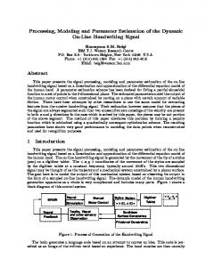
for each school. This cost function was discussed above. Since this process requires an initial guess, we used the values from the previous step; that is, we choose the vector p(w) for the w found in step (b) above. d. Refining the parameter ranges We now have a wetness parameter w for each school (step (b)) and a set of “best parameters” p for each school (step (c)). For each parameter pn consider the set of 32 points in the plane which consists of (w, pn) for each of the 32 campuses obtained from steps (b) and (c) above. Since our parameterization in terms of wetness is that each parameter is a linear function of wetness, we may fit a straight line to the 32


Ackleh et al.

Page 7

school data, for each of the 14 parameters. The linear regression in Figure 2 illustrates the procedure.


Once this line is found, we refine the initial parameter ranges found in step (a) by using the value of the linear regression line at w = 0 for the “dry” value and the value of the line at w = 1 for the “wet” value. We set these values to pnwet and pndry. These values form a new interval for the parameter. e.

Repeat steps (b)–(d) until convergence and compute standard deviation for w By repeating steps (b)–(d) we can refine the ranges of the parameters, i.e., we can obtain iterates of pnwet and pndry until these iterations converge. Once convergence occurs and we have the final estimates for wetness w for each school, we can compute the standard deviation for w at each school. This can be done using similar ideas from standard regression formulations in statistics [10,12,15,18]. To obtain this analysis, we need to compute the sensitivity vector


(3.1)

where T in (3.1) denotes the transpose of a vector. Since we cannot compute , i = l, …, l + 4, directly from our model, we use the following forward difference approximation:

h is taken to a small positive constant. With these approximations we can compute the following approximation of:


Under the assumptions of classical nonlinear regression theory, we know that if ε̂i = (0, σ2), where ε̂i is the difference between the observation and the model at time ti, then the least squares estimate w* is expected to be asymptotically normally distributed. In particular, for large samples we may assume

where w0 is the true minimizer and σ2{XT(w0)X(w0)}−1 is the true covariance matrix (see, e.g., [10,12,15,18]. Since we do not have w0 and σ2, we follow a standard


Ackleh et al.

Page 8

statistical practice [2,6,18]: substitute the computed estimate w* for w0 and approximate σ2 by


Then we take

to be the standard deviation for the parameter.

4 Parameter Estimation Results We begin with the initial ranges given in Table 2 and iterate using the above parameter estimation algorithm 15 times. In Table 2 we provide the resulting estimates of pnwet and pndry for the 5th and 15th iterations. In Figure 3 we present plots for the dry and wet values (i.e., pndry and pnwet for all the 15 iterations.


We now fix the parameter values in Table 2 and Figure 3 in our model and find the best wetness w that fits the model to each of the 32 campus data set (step (b)). The estimated wetness value w, the standard deviation for the wetness and the model residual error for the fifteenth iteration are given in Table 3. In Figure 4 we present plots of the wetness which result from each iteration. Notice that the estimated wetness for School 17 is on the high end of the wetness spectrum (w = 0.55) and that for School 13 is on the low end (w = 0.01), which agrees with the fact that indeed the environment for School 17 is wet and that for School 13 is dry. According to Wechsler et al. [30], Dowdall and Wechsler [14], Hingson and Howland [17] there is a positive correlation between the wetness of an environment and the level of drinking. Thus, if one accepts this theory then the results in Table 3 are useful in the sense that they provide a measurement/scale (the value of the wetness w) of the drinking activity/level on a particular campus.


In Figures 5–8, we present the data (o’s), the data plus and minus the standard deviation (+’s) and the model output (solid lines) for four campuses. In order to give the reader an idea of the range and variety in the quality of the fits for the 32 campuses, in these four figures we present the model-to-data fit for a dry campus, for a wet campus, for a campus with the lowest residual error and for a campus with highest residual error. We point out, however, that all the 32 fits were quite satisfactory, with the model output within two standard deviations of the data. In Figure 5 the fit for School 13 (dry environment) is presented and in Figure 6 the fit for School 17 (wet environment) is shown. In Figures 7 and 8 we present the model-to-data fits for School 23 (lowest residual error) and for School 5 (highest residual error), respectively. Note that even School 5, which had the highest residual error, enjoys a satisfactory model to data fit. In order to connect this model with externally collected data, we compare our inferential wetness index with alcohol outlet density, a quantity of interest to public health scientists. Outlet density, the number per square mile of establishments that sell alcohol, is a measure of physical availability of alcohol. In Figure 9 we show the correlation between wetness and outlet density for the 32 campuses in the study. The R2 of 0.2293 is interpreted to mean that 23% of the variance in wetness appear to be explained by variance in outlet density.


Ackleh et al.

Page 9


One of the many school attributes that contribute to differences in drinking behavior is the residential nature of the campus. Commuter schools, where students typically spend less time on campus and tend to drink less, are often treated differently in terms of policy and analysis. Toward that end, we have removed commuter campuses from this outlet density comparison, and in Figure 10 we see a modest increase in correlation, with an R2 of 0.3112.

5 Applications of Policy Intervention In this section, we use the parameter estimates obtained in Section 4 to explore the effects of two hypothetical interventions policies on the student distribution of a particular campus. 5.1 A policy for reducing wetness


If a university were concerned about the drinking status of the students on its campus, wetness is one of the few variables that may be controlled by the local government. To understand the model’s response to such an intervention policy, we focus on a campus that is known to have a wet environment, School 17. We use the values of pnwet and pndry from the fifteenth iteration given in Table 2. We run a model simulation for 10 years with the wetness parameter w = 0.53, obtained from Table 3. We then run three more simulations, again for 10 years, except that we begin the simulations with w = 0.53 and then reduce w by 20%, 40%, and 60% at the start of the fifth year. We then calculate the ratio of the average student population resulting from the wetness reduction and the original simulation. Since the model invariably reaches equilibrium by the 5th or 6th year, we took the average of the final year of the simulation. These ratios are given in Table 4. This table gives the percent change in the average student population resulting from a percent change in the wetness parameter. For example, one can see that a 20% decrease in wetness results in a 19% increase in abstainers and 7% decrease in bingers, while a 60% decrease in wetness results in approximately 100% increase in abstainers and 27% decrease in bingers. A clear pattern from Table 4 is that the model predicts that a decrease in wetness will result in more abstainers and light drinkers and fewer moderate, problem, and binge drinkers. Also, it seems that the effect is nearly linear, i.e., doubling the percent decrease in wetness approximately doubles the effect on the student population. Figure 11 gives the plots resulting from the 60% wetness reduction. Notice that although we show a 10-year simulation, the effect of wetness reduction on the student population is almost immediate.


Since School 17 is on the higher end in terms of wetness, we want to test if the same results occurred at a more moderately wet campus. So we repeated the exact same calculations as above for School 21, which has a wetness of w = 0.32 (Table 3). In Table 5 we present the resulting ratios for student averages. As in the case for School 17, the model predicts that wetness reduction is an effective way of controlling drinking on a college campus. In Figure 12 we present the plots resulting from the 60% wetness reduction. 5.2 Penalizing students who drink heavily We now consider the effect of penalizing students who drink heavily. In practice, this may involve putting a student on academic probation, or in extreme cases, expelling the student from the university if this student is caught drinking several times. Adoption of this type of intervention may be more feasible for administrators at private universities than at some public institutions. We assume that enforcing such a policy will affect the student population in two ways. First, this will increase the dropout rates of bingers, problem drinkers, and possibly moderate drinkers (those who are caught several times and expelled). Second, once the university develops a reputation as non-drinker friendly, there may be the after effect that fewer students who partake Math Comput Model. Author manuscript; available in PMC 2010 August 1.

Ackleh et al.

Page 10

in drinking apply to enrollment, hence reducing the recruitment rates (cj’s) for bingers and problem drinkers.


For a fair comparison, we again use data from School 17 to test the effect of such a policy (in comparison with reducing wetness policy) on the distribution of the student population. As previously mentioned, we assume that the effect of penalizing drinkers is two-fold, resulting initially in increased dropout rates for moderate, problem and binge drinkers, and later in lower recruitment rates for those same compartments. Recall also that since , a decrease in the recruitment rates of problem, binge and moderate drinkers implies an increase in the recruitment rates for abstainers and light drinkers. We consider two scenarios, where the second one is simply a more severe version of the first one. In scenario 1, we assume that penalizing students who drink will cause a 25% increase in the dropout rates for problem and binge drinkers and a 15% increase in the dropout rate for moderate drinkers. We assume that this policy is enforced at the beginning of the 5th year of a 12-year simulation. Following this action by the university, we assume that the incoming student population reacts and that the incoming rates for problem and binge drinkers decrease by 25% and the incoming rate for moderate drinkers decreases by 15%. We then evenly distribute these drops into the abstainer and light drinker compartments to ensure that


. We assume that this reaction by the incoming students takes place at the beginning of the 9th year. In scenario 2, we repeat the assumptions from scenario 1 except in this case we increase the dropout rates for problem and binge drinkers by 50% and increase the dropout rate for moderate drinkers by 25%. Further, we decrease the incoming rates for bingers and problem drinkers by 50% and decrease the incoming rate for moderate drinkers by 25%. The ratios of the population averages for these two scenarios are presented in Table 6. In Figure 13 we plot the student population resulting from the second scenario. We can see that our model predicts that it is much more effective to reduce wetness than to leave wetness unaffected and penalize drinking students on a wet campus. We now repeat the same calculations of the penalization intervention for School 21. Table 7 provides the ratios for the yearly student averages in each of the five drinking compartments. Notice that in this case, as in the School 17 case, such an intervention policy seems to be relatively ineffective in comparison with a reduction in wetness policy. Figure 14 shows the results of Scenario 2 for this campus.


6 Conclusions While developing a mathematical model to describe a particular phenomenon can prove to be a challenging task, trying to use the model to make predictions that are comparable to real data can prove to be technically very difficult. As previously mentioned, for relatively small-scale problems like this one, traditional parameter estimation techniques can prove impractical. While the method developed here is not a conventional method, the estimates obtained and the model-to-data fits presented are very satisfactory (especially when considering the fact that we have provided fits for 32 campuses). The obvious value of this is that once the model has now been validated with data, it can be used to make predictions. These predictions would be valuable to policy makers or to university administrators who are concerned about the state of drinking among the student population. To understand the effect of intervention polices on reducing the number of binge drinkers on campus we tested two hypothetical policies: 1) reduction of wetness, and 2) penalizing students Math Comput Model. Author manuscript; available in PMC 2010 August 1.

Ackleh et al.

Page 11


who are caught drinking on campus. Our numerical results indicate that reducing wetness is a much more effective policy in controlling the fraction of bingers, problem drinker and even moderate drinkers. In fact, reducing wetness by 60% results in a predicted 27% reduction of bingers at School 17 (Table 4). In contrast, increasing the dropout rate of bingers (due to expulsion from campus) by 50% and reducing their recruitment rates by 50% result in only 2% fewer bingers on campus (Table 6).

References

NIH-PA Author Manuscript NIH-PA Author Manuscript

1. Ackleh AS. Parameter estimation in a structured algal coagulation-fragmentation model. Nonlinear Anal 1997;28:837–854. 2. Ackleh AS, Banks HT, Deng K, Hu S. Parameter Estimation in a Coupled System of Nonlinear SizeStructured Populations. Math Biosci Eng 2005;2:289–315. 3. Ackleh AS, Fitzpatrick BG, Hallam T. Approximation and parameter estimation problems for algal aggregation models. Math Models Methods Appl Sci 1994;4:291–311. 4. Ackleh AS, Fitzpatrick BG. Estimation of discontinuous parameters in general nonautonomous parabolic systems. New directions in control and automation, I (Limassol, 1995), Kybernetika 1996a; 32:543–556. 5. Ackleh AS, Fitzpatrick BG. Estimation of time dependent parameters in general parabolic evolution systems. J Math Anal Appl 1996b;203:464–480. 6. Adams B, Banks HT, Banks JE, Stark JD. Population Dynamics Models in Plant-Insect HerbivorePesticide Interactions. Math Biosci 2005;196:39–64. [PubMed: 15982675] 7. Baer JS, Kivlahan DR, Marlatt GA. High-risk drinking across the transition from high school to college. Alcohol Clin Exp Res 1995;19:54–61. [PubMed: 7771663] 8. Banks HT, Fitzpatrick BG. Statistical methods for model comparison in parameter estimation problems for distributed systems. J Math Biol 1990;28:501–527. 9. Banks, HT.; Kunisch, K. Estimation Techniques for Distributed Parameter Systems. Birkhuser; Boston: 1989. 10. Bates, DM.; Watts, DG. Nonlinear Regression Analysis and Its Applications. Wiley Series in Probability and Statistics; New York: 1988. 11. Congress of the U.S. Under the Influence: The Binge Drinking Epidemic on College Campuses, in Senate Committee on Governmental Affairs. US Government Printing Office; Washington D.C: 2002. 12. Davidian, M.; Giltinan, DM. Nonlinear Models for Repeated Measurement Data. Chapman and Hall/ CRC; New York: 1995. 13. DeJong W, Schneider SK, Towvim LG, Murphy MJ, Doerr EE, Simonsen NR, Mason KE, Scribner RA. A multisite randomized trial of social norms marketing campaigns to reduce college student drinking. J Stud Alcohol 2006;67:868–879. [PubMed: 17061004] 14. Dowdall GW, Wechsler H. Studying college alcohol use: widening the lens, sharpening the focus. J Stud Alcohol 2002;14(Suppl):14–22. 15. Gallant, AR. Nonlinear Statistical Models. Wiley Series in Probability and Statistics; New York: 1987. 16. Hingson R, Heeren T, Winter M, Wechsler H. Magnitude of alcohol-related mortality and morbidity among U.S. college students ages 18–24: changes from 1998 to 2001. Annual review of public health 2005;26:259–279. 17. Hingson RW, Howland J. Comprehensive community interventions to promote health: implications for college-age drinking problems. J Stud Alcohol Suppl 2002;14:226–240. [PubMed: 12022727] 18. Huet, S.; Bouvier, A.; Poursat, M.; Jolivet, E. Statistical Tools for Nonlinear Regression: A Practical Guide with S-PLUS and R Examples (Springer Series in Statistics). New York, NY: 2003. 19. Integrated Postsecondary Education Data System. National Center for Education Statistics, Institute of Education Sciences, U.S. Department of Education. 2007. http://nces.ed.gov/ipedspas


Ackleh et al.

Page 12


20. McCabe SE, Schulenberg JE, Johnston LD, O’Malley PM, Bachman JG, Kloska DD. Selection and socialization effects of fraternities and sororities on US college student substance use: a multi-cohort national longitudinal study. Addiction 2005;100:512–524. [PubMed: 15784066] 21. NIAAA. A Call to Action: Changing the Culture of Drinking at US Colleges. US: DHHS; 2002. 22. Perkins HW, Haines MP, Rice R. Misperceiving the college drinking norm and related problems: a nationwide study of exposure to prevention information, perceived norms and student alcohol misuse. J Stud Alcohol 2005;66:470–478. [PubMed: 16240554] 23. Perkins HW, Meilman PW, Leichliter JS, Cashin JR, Presley CA. Misperceptions of the norms for the frequency of alcohol and other drug use on college campuses. J Am Coll Health 1999;47:253– 258. [PubMed: 10368559] 24. Reis J, Riley WL. Predictors of college students’ alcohol consumption: implications for student education. J Genet Psychol 2000;161:282–291. [PubMed: 10971907] 25. Schulenberg JE, Maggs JL. A developmental perspective on alcohol use and heavy drinking during adolescence and the transition to young adulthood. J Stud Alcohol Suppl 2002;14:54–70. [PubMed: 12022730] 26. Scribner R, Ackleh AS, Fitzpatrick BG, Jacquez G, Thibodeaux J, Rommel R, Simonsen N. Ecosystems modeling of college drinking-development of a compartmental model. 2007 In revision. 27. Scribner R, Mason K, Theall K, Simonsen N, Schneider SK, Towvim LG, DeJong W. The contextual role of alcohol outlet density in college drinking. J Stud Alcohol Drugs 2008;69:112–20. [PubMed: 18080071] 28. Thombs DL, Wolcott BJ, Farkash LG. Social context, perceived norms and drinking behavior in young people. J Subst Abuse 1997;9:257–267. [PubMed: 9494953] 29. Wechsler H, Dowdall GW, Davenport A, Castillo S. Correlates of college student binge drinking. Am J Public Health 1995;85:921–926. [PubMed: 7604914] 30. Wechsler H, Kelley K, Weitzman ER, SanGiovanni JP, Seibring M. What colleges are doing about student binge drinking. A survey of college administrators. J Am Coll Health 2000;48:219–226. [PubMed: 10778022] 31. Wechsler H, Lee JE, Gledhill-Hoyt J, Nelson TF. Alcohol use and problems at colleges banning alcohol: results of a national survey. Journal of Studies on Alcohol 2001;62:133–141. [PubMed: 11327179] 32. Wechsler H, Lee JE, Nelson TF, Lee H. Drinking and driving among college students: the influence of alcohol-control policies. American Journal of Preventive Medicine 2003;25:212–218. [PubMed: 14507527] 33. Weitzman ER, Nelson TF, Lee H, Wechsler H. Reducing drinking and related harms in college: evaluation of the “A Matter of Degree” program. American Journal of Preventive Medicine 2004 2004;27:187–196.

NIH-PA Author Manuscript Math Comput Model. Author manuscript; available in PMC 2010 August 1.

Ackleh et al.

Page 13

NIH-PA Author Manuscript Figure 1.


Five compartment model of college drinking. All transfers are shown. Here N1, N2, N3, N4, and N5 are the numbers of abstainers, light drinkers, moderate drinkers, problem drinkers, and binge drinkers, at time t, respectively. Double arrows indicate that the movement may be in

either direction. Also, and student population, respectively.

are fractions of bingers and drinkers in the


Ackleh et al.

Page 14


Figure 2.

Linear regression of w versus s53.


Ackleh et al.

Page 15

NIH-PA Author Manuscript NIH-PA Author Manuscript NIH-PA Author Manuscript

Figure 3.

Plots of pndry and pnwet for each iteration.


Ackleh et al.

Page 16


Figure 4.

Plots of wetness w for each iteration and for each school.


Ackleh et al.

Page 17


Figure 5.

Least squares fit for School 13 (Low wetness).


Ackleh et al.

Page 18


Figure 6.

Least squares fit for School 17 (High wetness).


Ackleh et al.

Page 19


Figure 7.

Least squares fit for School 23.


Ackleh et al.

Page 20


Figure 8.

Least squares fit for School 5.


Ackleh et al.

Page 21


Figure 9.

Outlet density vs. wetness for the 32 surveyed campuses.


Ackleh et al.

Page 22


Figure 10.

Outlet density vs. wetness for the 20 surveyed residential campuses.


Ackleh et al.

Page 23

NIH-PA Author Manuscript NIH-PA Author Manuscript Figure 11.

Results of wetness intervention policy for School 17. Wetness is reduced from w = 0.53 initially to w = 0.212 after 4 years.


Ackleh et al.

Page 24


Figure 12.

Results of wetness intervention policy for School 21. Wetness is reduced from w = 0.32 initially to w = 0.128 after 4 years.


Ackleh et al.

Page 25


Figure 13.

Results of penalizing students intervention policy for School 17. Dropout rates for problem and binge drinkers are increased by 50% percent and those for moderate are increased by 25%. While recruitment rates for problem and binge drinkers are decreased by 50% and for moderate drinkers are decreased by 25% (scenario 2).


Ackleh et al.

Page 26


Figure 14.

Results of penalizing students intervention policy for School 21. Dropout rates for problem and binge drinkers are increased by 50% percent and those for moderate are increased by 25%. While recruitment rates for problem and binge drinkers are decreased by 50% and for moderate drinkers are decreased by 25% (scenario 2).



19

Year 3

19

21

Year 2

Year 4

18

Abstainers

Year 1

School 17

45

59

46

30

Light Drinkers

69

66

56

51

Moderate Drinkers

39

30

46

36

Problem Drinkers


Survey data for School 17.

82

84

71

61

Bingers


Table 1 Ackleh et al. Page 27



NIH-PA Author Manuscript 18.2750 4.1022 5.1381 4.4721 0.8180 3.8805 2.6873 0.1605 0.5278 3.0677 0.5716 0.1227 1.3029

s52

s53

r41

r24

r25

r52

r34

r35

r53

r54

r21

n12

0.6490

s12

s32

p dry

parameter

initial guess

13.7727

1.4426

0.5611

2.2498

3.2995

0.6451

2.1707

11.2545

2.4334

4.8225

3.4184

2.5082

4.1036

36.7129

p wet

Initial guess, fifth iteration and fifteenth iteration for pnwet and pndry.

1.3322

0.6803

0.6435

3.0716

0.3366

0.2221

2.8132

3.2903

0.7732

4.7461

5.1737

4.1341

18.2077

0.5743

p dry

fifth iteration

13.1932

0.7136

0.6294

2.3946

4.0130

0.5490

1.7322

12.9601

2.2009

4.3660

3.3074

2.3715

4.2492

36.7323

p wet

1.0797

1.1437

0.7805

3.0570

0.2063

0.1995

2.6689

2.4489

0.7080

4.9143

5.2351

4.1193

18.0406

0.3578

p dry

fifteenth iteration


Table 2

13.6048

0.0844

0.8731

2.8923

4.7326

0.7489

2.0387

15.1165

1.6779

4.1797

3.1509

2.3537

4.6436

37.1426

p wet

Ackleh et al. Page 28


Ackleh et al.

Page 29

Table 3

Wetness, standard deviation for wetness and model residual error for each campus


wetness

standard deviation for wetness

least squares error

School 1

0.1900

0.0250

0.0260

School 2

0.2400

0.0356

0.0232

School 3

0.4800

0.0594

0.0213

School 4

0.1300

0.0142

0.0331

School 5

0.1200

0.0133

0.0410

School 6

0.2300

0.0305

0.0233

School 7

0.1100

0.0077

0.0326

School 8

0.3800

0.0454

0.0248

School 9

0.1100

0.0118

0.0404

School 10

0.2100

0.0290

0.0210

School 11

0.3000

0.0460

0.0360

School 12

0.1400

0.0101

0.0323

School 13

0.0900

0.0059

0.0322

School 14

0.1100

0.0308

0.0316

School 15

0.3300

0.0386

0.0212

School 16

0.1400

0.0431

0.0274

School 17

0.5300

0.0623

0.0275

School 18

0.1400

0.0387

0.0382

School 19

0.4800

0.0453

0.0213

School 20

0.2500

0.0309

0.0222

School 21

0.3200

0.0420

0.0259

School 22

0.1200

0.0155

0.0390

School 23

0.3400

0.0328

0.0163

School 24

0.4700

0.0549

0.0254

School 25

0.2700

0.0353

0.0344

School 26

0.4000

0.0675

0.0279

School 27

0.3500

0.0373

0.0264

School 28

0.3300

0.0449

0.0294

School 29

0.1300

0.0097

0.0277

School 30

0.1900

0.0168

0.0384

School 31

0.3300

0.0373

0.0249

School 32

0.3600

0.0336

0.0214



NIH-PA Author Manuscript 1.4868 2.0304

60%

1.1868

20% 40%

abstainers

reduction in wetness

1.6683

1.4321

1.1970

light

0.6015

0.7651

0.9042

moderate

Wetness reduction and compartmental distribution changes

Ratios of the original student population versus the student population after a wetness reduction.

0.8342

0.9084

0.9586

problem

0.7306

0.8437

0.9283

heavy episodic





NIH-PA Author Manuscript 1.4545 1.9105

60%

1.1807

20% 40%

abstainers

reduction in wetness

1.2252

1.1836

1.0983

light

0.6145

0.7437

0.8747

moderate

School 21:Wetness reduction and compartmental distribution changes

Ratios of the original student population versus the student population after a wetness reduction.

0.7979

0.8898

0.9530

problem

0.7043

0.8265

0.9222

heavy episodic






Scenario 2

Scenario 1

Scenario

0.9533

0.9959

abstainers

1.1205

1.1162

light

0.9331

0.9180

moderate

School 17:Dropout/matriculation rates and compartmental distribution changes

1.0226

1.0124

problem

Ratios of the original student population versus the student population after a policy of penalizing drinking students is enforced

0.9798

0.9878

heavy episodic






Scenario 2

Scenario 1

Scenario

0.9012

0.9496

abstainers

1.1138

1.0916

light

0.8783

0.8867

moderate

School 21:Dropout/matriculation rates and compartmental distribution changes

1.0459

1.0258

problem

Ratios of the original student population versus the student population after a policy of penalizing drinking students is enforced.

0.9898

0.9935

heavy episodic




Ecosystem Modeling of College Drinking: Parameter Estimation and ...

Ecosystem Modeling of College Drinking: Parameter Estimation and ...

Suggest Documents

Modeling, parameter estimation, and open-loop

Exam scheduling: Mathematical modeling and parameter estimation

Processing, Modeling and Parameter Estimation of ... - Semantic Scholar

Dynamic Modeling and Parameter Estimation of a Cu ...

Modeling and parameter estimation of the SOS ...

Modeling and parameter estimation of rheological objects for ...

Providing a New Approach for Modeling and Parameter Estimation of

Rapid Modeling and Parameter Estimation of Partial ... - MDPI

Parameter estimation for basin-scale ecosystem ... - Semantic Scholar

Parameter Estimation in Biomass Crop Models - Agro-ecosystem

Parameter optimization and analysis of ecosystem ... - IngentaConnect

Parameter Estimation of Electromechanical

Dynamic Modeling, Parameter Estimation, and Uncertainty ...www.researchgate.net › publication › fulltext › Dynamic-

Vehicle Modeling and Parameter Estimation Using Adaptive ... - DCSL

Modeling and parameter estimation for point-actuated ... - bu people

Application of a Parameter-Estimation Technique to Modeling the ...

BAYESIAN ESTIMATION OF RANDOM PARAMETER

PARAMETER ESTIMATION OF A NONLINEAR

PARAMETER ESTIMATION OF A NONLINEAR

DISTRIBUTED LINEAR PARAMETER ESTIMATION ...

CosmoHammer: Cosmological parameter estimation

Parameter Estimation Through Ignorance

Robust parameter estimation

Model Parameter Estimation