ABSTRACT. Constructed wetlands are complex dynamic ecosystems. Ecosystem-level modeling of the processes that take place in a constructed wetland is a ...
C. Laspidou & V. Vaina, Int. J. of Design & Nature and Ecodynamics. Vol. 3, No. 4 (2009) 273–280
ECOSYSTEM MODELING OF SEDIMENT DYNAMICS IN THE CONSTRUCTED WETLAND CARLA IN CENTRAL GREECE C. LASPIDOU1 & V. VAINA2 and Environmental Engineering Laboratory, Department of Civil Engineering, University of Thessaly, Pedion Areos, Greece EYATH--Thessaloniki Water Supply and Sewerage Co. S.A., Egnatia 127, Thessaloniki, Greece.
1Hydromechanics
ABSTRACT Constructed wetlands are complex dynamic ecosystems. Ecosystem-level modeling of the processes that take place in a constructed wetland is a useful tool for understanding wetland function and structure and for making predictions. We present a primary productivity model for the wetland that is currently under construction in the area of Carla in central Greece, restoring one of the most important wetlands in Europe that was drained in 1962. The model includes the area’s hydrology and geomorphology and is used to explore the role of different wetland structures and functions on the dynamics of primary producers and sediments in the constructed ecosystem, in order to provide a better understanding of the processes involved and the nutrient dynamics in these processes. Keywords: constructed wetland, ecosystems modeling, primary productivity modeling, sediment dynamics.
1 INTRODUCTION Wetlands are lands transitional between terrestrial and aquatic systems where the water table is usually at or near the surface, or the land is covered by shallow water [1]. They store water that can be used for irrigation or for other uses, while they protect from flooding the crops and the inhabited areas downstream. Wetlands are invaluable ecosystems because of the many beneficial properties they have. They regulate the climate of the greater area surrounding it, limiting extreme weather phenomena. The water, plants and soil in wetlands retain carbon dioxide from the atmosphere, thus helping reduce the greenhouse effect. Other than their productive and ecological importance, wetlands are a beautiful natural environment and the habitat of a large variety of animal and plant species. Wetlands naturally clean the water that flows through them; Mitsch and Gosselink [2] call wetlands the “kidneys” of the earth, as they retain phosphorus, nitrogen and heavy metals from the water as well as pesticides, insecticides and other toxic substances. Since they can be sinks for almost any chemical, applications of constructed treatment wetlands are quite varied, with thousands of applications worldwide treating domestic wastewater, mine drainage, nonpoint source pollution, stormwater runoff, landfill leachate and livestock operations [3]. The design of treatment wetlands requires particular attention to hydrology, chemical loading, soil physics and chemistry, and wetland vegetation [4]. Nutrient removal by wetlands is attributed to shallow low-velocity water that allows maximum nutrient absorption and settling, high primary productivity that leads to high nutrient uptake, a combination of aerobic and anaerobic conditions that facilitate chemical transformations, and peat accumulation that permanently buries chemicals. Mathematical and simulation modeling in combination with field and experimental data provides a powerful method of evaluating the complex processes operating in such systems, in which we see the interactions of physical, chemical, macrobiological and microbiological processes that create a highly complex set of behaviors [5]. We develop a sophisticated ecosystem model of the constructed Carla wetland in Thessaly, Greece focusing initially on primary productivity dynamics and then extending the model to include sediment dynamics, thus ultimately predicting sediment retention by the wetland under different hydrologic conditions. © 2009 WIT Press, www.witpress.com ISSN: 1755-7437 (paper format), ISSN: 1755-7445 (online), http://journals.witpress.com DOI: 10.2495/D&NE-V3-N4-273-280
274
C. Laspidou & V. Vaina, Int. J. of Design & Nature and Ecodynamics. Vol. 3, No. 4 (2009)
2 MATERIALS AND METHODS Most wetland models have been only applicable to the site for which they are developed. Wang and Mitsch [6] built a wetland ecosystem model and had the opportunity to test it on four different wetlands at the Des Plaines River Wetland Demonstration Project site in the US, each of which had different hydrologic conditions. Such a model could then be used to give detailed predictions of the capabilities of constructed wetlands to retain nutrients and sediments, since it is generalized to fit more than one wetland. We develop an ecosystem-level model based on that by Wang and Mitsch [6] and adapt it to the conditions relevant to the hydrology and geomorphology of the Carla wetland. 2.1 Site description – Hydrology The reservoir is located approximately 20 km northwest of the city of Volos in the prefecture of Magnesia in central Greece. The elevation-surface-storage curves for the reservoir were obtained from the technical study of the Karla reservoir and associated works [7]. Minimum water levels are set at 45.35 m above sea level (a.s.l.) with a water surface area of 27.83 km2 and a dead volume of 20.24 × 10⁶ m3 [7]. Taking into account that the lowest elevation at the bottom of the reservoir is about 43.5 m a.s.l., the maximum lake depth at the end of the dry season will be about 1.85 m. Water will be pumped in from the river Pineos (Qriver) through a pumping station with a capacity of 14 m3/s, and will be pumped out to cover irrigation needs of the area. Maximum water level available for irrigation is 48.8 m a.s.l., with a useful storage water available for irrigation of 128.05 × 10⁶ m3. Maximum flood water level is at 50 m a.s.l., which corresponds to a storage of 195.16 × 10⁶ m3. Once the maximum flood water level is reached, water is allowed to flow out of the wetland via a tunnel that discharges water into the adjacent gulf of Pagasitikos (QPagas) at a rate of 8.5 m3/s [8]. This way, flooding events are limited. This information is incorporated (with a series of IF-THEN statements) in the development of a hydrologic mass balance for the reservoir. Additional inflows into the reservoir are precipitation (Qpcptn), inflow from the watershed (Qw/shed) and inflow from the surrounding irrigated area drainage tiles (Qdrain). Outflows include QPagas whenever it is deemed necessary, losses to the underlying aquifer (Qaquifer), water pumped out of the reservoir for irrigation (Qirrig), as well as losses due to evapotranspiration (QET). Therefore, we can define the following reservoir water volume (V) mass balance.
dV = Qriver + Qpcptn + Qw/shed + Qdrain − Qaquifer − Qirrig − QPagas − QET dt
(1)
Equation (1) provides us with a way to calculate the change in the volume of the Carla reservoir as a function of time (dV/dt, in m3/week). All other quantities in eqn. (1) were obtained from the Environmental Impact Assessment (EIA) study for the Carla reservoir. These values for a typical year are shown in Table 1. To calculate the wetland surface area (Aw, in m2) corresponding to the volume calculated by eqn. (1), we take into account the reservoir geometry. This is done with the elevation-surface-storage curves; thus, we use the mass balance in eqn. (1) to calculate the reservoir volume at different times, and the elevation-surface-storage curves to calculate the corresponding surface area. The average depth of the water in the wetland (DW) is then found by dividing the calculated storage volume by the corresponding reservoir surface. 2.2 Simulation methods Projections of field data were obtained from the EIA for the Carla reservoir and from the Environmental Report prepared by the Greek Ministry of Environment Regional Planning and Public Works [9]. Three
C. Laspidou & V. Vaina, Int. J. of Design & Nature and Ecodynamics. Vol. 3, No. 4 (2009)
275
Table 1: Inflows/outflows of the Carla reservoir for a typical year and initial values of state variables for the Carla wetland reservoir. Inflows/outflows
Initial values of state variables
Qriver = 148.2 × 10⁶ m3 Qpcptn = 42.41 × 10⁶ m3 Qw/shed = 96.86 × 10⁶ m3 Qdrain = 6.73 × 10⁶ m3 Qaquifer = 130.8 × 10⁶ m3 Qirrigation = 107.6 × 10⁶ m3 QET = 37.80 × 10⁶ m3
V = 115.3 × 10⁶ m3 [7] PLAN = 6.0 × 10⁶ m3 [6] PERI = 2.0 × 10⁶ m3 [6] MAC = 2.0 × 10⁷ m3 [6]
submodels were developed, including one for hydrology, one for primary productivity and one for sediments. A set of nonlinear, ordinary differential equations was used to describe the submodels. The model was integrated by using the software STELLA™ VIII, a high level visual-oriented programming and simulation language [10]. Fourth-order Runge–Kutta was used as the integration method with a time step of 0.1 week. Initial values for all quantities were taken either from the above reports, or were estimated from relevant values reported in the literature, taking into account the storage volume and surface area of the reported wetland and that of Carla, and sizing them accordingly (shown in Table 1). 2.3 Primary productivity modeling Primary production is the amount of carbon fixed by plants per unit area over time via photosynthesis [2]. In a wetland, primary producers are planktonic diatoms or phytoplankton (PLAN, in g), macrophytes or rooted aquatic plants (MAC, in g) and periphyton (PERI, in g) [2]; thus, the primary productivity model includes these three variables. Similar to eqn. (1), we develop mass balances for each one of these state variables. Phytoplankton dynamics are described in a manner similar to Wang and Mitsch [6] by the following simplified processes: growth, respiration, settling and exportation with outflow (eqn. 2). d PLAN = SolRad ⋅ SE PLAN ⋅ a 1 ⋅ AW ⋅ q G − PLAN ⋅ rPLAN ⋅ q G ����� ������� � ������� dt PHYTOPLANKTON GROWTH, in g/week
PHYTOPL. RESPIRATION, in g/week
(2)
− PLAN ⋅ vsett DW ⋅ q S − PLAN ⋅ QOUT �������� � �� ���� � PHYTOPLANKTON SETTLING, in g/week
PHYTOPLANKTON OUTFLOW, in g/week
Phytoplankton growth rate is directly related to solar radiation (SolRad, in kcal/m2 week), phytoplankton solar efficiency (SEPLAN, a number ranging from 0 to 1), the surface area of the wetland and a temperature function that expresses growth and respiration dependence on water temperature −2.3⋅ (TW − 25) / (Tw in °C) (q G = e . The temperature function was assumed to follow a symmetrical temperature optimum curve described by Jorgensen et al. [11], with an optimal temperature for biological activity set to 25°C. The constant a1 is the inverse of the energy per biomass ratio and converts the kcal of solar radiation into g of biomass (a1 = 0.2439 g/kcal as in Wang and Mitsch [6]). Phytoplankton respiration rate is proportional to the corresponding respiration rate (rPLAN/week)
276
C. Laspidou & V. Vaina, Int. J. of Design & Nature and Ecodynamics. Vol. 3, No. 4 (2009)
and has the same temperature dependence [1], while phytoplankton settling depends on a settling T − 20 velocity (vsett, 4 m/week [6]) and also has a temperature dependence (q S = 1.024 W ) . The outflow of phytoplankton occurs only with irrigation and exportation to the Pagasitikos gulf, so QOUT = Qirrig + QPagas. Solar radiation data in the area were obtained by measurements of the water temperature of Penios river water, which are presented in the Environmental Report on the reconstruction of Carla by the Ministry of Public Works in Greece [9]. Primary production of macrophytes is a major input of biomass and hence organic matter (OM) to wetland ecosystems. Researchers show a great variety of macrophyte production among wetlands, which suggests that local conditions such as soils, seeding and hydrologic conditions play a major role in the initial growth of macrophytes at the beginning of the growing season. Wang and Mitsch [6] estimated initial coverage by macrophytes at the beginning of the growing season by aerial photographs of four constructed wetlands. We used a similar initial value, adjusted for the surface of the Carla wetland, as it compares to the wetland in the Wang and Mitsch study [6]. In a manner similar to phytoplankton, the macrophyte mass balance was obtained by including growth, respiration and death (eqn. 3). Macrophyte growth was directly proportional to solar radiation and a corresponding efficiency for macrophytes (SEMAC) multiplied by the % coverage of the wetland surface by macrophytes (MACcover) to obtain solar radiation captured. Macrophyte respiration and death was calculated using corresponding rates (rMAC and dMAC, respectively) obtained by Wang and Mitsch [6]. The death rate was input as a function of time and is made to increase from 0 to 1.0 from October to the end of the year, while it was made to gradually drop down to zero by the beginning of spring in March [12]. d MAC = SolRad ⋅ SE MAC ⋅ a 1 ⋅ MACcover ⋅ AW ⋅ q G ������� ��������� � dt
(3)
MACROPHYTE GROWTH, in g/week
−
MAC ⋅ rMAC ⋅ q G �������
MACROPHYTE RESPIRATION, in g/week
− MAC ⋅ d MAC �����
MACROPHYTE DEATH in g/week
Periphyton is different than phytoplankton in that it can only grow attached on macrophytes (either growing or dead), so the extent of its growth depends on the available surface area, and it does not settle but gets lost due to scouring or sloughing from the substratum – modeled by a first-order loss constant SPERI (0.8/week [6]) The surface area for growth (APERI) is estimated by calculating the number of macrophyte stems and finding the stem surface area (assuming that each stem weighs 27 g and has a perimeter of 2.6 cm [6]); thus the area available for periphyton growth is found by the following: APERI = ((MAC + MAC·dMAC)/27)·DW·0.026π. Solar efficiencies for eqns. (2)–(4) were estimated as 0.2%, 2.5% and 0.3%, respectively, based on values found in the literature [6]. d PERI = SolRad ⋅ SE PERI ⋅ a 1 ⋅ APERI ⋅ q G − ������������ � dt PERIPHYTON GROWTH, in g/week
PERI ⋅ rPERI ⋅ q G ������ �
PERIPHYTON RESPIRATION, in g/week
−
PERI ⋅ S PERI �����
(4)
PERIPHYTON SCOURING, in g/week
2.4 Sediment modeling The sediment sub-model has five state variables consisting of standing dead macrophytes (SD), bottom detritus (BD), suspended sediments (SS), active sediments (AS) and deep sediments (DS). The SD mass balance (eqn. 5) includes the plants that die minus the ones that fall in the water; the latter is expressed with a first-order falling rate (rSD,falling, 0.044/ week [6]). d SD = MAC ⋅ d MAC − SD ⋅ rSD,falling dt
(5)
C. Laspidou & V. Vaina, Int. J. of Design & Nature and Ecodynamics. Vol. 3, No. 4 (2009)
277
Bottom detritus includes dead, decaying OM on the bottom of wetlands. Inflows to the mass balance include settling of primary producers, while outflows include decaying of all OM to inert materials and fragmentation of BD to fine particles (eqn. 6): d BD = PHYTsettling + PERIsettling + SDfalling − BD ⋅ rBD,frag − BD ⋅ rBD,decay ⋅ q OM (6) ����� ������� dt BD fragmentation
BD decay
In eqn. 6, rBD,frag and rBD,decay are the rates of fragmentation (0.08/week) and decay (0.006/week) of BD, respectively. The dependence of BD decay on temperature is expressed via the temperature function θOM = 1.047T – 20, where T is the water temperature in °C. Suspended are the sediments in the wetland that are in suspension. They are brought in the wetland with the inflow of Penios river (Qriver), of drainage tiles (Qdrain) and of run–off from the watershed (Qw/shed). We use values for the SS concentrations of the inflows from the literature (SSriver equal to 83.4 g/m3 and SSdrain and SSw/shed equal to 2000 g/m3 [13]). SS outflows include sedimentation to the bottom of the wetland, which occurs with sedimentation velocity vsediment (3 m/week [6]) and outflow out of the wetland with water pumped out for irrigation (Qirrig) and water being discharged to the gulf of Pagasitikos (QPagas). The SS mass balance appears in equation (7). d SS = QPenios ⋅ SSconc,river + (Qrunoff + Qdrainage )⋅ SSconc,runoff ��������� ����������� � dt SS inflow
−
SS ⋅ q sett (Qirrig + QPagas )− SS ⋅ vsediment V WL ��� ����� � ��� ���� SS outflow
(7)
SS sedimentation
Active sediments are defined as the upper layer of the wetland sediments that remain active in the wetland processes and have a constant depth. When additional sediments are deposited on top of that layer, then they are defined as surface. Studies show that the top 2–5 cm of sediments are the most active and are those in which we have changes in nutrients. In this model, we define the top 4 cm as the active layer. The mass balance of AS includes inflows from SS that settle and from BD that gets fragmented; losses are due to the decay of OM in sediments which happens with a rate rAS,decay (5.5 × 10⁻⁵/week [14]) and has a temperature dependence expressed through θOM and due to the final deposition to the DS of all inert matter that remains. d AS 0 = SSsedimentation − BD fragmentation − AS ⋅ rAS,decay ⋅ q OM − AS − AS ��� � ������� AS � dt to Deep Sediments
(8)
AS decay
Finally, the DS represent the final point, the sink of the model. This compartment does not influence the rest of the model, since it is assumed that no decomposition process takes place in this compartment, but a simple deposition of substances that have already been decomposed in other compartments and are completely inert. d DS = ASto DS dt
(9)
3 RESULTS AND DISCUSSION The purpose of ecosystem modeling includes integration of collected data, quantitative description of major pathways or processes through different storage compartments, and presentation of a whole picture at the ecosystem level. One way to achieve this is to draw a system diagram based on
278
C. Laspidou & V. Vaina, Int. J. of Design & Nature and Ecodynamics. Vol. 3, No. 4 (2009)
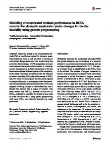
modeling results. A conceptual system diagram of the constructed primary productivity model, where the flows of OM and energy are depicted with Odum energy symbols is shown in Fig. 1. With this diagram, we can see how productive and efficient the wetland is in using solar irradiation and inorganic carbon in the form of CO2 and fixing it to produce OM through the process of photosynthesis. The OM budgets displayed in Fig. 1 were calculated from simulation results using typical hydrology data based on the EIA study for the Carla wetland. Total solar irradiation for the wetland is 113880 kcal/m2 yr, which, using the ratio α1, corresponds to 27776 g dry weight/m2 yr. Out of this quantity, 20 g/m2 yr flow toward the growth of phytoplankton, while 0.8 g/m2 yr are lost by flowing out of the wetland (QOUT), 18.6 g/m2 yr are used up for respiration (shown as dissipated to a “sink”) and 0.6 g/m2 yr settle to the bottom of the wetland. The corresponding quantities for periphyton and macrophytes can be seen in Fig. 1 and follow the same rationale. By calculating the budgets of the flow of energy and OM in this manner, we can calculate that the Carla wetland over a 1 year period shows a solar efficiency (percent of total annual solar radiation converted to gross primary productivity) of 0.61%. This value falls within the range
SS inflow
5391.4
104.8
Suspended sediments in water
5053.7 Solar radiation
Phytoplankton 0, 8
20
18, 6 Periphyton
113880 kcal/m2-yr
0, 6 14
12
26
Active sediments
Macrophytes 125.1
1
61
113179 kcal/m2-yr
67.9 Bottom detritus
64 Dead macrophytes
Carla wetland
23
4.4
4999.1
Deep sediments
Figure 1: Organic matter budgets for the Carla wetland with Odum energy symbols, as calculated from the model for a typical year (all flows in grams of dry weight/m2 yr).
C. Laspidou & V. Vaina, Int. J. of Design & Nature and Ecodynamics. Vol. 3, No. 4 (2009)
279
of values reported by Wang and Mitsch [6] for four constructed wetlands of 0.25–0.93%. It should be emphasized at this point that this value is simply an estimate that includes all the data and assumptions input in the mathematical model and will vary depending on the input data. What we present in this study is a tool, flexible and general enough so that it can accommodate any given data set, yet sophisticated and sensitive to the different processes modeled. Once a more accurate set of data is obtained, the accuracy of the calculated quantities will improve accordingly. In order to compare the autochthonous OM production in the Carla wetland to the allochthonous OM brought in by the river, we first calculate the OM produced by the dead macrophytes and add that to the OM settling that originated from phytoplankton and periphyton, which then becomes BD. The total autochthonous OM is shown in Fig. 1 and equals 78.6 g/m2 yr. Allochthonous OM includes solids that enter the wetland and are not produced in it. These come in from the river, the drainage tiles and the surrounding watershed. Summing up all incoming solids results in the inflow of 5391.4 g/m2 yr, a quantity much higher than that of autochthonous OM production. Thus, 98% of the newly created sediments in the Carla wetland originate from the river and only 2% are created in the wetland. These figures are within the range of reported values for other newly-created wetlands [15]. The value of autochthonous OM production is low and reflects the fact that the wetland is newly created and has relatively low productivity. This is directly related to the fact that the wetland has not had enough time to produce a large quantity of primary producers that are critical in authochthonous OM production. Moreover, inflow of OM is high because we have an influx of high concentrations of sediments in river water, run–off and drainage. In case any construction takes place in the surrounding area, these concentrations are expected to become even higher and to overload the wetland with allochthonous OM. Such high influx of allochthonous sediments influences sediment accumulation in the reservoir, resulting in the deterioration of the wetland, and limiting its beneficial uses. This way, problems are created in irrigation, in the quality and quantity of fish that survive in the wetland and the overall “filling up” of the wetland in a relatively short period of time. The accumulation of sediments in the wetland is estimated by the newly-created sediments during one year of operation of the wetland. All sediments that have been created during 1 year are estimated by adding up AS, DS and BD. This sum is then divided by an average density for sediments (0.6 g/cm3) [15, 16] to find the volume of these sediments. Dividing by the surface of the wetland bottom results in an average accumulation of sediments at the bottom of the wetland. This calculation for the Carla wetland, using the mathematical model and the initial conditions presented here is 12.5 mm per year. This value is within the range of values that are reported in the literature for a newly-created wetland [2]. 4 CONCLUSIONS We developed a detailed ecological model of the processes expected to take place in the Carla wetland which is currently under construction in central Greece. The model consists of three sub-models (one for hydrology, one for primary productivity and one for sediments). The primary producers phytoplankton – periphyton and macrophytes – were included and the hydrologic conditions of the wetland were incorporated in the simulation model. Sediments were modeled in five different forms (SD, BD, as well as active, suspended and DS). Simulation results include a wetland solar efficiency of 0.61%, while an estimate that allochthonous OM importation by the Penios river exceeds the autochthonous OM production. Accumulation of sediments in the wetland was estimated to be 12.5 mm per year. ACKNOWLEDGMENT This research effort is funded by the Greek State Scholarship Foundation (IKY).
280
C. Laspidou & V. Vaina, Int. J. of Design & Nature and Ecodynamics. Vol. 3, No. 4 (2009)
REFERENCES [1] Cowardin, L.M., Carter, V., Golet, F.C. & LaRoe, E.T. Classification of Wetlands and Deepwater Habitats of the United States, FWS/OBS-79/31, U.S. Fish and Wildlife Service: Washington, DC, 103 pp., 1979. [2] Mitsch, W.J. & Gosselink, J.G. Wetlands (3rd ed.), John Wiley & Sons, Inc.: NY, 2000. [3] Laspidou C. Constructed wetlands technology and water quality improvement: Recent advances, Proceedings 9th International Conference on Environmental Science and Technology, 1–3 September 2005, Rhodes Island, Greece, 2005. [4] Gerakis, P.A. & Koutrakis E.T., (eds). Greek Wetlands. Greek Center for Biotopes-Wetlands (EKBY): Athens, 1996 (in Greek). [5] Mitsch, W.J., Horne, A. & Nairn, R.W. (eds.). Nitrogen and phosphorus retention in wetlands. Special Issue of Ecological Engineering, 14, pp. 1–206, 2000. [6] Wang, N. & Mitsch, W.J., A detailed ecosystem model of phosphorus dynamics in created riparian wetlands. Ecological Modeling, 126, pp. 101–130, 2000. [7] Mahairas, A.E., Final Study of the Karla Reservoir and Associated Works, Vol. 1, Technical Review, Greek Ministry of the Environment: Athens, 1995 (in Greek). [8] Moustaka, E. Water Resources Management of the watershed of the under construction lake Carla by use of a Geographic Information System, Thesis, University of Thessaly Publishing: Volos, 2002 (in Greek). [9] Recreation of Lake Carla Environmental-Technical Report, Study of Cost-Benefit and Supporting Studies: Environmental Report – Mathematical Simulation of the Trophic Condition of the Carla Reservoir, Ministry of Public Works, Athens, 1999 (in Greek). [10] Richmond, B. & Peterson, S., STELLA II: Tutorials and Technical Documentation, High Performance Systems: Lyme, NH, 196 p., 1992. [11] Jorgensen, S.E., Mejer, H. & Friis, M., Examination of a lake model. Ecological Modeling, 4, pp. 253–278, 1978. [12] Davis, C.B. & van der Valk, A.G., The composition of standing and fallen litter of Typha glauca and Scirpus fluviatilis. Canadian Journal of Botany, 56, pp. 662–675, 1978. [13] Lazaridou-Dimitriadou, M. Seasonal variation of the water quality of rivers and streams of eastern Mediterranean. Web Ecology, 3, pp. 20–32, 2002. [14] Kadlec, R.H. & Hammer, D.E., Modeling nutrient behavior in wetlands. Ecological Modeling, 40, pp. 37–66, 1988. [15] Fennessy, M.S., Cronk, J.K. & Mitsch, W.J., Macrophyte productivity and community development in created freshwater wetlands under experimental hydrologic conditions. Ecological Engineering, 3, pp. 469–484, 1994. [16] Fennessy, M.S., Brueske, C. & Mitsch, W.J., Sediment deposition patterns in restored freshwater wetlands using sediment traps. Ecological Engineering: the Journal of Ecotechnology, 3, pp. 409-428, 1994.