edge adapted wavelet transform for image compression - eurasip

EDGE ADAPTED WAVELET TRANSFORM FOR IMAGE COMPRESSION Fikri Goksu, Ahmed H.Tewfik Electrical and Computer Engineering Department, University of Minnesota EE/CSci 4-178, 200 Union St SE, 55455, Minneapolis, MN, USA email: {goksu, tewfik}@ ece.umn.edu

ABSTRACT Several approaches have been proposed to improve the compaction performance of the wavelet transform by taking into account the singularities present in the image and their 2D directionalities. This improvement is valid both for compression and de-noising applications. Here, we investigate an edge adaptive wavelet transform which has a better rate-distortion characteristic than the classical wavelet transform. The proposed approach can be viewed roughly as a combination of image segmentation and shape adaptive wavelet transform. The algorithm consists of two steps. In the first step we locate edges by using a sigma filter. In the second step we apply the modified wavelet transform on the separated parts of the image. We provide performance results in terms of rate-distortion curves for both 1D and relatively simple 2D signals. 1. INTRODUCTION The wavelet transform is known for its approximation power. For certain classes of signals the error decay rate can be given as a function of the number of coefficients and the number of vanishing moments that wavelets have. Practitioners have observed that non-negligible wavelet coefficients are locally concentrated around singularities and decay slowly as we move away from singularities. Good performance of wavelets in 1D has made the wavelet transform one of the main tools in signal processing applications, especially denoising and compression. Similar performance was expected for 2D signals but has not been achieved. This is simply because wavelets are better at capturing discontinuities present in 1D signals than they are in 2D signals [1]. This has led researchers to explore enhanced wavelet transforms that are better able to capture singularities present in 2D in a compact manner. In [2], an approximate digital Radon transform is computed in the Fourier domain which maps 1D smooth singularities into points. Then the 1D wavelet transform is used to efficiently represent them. The resulting directional bases are called ridgelets and the transform a ridgelet transform, respectively. They achieve improved performance for objects with straight edges. Ridgelets are combined with multiscale schemes and band pass filtering gives rise to curvelets, [3]. Since non-straight edges become straight locally with increasing scale curvelets achieve better performance for ob-

jects with non-straight edges. These bases are redundant and not applicable for compression but provide nice results for denoising applications. In [4] a local directional representation is developed by combining a multiresolution scheme with directional filter banks which resulted in contourlets. The treatment of edges in these previous two approaches are by aligning the transform bases in the same direction as edges. Another approach is developed in [5] where the edges in the image are decomposed into wedgelets of different orientations. A similar idea is developed in [6]. First singularities are detected vertically and horizontally with foveal wavelets and then these singularities are chained to form edge curves. 1D wavelet transform is applied along the curves to represent them efficiently. Finally, the residual image outside the singularities is represented by a 2D standard wavelet transform efficiently. The main point in these previous two papers is to adaptively represent the singularities efficiently rather than designing directional bases. Both [7] and [8] have approached the problem from a different perspective. The key point is to avoid producing large coefficients from the same edge point in an adaptive manner rather than designing directional bases or removing edges. A Lifting scheme is used to approach the problem which can be decomposed in prediction and update parts. The former introduces prediction operators based on leastsquare fitting while the latter reduces prediction size near edges. Our goal in this paper is also based to detect the singularities in a first step and then apply a modified wavelet transform in the second step. In 1D this corresponds to signal segments separated by individual singular points. Either even length or odd length independent wavelet transforms are performed along these signal segments. The resulting wavelet transform matrix is orthogonal meaning that there is no stability issue involved in the reconstruction. In 2D the picture becomes smooth image regions separated by edge curves and the same idea is applied there. Details to parts of our approach are available in the following sections. Section 2 describes the edge detection process by using the sigma filter. The description of the modified wavelet transform constitutes Section 3. Section 4 shows some performance results in terms of rate-distortion curves. We conclude with some future directions and discussions in Section 5.

2. SMOOTH IMAGE REGION IDENTIFICATION As mentioned above we are using a two step algorithm. The goal of the first step which we describe here is to detect the dominant edge points so that the resulting image will be composed of textures separated by edges. There are many candidate edge detectors available like the simple Prewitt, Sobel or more sophisticated Canny edge detectors to name a few. But they do not exactly fit the purpose that we want to implement. One of the reasons is that all edge detectors when applied to a simple image create many edge points and they may also create edges corresponding to noise. Since the application we intend is compression and we are going to code the edge points in order to be able to reconstruct the signal from the coefficients, we want to detect only dominant edges available in the image. Our Sigma filter [9] models the image as combinations of image regions consisting of constant pixel values corrupted by additive Gaussian noise. For every pixel value a new pixel value is computed iteratively by using neighbouring pixels in a window. The result is a cartoon looking image separated by strong edges. Using a threshold parameter weak edges are wiped out. It is a structure preserving noise removal process. Since we need to find the coordinates of the edges after this process we use contour lines for that purpose since they provide closed edge curves which will ease the process when doing the wavelet transform. The Sigma filter produces edge curves that enclose highly correlated pixels. This correlation is expected to yield very small high pass wavelet coefficients. Actually if the image is composed of piecewise constant regions meaning constant pixel values separated by edges then the high pass wavelet coefficients for any region will be exactly zero due to the inherent vanishing moment property of wavelets. 3. MODIFIED WAVELET TRANSFORM Here we explain how to modify the wavelet transform in order to apply it to the input we get from previous part. The inputs are the image regions and corresponding edge coordinates or shape information. The wavelet transform we consider is the two channel case. We want to perform the wavelet transform on these image regions with their shape information given and the result will be the same number of wavelet coefficients as they are in the image segments. But the standard wavelet transform cannot be applied directly since it has problems with signal boundaries and results in more wavelet coefficients than the signal has. Further, it produces even number of wavelet coefficients. The two reasons lead us to modify the wavelet transform matrix so that it preserves its orthogonality when applied to finite length signals and produces the same number of wavelet coefficients as the signal has. Further, it should be applicable to odd length signals. One approach to this issue designs boundary filters in order to keep the orthogonality of the wavelet transform matrix. Depending on the filters’ length the design ends up with varying number of boundary filters increasing with filter length. For these boundary filters the vanishing moment property is lost. Instead we preserve the orthogonality by circularly shifting the filter coefficients which corre-

sponds to circular signal extension at both ends of the given finite length signal. Since circular extension will merge the beginning and the end of the signal it is expected to have high frequency wavelet coefficients for those parts if the merged parts differ from each other. In our case, since the two ends are from the same smooth region, high frequency wavelet coefficients are not produced. The design is completed with the extension of the wavelet matrix to an odd length signal. We do this simply by keeping the last signal point as a low pass wavelet coefficient. Since we want the modified wavelet transform to perform perfectly for a step edge, we scale the low pass filter with their sum so that their sum ends up to one. This way the last signal point which will be kept as the low pass coefficient will have the same scale as the other low pass coefficients and will not produce any problem for the next scale wavelet coefficients. In order to be clear we will show the design mathematically next. Putting the edge coordinates apart let’s assume an odd length signal X = [ x(1) x(2) … x(N) ]T is given. The low pass and high pass filters are also given as g and h both of length 2K, respectively. Defining the matrices Gi and Hi as below then the wavelet transform matrix W for the odd length signal will be as in (1). Gi = [ g(2i) g(2i+1) ]

W=

Hi = [ h(2i) h(2i+1) ]

G0 G1 …GK-1 0 … … … … 0 0 0 G0 G1 … GK-1 0… … …0 0 … … … G0 0 G1 G2 … GK-1 0 … … 0 0 … … 1 H0 H1 …HK-1 0 … … … … 0 0 0 H0 H1 … HK-1 0… … …0 0 … … … H1 H2 … HK-1 0 … … H0 0

(1)

The upper part of the matrix consisting of Gi’s and the lower part consisting of Hi’s are same size of [(N-1)/2] X [N]. The middle row with all zeros and a one in the end takes care of the odd-length of the given signal. This way we construct an [N X N] orthogonal wavelet transform matrix. Multiplication of this matrix with the signal vector as W * X produces the wavelet coefficients where the first (N-1)/2 + 1 coefficients are low pass coefficients and the last (N-1)/2 are high pass coefficients, respectively. The same structure is used with the low pass coefficients as the input signal for the next scale until one low pass coefficient is left. This way we will have only one low pass coefficient for a step edge as input and all the high pass coefficients will be zero independent of the filter length. This is not the case when the standard wavelet transform is performed on a step edge. Many low and high pass coefficients are produced. One thing remains here to be noted that at any scale if the number of low pass coefficients gets smaller than the filter length the shorter available filter is

SIGMA FILTER BASED EDGE DECISION

MODIFIED WAVELET TRANSFORM

SIGNAL

TRANSFORM COEFFICIENTS

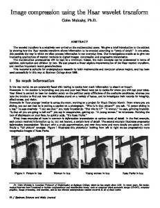
Fig 1: Modified Wavelet Transform with Edge Adaptation used for the next scale. The modified wavelet transform implementation is depicted in Figure 1. In 2D after edge detection we are end up with piecewise smooth regions with closed contours. The modified wavelet transform is applied to each region as the standard 2D separable wavelet transform is done where low and high pass filters are applied first on the rows then on the columns and this structure is repeated on the low-low image until the desired scale is reached. 4. RESULTS In order to show how the modified wavelet transform works, we provide performance results both for a 1D signal and an image. The 1D signal is the vertical scan line at the 204th column of the moon.tif image and shown in Figure 2, top plot. As it can be seen from Figure 2, bottom plot, its sigmafiltered version is smoother and weak edges are wiped out.

For comparison purposes we computed 7-level standard wavelet transform on the original 512 length signal which produces again four low pass coefficients and the rest are high pass coefficients. Both of the resulting transform coefficients are sorted in descending order. Then the signals are reconstructed using those sorted transform coefficients starting from 1 to 512. The distortion measure used is σ2d/σ2s where σ2d is the energy between the reconstructed and original signals and σ2s the energy of the original signal. The performance can be seen in Figure 3. The wavelet filters used are dB5, length 10 Daubechies filters. Only the performance up to 80 samples is shown since already zero distortion is reached. The modified transform performs better all the time but its superiority is clear when a few number of coefficients are used for reconstruction. That supports our idea of designing edge adapted wavelet transform.

modified, dB5 standard, dB5

0.25

250 200

0.2

150

50 0

0

100

200

300

400

500

600

Distortion

100

0.15

0.1

250 200

0.05

150 100 50 0

0 0

100

200

300

400

500

600

Figure 2: (top): Vertical scan-line of the original moon image, at x2=204. (bottom): Same scan-line of the sigmafiltered moon image. The edge points are detected using the sigma-filtered signal. They are found at points 87, 351, and 410, respectively. Since there are three edge points we have four signal segments. The resulted transform coefficients consist of one low pass coefficient and the rest are high pass coefficients for each segment.

10

20

30 40 50 Number of Samples

60

70

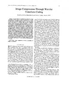
Figure 3: The performance comparison of modified and standard wavelet transform. We expect more gain in 2D. In order to show that we take the synthetic moon image shown in Figure 4, top. It is sigma filtered and then closed edge curves are detected. For complexity purposes only two edge curves are selected here. The edge curves are plotted in Figure 4, bottom. For performance comparison we computed the 3-level separable 2D standard and modified wavelet transforms, and the finite ridgelet transform [10].

rameter or in the edge deciding part by morphological processing. Finally, since the image consists of multi regions with different properties, the application at hand can be modified for every region differently. REFERENCES image

edge curves

Figure 4: (top): Moon image of size [256x256]. (bottom): Edge curves after sigma-filtering as described in the end of Section 3. The wavelet filters used are dB4, length 8 Daubechies filters. All three transforms’ non-linear approximation powers are evaluated in terms of signal-to-noise ratio (SNR) for comparison by using the N largest transform coefficients to reconstruct the original image. The results can be seen in Figure 5. From top to bottom, the first curve is the transform coefficients of the modified wavelet transform, the second curve is the transform coefficients of the standard wavelet transform and the third curve is the transform coefficients of the finite ridgelet transform, respectively. It is seen clearly that the modified wavelet transform achieves better performance than the others. This applies to image compression since it is done after thresholding very small transform coefficients. Since the moon image used for comparison does not have straight edges, the performance of the finite ridgelet transform is poorer.

[1] M. Vetterli, "Wavelets, Approximation, and Compression,'' IEEE Signal Proc. Magazine, pp. 59–73, Sept. 2001. [2] E. J. Candes, and D. L. Donoho, "Ridgelets: A Key to Higher-Dimensional Intermittency?,''Phil. Trans. R. Soc. London A, pp. 2495–2509, 1999. [3] J. L. Starck, E. J. Candes, and D. L. Donoho, "The Curvelet Transform for Image Denoising,'' IEEE Trans. Image Proc., vol. 11, pp. 670–684, June. 2002. [4] M. N. Do, and M. Vetterli, "Contourlets: A New Directional Multiresolution Image Representation,'' in Proc. IEEE Int. Conf. on Image Proc.(ICIP), 2002, pp. 497–501. [5] D. L. Donoho, "Wedgelets: Nearly-Minimax Estimation of Edges,'' Ann. Statist., vol. 27, pp. 859–897, 1999. [6] L. Pennec, and S. Mallat, "Image Compression With Geometrical Wavelets,'' in Proc. IEEE Int. Conf. on Image Proc. (ICIP), 2000, pp. 661–664. [7] A. Cohen, and B. Matei, "Compact Representation of Images by Edge Adapted Multiscale Transforms,'' in Proc. IEEE Int. Conf. on Image Proc. (ICIP), 2001, Thessaloniki, Greece, pp. 8–11. [8] R. Claypoole, G. Davis, W. Sweldens, and R. Baraniuk, "Nonlinear Wavelet Transforms for Image Coding,'' in Proc. 31st Asilomar Conf. on Signals, Systems, and Computers, 1997, pp. 662–667 [9] C. Kuo, and A. H. Tewfik, "Multiscale Sigma Filter and Active Contour for Image Segmentation,'' in Proc. IEEE Int. Conf. on Image Proc. (ICIP), 1999, pp. 353–357. [10] www.ifp.uiuc.edu/~minhdo/software/ FRIT_Toolbox

5. CONCLUSION 40

35

30 SNR(dB)

We have shown an edge adapted wavelet transform applicable to image compression. That is done by first detection the edge curves on the sigma-filtered image and then modifying the wavelet transform accordingly based on the edges present in the image. Better performances are observed both for 1D and 2D as shown with examples. As described in related sections the modified wavelet transform consists of two parts; shape information (edge curves) and transform coefficients for each region. We only deal here with the latter part although for practical image compression applications former part also has to be coded separately. As a result bit budget should be efficiently shared between shape information and transform coefficients for coding. There is a trade off between these two parts. We don’t want to spend the bit budget for a relatively complex shape if the transform coefficients from the region inside the shape do not result in high gain in reconstruction. In this respect the chosen curves might be chosen to be certain easy to code shapes. Similarly, regions with relatively small areas should be ignored and not coded separately. This can be done in the sigma filtering part by tuning the threshold pa-

25 modified wavelet transform, dB4 standard wavelet transform, dB4 finite ridgelet transform, dB4

20

15

4

6

8

10 12 14 16 Percentage of Retained Coefficients (x1/1000)

18

20

Figure 5: Comparison of non-linear approximations of the image in Figure 4, top, using the modified and standard 2D separable wavelet transforms and the finite ridgelet transform.