Edge-Region Integration for Segmentation of MR Images - BMVA

Edge-Region Integration for Segmentation of MR Images Gavin J. Brelstaff \ Michael C. Ibison fc Peter J. Elliott IBM UK Scientific Centre, Athelstan Ho, St Clement St, Winchester, Hants, SO23 9DR

A data-driven segmentation scheme is described that integrates edges and smooth regions. Edges are detected first and then used to guide the action of a dualresolution agglomeratine •parametric region detector. The scheme is applied to a variety of MR images. A comparison is made of segmentations produced by the scheme and by medical experts. The results are better than those obtained from the edge detection process alone.

This paper is a summary of recent work on edge-region based segmentation with particular application to magnetic resonance (MR) images of the brain. The objective to produce a model-free (or data-driven) segmentation useful for clinical diagnosis and treatment is one of our goals as a participant in an EEC funded project: Computer Vision in Radiology (COVIRA), which is part of the Advanced Informatics in Medicine (AIM) programme 1. As part of this programme we have been provided with a set of MR images manually segmented by medical experts (diagnostic radiologists) with which we can compare our results. The aim of this paper is to demonstrate a method for integration of two particular low-level primitives: Edges foiind by the Canny algorithm [2], and smooth regions found by the Silverman and Cooper algorithm [18]. MR images serve as a useful, i.e. particularly testing, domain upon which to demonstrate our method.

Literature Survey Below is a brief survey of existing algorithms for datadriven image segmentation. More extensive surveys are available [7]. Most existing algorithms are either edge detectors which mark discontinuities in the image intensity, or region detectors which mark homogeneous areas in the image.

provides an entirely satisfactory segmentation alone. We follow others [12,16,19] by integrating the two processes in an attempt to improve the overall segmentation. The two processes are in a sense complementary: edge detection exploits the local spatial support around each potential edge point while regions can be detected using the semi-global support across each potential region. Traditionally edge detection has been a process of locating points of maximum grey-level gradient [8,17]. We use the Canny operator to do this [2]. It provides the optimal trade off of the signal to noise ratio and the accuracy in locating edges. It leaves gaps at 2D features such as corners and junctions. Sometimes these gaps can be filled [11,9], otherwise it is our region detector's job to fill them. Many region detection algorithms are based on histogram splitting—see [7]—but these fail if any two regions to be distinguished contain the same grey-levels. If the two regions do not abut then spatially adaptive histogram splitting can work [3,20,13]. Patch fitting [21,1,18] provides a way to detect such regions even when they abut. Regions are detected on the basis of how well they fit to parameterised patches, each of which models an area of smoothly varying grey-level. We use a patch fitter that permits constant, planar or bi-quadratic fits [18]. It merges small regions into large ones using a maximum likelihood criterion. Alternative patch fitting strategies have been investigated: split and merge [15,10], parallel pixel growth [1], and searches for the M.A.P. segmentation using Gibbs random fields [4,14]. In all these schemes the spatial support for the detection of a region increases as the region grows. This contrasts with the purely local support exploited by Haralick's facet fitting edge detector [5,6].

Broad Outline of Method Our approach to integration is to use the results from an edge detection process to guide the action of an agglomerative clustering process.

In practice neither edge detection nor region detection 'G.J.Brelstaff now at PSRC, Dept of P»ychology, The Univer«ity, 8-10 Berkeley Square, BRISTOL, BS8 1HH. 'We thank Prof. F. Galvez and Dr. M. De»co of the Gregorio Maranon General Hospital, Madrid for providing the MR images and manual segmentations. Also thanks to the other collaborators within the COVIRA project for useful and interesting debate.

Edge detection Edge detection is accomplished through an implementation of the Canny algorithm, with non-maximal suppres-

139

BMVC 1990 doi:10.5244/C.4.26

sion, hysteresis [2] and junction completion [11].

lated to fill the tessellation tile they occupy so that agglomeration, inhibition (at edges), seeding, and termination (at new edges) can all take place at tile resolution. Thus the method described so far yields coarse boundaries with a spatial granularity equal to that of the tile

Serial Clustering The Silverman and Cooper method for growth of smooth grey-level patches has been adapted as follows: • Following the initial tessellation (into 'tiles'), agglomerative clustering is serial rather than parallel: each patch is grown from a seed point to completion, one patch at a time.

The next stage assigns pixels within the boundary tiles to patches according to the following recipe: • Assignment takes place only to adjacent patches.

• Completion is determined by the likelihood ratio stopping criterion described in [18].

• Only those unassigned pixels which are not adjacent to two different patches are considered.

• The current patch is constrained during growth to agglomerate only adjacent tiles which do not straddle a Canny edge, or an edge as inferred by the extent of a previously completed patch.

• The order of assignment is determined by a best fit calculation for each unassigned pixel to its adjacent patch. • The best fit minimises the difference between the pixel grey-level, and that implied by an extrapolation of the parametric grey-level surface of the adjacent patch.

Motivation: The idea here is to encourage the detection of closed regions which are largely bounded by credible but incomplete Canny edges. The support for edges added by the agglomerative method is thereby one-sided, giving rise to an improved signal to noise ratio.

• Patch parameters and adjacency are updated after each assignment.

Seeding The completion of a patch triggers a fresh cycle which begins with the determination of the next seed point until every tile is a member of a patch. Seed points are chosen according to the following method:

Motivation: Single pixel resolution for the final segmentation is obviously desirable. However, there is a signal to noise advantage from patch growth using enhanced local support, and therefore single pixel manipulations must be delayed as long as possible. Note that the second ingredient ensures that a one pixel wide boundary of unassigned pixels remains between different patches. We denote these as the new ('high resolution') edge points.

• Edge termination points found by the Canny process are recorded prior to all patch growth. • A record is updated at the beginning of each cycle of all 'free' edge points (originating from Canny or from a previoiisly completed region boundary) which are eight-way connected to at least one unassigned tile.

Merging similar patches A patch-patch merging process can be performed as follows:

• The next seed is (any) unassigned tile adjacent to a free edge point which is furthest from its nearest termination point.

• A goodness of fit is calculated for all possible (between adjacent patches) pair-wise merges. • The best merge is performed, and the patch parameters and adjacencies updated.

Motivation: Areas near edge terminals are the most likely to yield plausible new edges not found by the Canny edge detector. The hope is that the growing patch will approach this area with a low variance for the parametric fit, and therefore a high sensitivity for the detection of a difficult edge. The low variance is a consequence of getting off to a good start in a relatively (parametrically) homogeneous area, which should be as large as possible, before (one sidedly) encountering the piitative edge.

• The cycle is repeated until a stopping criterion (a threshold on the similarity) is met. Motivation: It is possible that a (parametrically) homogeneous patch of the image is split up into two or more patches even though there exists no unbroken Canny edge between them. This can arise when Canny edges conspire to form a bottle-neck through which the growing Silverman and Cooper patch cannot pass. For this reason, following the high resolution stage of patch growing, patches thereby brought into contact across (single pixel

High resolution (extrapolation) Prior to serial patch growing, Canny edge points are di-

140

relating optimal thresholds to global image parameters (noise, SNR) and (c) numerical: multidimensional conjugate gradient minimisation with objective: the total number of non-coincident edge points between the manual and automatic segmentations. We hope shortly to report both on the sensitivity of the objective around the minimum with respect to changes in threshold and image parameters, and the sensitivity of the optimal thresholds with respect to changes in global image parameters.

width) edges can be tested for similarity and merged accordingly.

Merging dissimilar patches Although parametrically dissimilar, two patches may be considered for merging based on other contextual information. It is our future intention to partition such actions into a separate process, wherein the rules governing such merges are made explicit. Meanwhile, we currently merge adjoining patches which have less than some small number of Canny edge points separating them.

Application to MRI

Summary of Algorithm

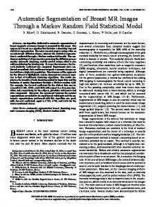
Image data Our MR images are 256x256x8 bits Tt and T2 weighted transaxial slices of the brain: Fig. 1, 2. The SNR is about 15dB. At present, our method is single channel, 2 dimensional. Therefore we consider each slice independently, and work with either Ti, T2 or the mean (Ti +T 2 )/2 image, which is often better. We have been provided with a set of manual segmentations by diagnostic radiologists with which we can compare our results: Fig. 7. Broadly speaking, we would like our results to be as close as possible to these.

• Edge detection - CANNY and HYSTERESIS - JUNCTION COMPLETION • Region detection - SERIAL CLUSTERING / SEEDING - EXTRAPOLATION - PARALLEL CLUSTERING

Application notes

(The last stage codes for clustering of both similar and dissimilar patches.)

The criterion of diagnostic usefulness demands that the segmented MR image be largely composed of closed regions which correspond to clinically distinct regions of the brain. Where we are likely to fail in this task, we err on the side of over-segmentation, mindful of possible future work on automatic interpretation with the segmentation results as an input.

Thresholds The various thresholds/parameters for controlling the processes described above can be manipulated in favour of the desired segmentation. To this end, we consider only:

Examination of the MRI grey-level surface reveals few clinically distinct regions which would benefit from a biquadratic parameterisation of patches. Indeed, so far we have been unable to show the benefit of using a bi-linear parameterisation rather than constant patches, despite in some cases an obvious partial volume effect near region boundaries. At least for our data set, we conclude that it is better to \ise the grey-level data within a tile to increase the SNR for detection of simple grey-level discontinuities, rather than use it to establish a higher-order parameterisation and therefore sensitivity to higher order discontinuities.

t The standard deviation of the Gaussian smooth performed by CANNY. • The upper and lower thresholds required by HYSTERESIS. • The degree of polynomial used to parameterise the patches for SERIAL CLUSTERING. • The percentage type 1 error expected (Silverman ans Cooper) on completion of the SERIAL CLUSTERING. • The acceptable fitting error for EXTRAPOLATION.

Results and discussion Fig. 1 shows a transaxial Tj slice taken from a patient with a temporal astrocytoma. The patient was treated with Gadolinium to enhance the outline of the tumour, which shows up as a bright ring. The tumour is surrounded by edema (swelling) which is not very well differentiated from the surrounding tissue. Fig. 3 gives the result of edge detection showing that the tumour boundary is found, but only part of the edema boundary. Fig. 4 is the result after region growing, showing that the region

• The minimum number of Canny edge points required to prevent PARALLEL CLUSTERING. Some work has been done on the optimal choice of thresholds which minimise the difference between the automatic and manual segmentations. Our approach has been (a) empirical (trial and error), (b) theoretical:

141

grower has successfully completed the edema boundary. Note also that the outlines of the skin, skull and brain are well defined, since they produce strong edges that are easily detected.

detection ofleft ventricle from cineangiograms. Comput. Biomed. Res. 5, 338-410, 1972. [4] Derin, H. and Elliott, H. Modeling and Segmentation of Noisy and Textured Images Using Gibbs Random Fields. IEEE Trans. PAMI 9, 39-55, 1987.

Fig. 2 is the [T\ + Tz)/2 image from, a transaxial slice of another patient (without the use of Gadolinium). In this case there is a frontal solid astrocytoma, with very little edema. Fig. 5 shows the results of edge detection, with the same thresholds as in the previous example. Fig. 6 shows the completed edges after region detection. For this image, a manual segmentation was performed by diagnostic radiologists, with a criterion of clinical usefulness. This is shown in Fig. 7, and enables us to get a measure of how well the computer algorithms have performed. In the manual segmentation, there are 3959 edge points, compared to 5440 in the computer segmentation (recall that over-segmentation is preferred to an undersegmentation). Of these, 1591 edge points or 40% of the total in the manual segmentation are coincident. There are only 658 of the manual edge points which are more than one pixel from a computer generated edge point i.e. 84% of the manual segmentation has been identified, within 1 pixel, by the computer segmentation. This is shown in Fig. 8.

[5] Haralick, R.M. Edge and Region Analysis for Digital Image Data, CGIP 12, 60-73, 1980. [6] Haralick, R.M. Digital Step Edges from ZeroCrossings of Second Directional Derivatives IEEE Trans. PAMI, 6, 58-68, 1984. [7] Haralick, R.M. and Shapiro, L.G. Image Segmentation Techniques. CGVIP 29, 100-132, 1985. [8] Hueckel, M.H. A local visual operator which recognizes edges and lines. J. A.CM. 20, 4, 634-647, 1973. [9] Lacroix, V. A Three-Module Strategy for Edge Detection, IEEE Trans. PAMI, 10, 803-810, 1988. [10] Laprade and Doherty. Split and merge segmentation using an F-test criterion. Image Understanding and the Man-Machine Interface, SPIE Vol. 758, 1987.

It can be seen that in addition to the skin, skull and brain outlines, a large part of the grey/white matter boundary has been correctly identified (this is often difficult to detect). Also the boundary of the tumour has been found correctly. In the centre of the image, the ventricular area, the overall outline of the structure is quite well defined. However, the separation of the ventricles from the nucleus caudatus has been lost, as can be seen from the manual segmentation. Note that the radiologists iise their anatomical knowledge when performing the segmentation, in contrast with our piirely data-driven approach. Using the same value for the thresholds, so far we have apphed our technique for segmentation to 25 images from 6 patients with good results. In summary, the edge-region, based scheme described above has performed useful segmentations in the particularly difficult domain of MR images. The results obtained by integrating the edge and region detection processes are better than those that are achieved by edge detection alone.

References [1] Besl, P J . and Jain, R.C. Segmentation Through Variable-Order Surface Fitting. IEEE Trans. PAMI, 10, 2, 167-192, 1988. [2] Canny, J . F . Finding edges and lines in images. S.M. thesis, MIT, Cambridge, USA, 1983. [3] Chow, C.K. and Kaneko, T. Automatic boundary

[11] Li, D., Sullivan, G.D. and Baker, K.D. Edge Detection at Junctions. Proc. AVC, 121-125, 1989. [12] Nazif, A.M. and Levine, M.D. Low Level Image Segmentation: An Expert System, IEEE Tram. PAMI, 6, 555-577, 1984. [13] Ohlander R., Price, K. and Reddy, D.R. Picture segmentation using a recursive region splitting method. CGIP 8, 313-333, 1978. [14] Pappas, T.N. and Jayant, N.S. An Adaptive Clustering Algorithm for Image Segmentation. Proc. 2nd Int. Conf. Compui. Vision, Florida. 310-315, 1988. [15] Pavlidis, T. Structural Pattern Recognition. SpringerVerlag, New York, 1977. [16] Pavlidis, T. and Liow, Y.T. Integrating Region Growing and Edge Detection, Proc. Conf. Comp. Vis. Palt. Recog. 208-214, 1988 [17] Prewitt, J.M.S. Object Enhancement and Extraction, in Picture Processing and Psychopictorics, Lipkin, B.S. and Rosenfeld, A., Eds., Academic Press, New York, 75-149, 1970. [18] Silvermaii, J . F . and Cooper, D.B. Bayesian Clustering for Unsupervised Estimation of Surface and Texture Models. IEEE Trans. PAMI 10, 482-495, 1988. [19] Wrobel B. and Monga, O. Segmentation d'images naturelles: Cooperation entre un detecteur-contour et un detecteur-region, Acies du 11th Colloque GRETSI, Nice, France, June 1987. [20] Yanowitz, S.D. and Bruckstein, A.M. A New Method for Image Segmentation. CVGIP, 46, 82-95, 1989. [21] Yakimovsky, Y. Boundary and object detection in real world images. J. Assoc. Comput. Mach. 23, 599618, 1976.

142

Figure 1: MR image of the brain: transaxial Tx slice exhibiting a temporal astrocytoma ( the bright ring), enhanced by Gadolinium treatment.

Figure 3: Canny edges from Fig. 1.

Figure 2: MR image: transaxial slice exhibiting a frontal solid astrocytoma (bright blob)-the average of Ti and T5 weighted images.

Figure 4: Seeded region growing on Fig. 1 guided by the Canny edges (Fig. 3).

143

Figure 5: Canny edges from Fig. 2.

Figure 7: Manual segmentation performed by a diagnostic radiologist—to be compared with the computed segmentation in Fig. 6.

Figure 6: After region growing on Fig. 2 using edges in Fig. 5.

Figure 8: Image showing the 84% of the manual segmentation (Fig. 7) identified by the computed segmentation in Fig. 6.

144