Boyu Wang, Feng Wan, Peng Un Mak, Pui In Mak, and Mang I Vai. Department of Electrical and Electronics Engineering. Faculty of Science and Technology.
EEG Signals Classification for Brain Computer Interfaces Based on Gaussian Process Classifier Boyu Wang, Feng Wan, Peng Un Mak, Pui In Mak, and Mang I Vai Department of Electrical and Electronics Engineering Faculty of Science and Technology University of Macau Macau Abstract—Classification of electroencephalogram (EEG) is a crucial issue for EEG-based brain computer interface (BCI) system. In this paper, the performances of the Gaussian process classifier (GPC) for three different categories of EEG signals, i.e. steady state visually evoked potential (SSVEP), motor imagery and finger movement EEG data, are investigated. The main purpose of this paper is to explore the practicability of GPC for EEG signals classification of different tasks. Compared with some commonly employed algorithms, the GPC achieves similar or better performances. Furthermore, the probabilistic output provided by the GPC can also be of great benefit to the decision making for both online and offline EEG analysis. Keywords-Gaussian process classifier (GPC), brain computer interface (BCI), electroencephalogram (EEG)
I.
INTRODUCTION
The brain computer interface (BCI) can provide a communication channel from a human to a computer which enables the brain to send messages without using traditional pathways as nerve or muscle [1]. The ultimate purpose of a direct BCI is to allow an individual with severe motor disabilities to have effective control over devices such as computers, speech synthesizers, assistive appliances and neural prostheses [2]. In general, a BCI system detects the patterns of brain activity and translates them into sequences of control commands. At present, the brain activities are often recorded noninvasively by electroencephalogram (EEG), which has excellent temporal resolution and usability, and the EEG signal is therefore the most popular choice for BCI research. One crucial and challenge issue for EEG-based BCI system is the classification of EEG signals. Overall, the linear classifiers, e.g. linear discriminant analysis (LDA), are recommended wherever possible. However, if regularization is applied, nonlinear methods, e.g. nonlinear support vector machine (SVM) can also provide desirable results especially with complex nonlinear EEG data set [3] [4]. But the methods using regularization also lead to the awkward problem of how to set the penalty parameters (e.g. the parameter α in the weight regularization term α w T w for a weight vector w ) [5]. For Gaussian process (GP) model, the tradeoff between penalty parameters and data-fit is automatic. There is no need to set a weighting parameter by some external method to fix the
978-1-4244-4657-5/09/$25.00 ©2009 IEEE
tradeoff, and the training of a GP model is referred to the selection of a covariance function and its parameters (hyperparameter) [6]. In addition, superior to other commonly applied classifiers in the BCI community, the Gaussian process classifier (GPC) can provide the probabilistic outputs, which will benefit the decision making for both online and offline EEG analysis. The performance of GPC for motor imagery EEG signals was well studied in [9]. To further investigate the usability of GP model for EEG-based BCI system, the GPC is applied to three categories of EEG signals, i.e. steady state visually evoked potential (SSVEP), motor imagery and finger movement EEG data. The GPC is also compared with other commonly employed classifiers in BCI community. In addition, the three kinds of EEG raw data are processed by different feature extraction strategies respectively to improve the classification accuracy. II.
GAUSSIAN PROCESS CLASSIFIER
A. Gaussian Process for Regression A Gaussian process is a collection of random variables, any infinite number of which have a joint Gaussian distribution [6]. The Gaussian distribution is over vector, whereas the Gaussian process is over functions, which means a Gaussian process is completely specified by its mean function μ ( x) = E[Y ( x)] and covariance function k ( x, x ') = E[(Y (x ) − μ (x ))(Y ( x ') − μ (x '))] [7]. Similar to SVM, there are many kernel functions which can be used as covariance function for Gaussian process. A widely employed form is
k (x, x ') = θ 0 exp{−
1 d ∑ wl ( xl − xl ')2 } + θ1 2 l =1
(1)
where xl is the lth component of x and θ = (θ 0 , θ 0 , w1 ,..., wd ) is the set of positive hyperparameter of covariance function. Given a set of training data D = {(xi , ti ), i = 1, 2...n} , our goal is to predict the real valued output y* = y ( x* ) for new input x* . From the definition of a Gaussian process, given a set of inputs x1 ,…, x n , we can specify the prior over corresponding
ICICS 2009
output as P( y ) , where y = ( y (x1 ),..., y (x n ))T . For simplicity the mean function μ ( x) is usually taken to be zero, i.e. μ (x ) ≡ 0, so that P(y ) = N (0, K ) where [K ]ij = k ( xi , x j ) ,We can also take account the noise on the observed value, which given by ti = yi + ε i where yi = y ( x i ) , and ε i is a random variable. One common assumption is that of additive i.i.d Gaussian additive noise with mean zero and variation σ 2 in the outputs, so that P (t | y ) = N ( y , σ I ) 2
where t = (t1 ,..., tn ) and the marginal distribution P (t ) is therefore given by
P(t ) = ∫ P(t | y ) p (y )dy = N (0, K + σ 2 I ) To predict the target value y* for the new input x* , we need to calculate the predictive distribution
P( y* | t ) = ∫ P( y* , y | t )dy =
1 P ( y* | y ) P(y ) P (t | y )dy P (t ) ∫
(4)
In general, since L is a not convex function, there may be local maxima in the likelihood surface. In a Bayesian treatment, we can define a prior distribution over the set of hyperparameters θ and then evaluate the marginals over θ by the product of the prior P(θ) and the likelihood function P(t | θ) . For Gaussian process, the marginalization is intractable, but the numerical method could be used to approximate the integration [8]. B. Gaussian Process for Classification The output of a GP model lies on the entire real axis. Using a proper transfer function, however, we can produce an output lie in the interval (0,1), which can be interpreted as the probability of class 1. For binary classification, one common choice for the transfer function is logistic function y = σ (a ) , where σ (a ) = 1/(1 + e − a ) . Instead of Gaussian distribution in the regression case, the probability distribution over the target value t ∈ {0,1} for classification task is given by Bernoulli distribution, i.e. t ∼ Bern(σ (a )) . To make the prediction for two-class problems, we need to calculate the predictive distribution
(2)
= ∫ P ( y* | y ) P(y | t )dy
P(t* = 1| t ) = ∫ P(t* = 1 | a* ) P(a* | t )da* = ∫ σ * P (a* | t )da*
It should be noted that P( y* | t ) is also the conditional distribution on x1 ,…, x n and x* [8]. To keep the notation simple the conditioning variables are shown implicitly. Since the prior and the noise model are both Gaussian, the integral of the product of them is also Gaussian. Therefore, for a specific test data x* , the posterior is given by P( y* | t ) = N (m* , σ *2 ) , m* = k *T K −1t
(5)
where a* = a (x* ) , and σ * = σ (a* ) . Unlike the regression case, this integration is no longer analytically intractable, so sampling or approximation methods, e.g. the Markov chain Monte Carlo (MCMC) methods, expectation propagation, variational Bayes, and the Laplace approximation, can be used. It has been shown that the GPCs based these methods have the similar performances with the motor imagery EEG data [9]. Therefore, we only employ the Laplace approximation here and briefly describe it below. Eq. (5) can be approximated by the following formula [8]:
σ *2 = k** − k T* K −1k * where K = K + σ I , k * = (k (x* , x1 ),..., k (x* , x n )) , and k** = k (x* , x* ) . 2
⎛ ∂L 1 ∂K ⎞ 1 T −1 ∂K −1 K t = − trace ⎜ K −1 ⎟+ t K 2 ∂θ i ∂θ i ⎠ 2 ∂θ i ⎝
T
To make prediction for a new test data, we also need to infer the set of hyperparameters from the training data by either making a point estimate or resorting to Bayesian approach where a posterior distribution over the parameters is obtained [7]. The calculations are based on the log marginal likelihood function log P(θ | t ) . For Gaussian process regression, the distribution of data is also Gaussian 1 1 n L = log P (θ | t ) = − log | K | − tT K −1t − log(2π ) 2 2 2
(3)
Then we can find the optimal hyperparameters which maximize the log marginal distribution based on its partial derivatives
∫ σ (a ) N (a | μ , σ
2
)da
σ (κ (σ 2 ) μ )
(6)
where κ (σ 2 ) = (1 + πσ 2 / 8) −1 / 2 . This requires that we have a Gaussian approximation to the posterior distribution P( a* | t ) . However, since P(t | a ) = σ ( a)t (1 − σ (a ))1− t , even though the we use a GP prior over ( a* , a) , where a = (a (x1 ),..., a( x n )) , P( a* | t ) is analytically intractable. Using Bayes’ theorem, we have P(a* | t ) = ∫ P(a* | a)P(a | t )da
(7)
where P( a* | a) = N (k T* K −1a, k** − k T* K −1k * ) . Therefore, we can approximate the Eq. (7) by finding the Laplace approximation for the posterior distribution P(a | t ) , and therefore we need to
find the modal value of P(a | t ) . This can be done by maximizing ψ = log P(a) + log P (t | a) with respect to a . Using
log P (ti | ai ) = ti ai − log(1 − e ai ) , where ψ is given by ψ = log P(a) + log P(t | a) n
1 1 n = − aT K −1a − log | K | − log(2π ) + tT a − ∑ log(1 + eai ) 2 2 2 i =1
(8)
Differentiating (8) with respect to a , we obtain ∇ψ = t − σ − K −1a where σ = (σ ( a1 ),..., σ ( an ))T . ∇∇ψ = − W − K −1 where W = diag (σ ( a1 )(1 − σ (a1 )),..., σ ( an )(1 − σ (an ))) , which give the iterative update equation for a : a new = ( W + K −1 ) −1 ( Wa + t − σ )
(9)
Having found the converged solution aˆ for a , we can specify the Laplace approximation to the posterior distribution P (a | t ) as P (a | t )
q (a ) = N (aˆ , ( W + K −1 ) −1 )
(10) where the elements of W are evaluated using aˆ . Combining (10) with (7), the mean and the variance of a* is given by E[a* | t ] = k T* (t − σ ) Var[a* | t ] = k** − k T* ( W −1 + K )−1 k * Then using (6) we can approximate the integral (5), and make the decision according the result. We also need to adjust the set of hyperparameters θ for GPC, which involves the likelihood function P(t | θ) :
∫
P (t | θ) = P (t | a)P(a | θ) dθ
(11)
Again by using the Laplace approximation, the log of P ( t | θ ) is given by
log P (t | θ)
1 n ψ (aˆ ) + log | W + K −1 | + log(2π ) 2 2
(12)
Then similar with the GP regression, the parameters can be learned by either maximizing the likelihood function P(t | θ) or resorting to Bayesian approach, e.g. [7] [10]. III.
EXPERIMENTS
A. Data Sets To investigate the practicability of GPC for EEG-based BCI, the GPC is applied to three categories of EEG signals, i.e. motor imagery finger movement EEG data, and steady state visually evoked potential (SSVEP). The first two data sets are
dataset III and IV in BCI competition 2003 [15], which are provided by Graz BCI group and Fraunhofer-FIRST, Intelligent Data Analysis Group; Freie Universität Berlin, Neurophysics Group respectively. Dataset III was recorded from a 25 years old female during a feedback session. Three pairs of bipolar EEG channels (anterior ‘+’, posterior ‘-’) were positioned over C3, Cz and C4. It was sampled at 128 Hz and bandpass filtered between 0.5 and 30Hz. This dataset consists of 280 trials (140 left trials and 140 right trials) of 9 s length. In each trial, the first 2s was quite. At 3s, an arrow (left or right) was displayed as cue while the female was asked to imagine left or right hand movement according to the cue. One half of dataset (140 trials: 70 left trials and 70 right trials) are used to training the BCI system, the others are used to testing. Dataset IV was recorded from a normal subject during a nofeedback session. The task is to press with the index and little fingers the corresponding keys in a self-chosen order and timing ‘self-paced key typing’. The EEG was collected by 28 electrodes at the positions of the international 10/20-system. The duration of the signal is 500ms ending 130 ms before a keypress, and the sample rate was 100Hz. There’re 416 trials in the dataset, including 316 training trials and 100 testing trials. In addition, we also investigated the performance of GPC for SSVEP, and the data set was from our own experiment. Four healthy, male, right-handed adults with normal or correctto-normal vision participated in the experiment. Subjects were seated 50cm from two simultaneously flickering white light emitting diodes (LED) modulated by square waves. Since our aim is to verify the usability of GPC for EEG-based BCI system and compare the performance of GPC with other commonly used classifier, e.g. LDA and SVM, which are originally designed for binary classification, we only generate two integer frequencies, i.e. 14Hz and 15Hz. The experiment contained 4 trials containing 40 trials each, i.e. for each subject, there are 80 trials (40 trials for training and 40 trials for testing) for each frequency, and each trial lasted 6s. The subjects had 2s-break at the beginning of each trial. From 2s to 6s, the subjects were required to gaze one of the LEDs with a certain frequency. In every runs, each frequency, i.e. 14Hz and 15Hz was randomly indicated 20 times. EEG signals were recorded from O1 and O2 according to the international 10-20 system and referred to the left and right ear lobes respectively, and the sampling rate is 512 Hz.
B. Feature Extraction Due to the differences of the EEG signals, we applied different feature extraction methods. For motor imagery classification task (data set II), we introduced event-related desynchronization (ERD) [11] on the contralateral sensorimotor area during motor imagery. The data set III was sampled from 3 channels where are C3, Cz and C4, respectively. Only C3 and C4 channel data are employed here since the ERD feature in Cz is not clear. First, the C3 and C4 channel data is filtered by IIR (Infinite Impulse Response) bandpass filter (10-12 Hz). Then the two time courses of ERD ec3(k) and ec4(k) are computed at k-th sampling point by
equation (13) [16]. xc3(k) and xc4(k) are the filtered data from C3 and C4 channel, respectively, w −1
w −1
i =0
i =0
ec 3 (k ) = ∑ xc 3 (k − i ) 2 , ec 4 (k ) = ∑ xc 4 (k − i ) 2
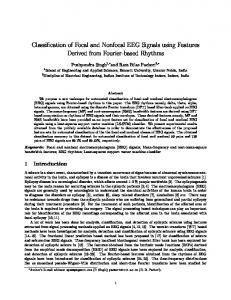
FM EEG data set. In addition, it achieves the higher classification accuracies for SSVEP (83.75%) and MI EEG data set (86.43%) than any other classifiers.
(13)
where w is the length of time window. In this experiment, we choose w = 15 (≈ 117.2 ms), and starting point of the time window is t = 560 (= 4.375s). Each feature vector ec(k) is constructed by two column vectors ec3(k) and ec4(k), where is denoted in (14).
ec (k , m) = [ec 3 (k , m), ec 4 (k , m)] (14) where k is denoted the k-th sampling point and m is denoted the m-th trial. For finger movement task, the features are extracted from bereitschaftspotential (BP), which is low-frequency potential that reflects the dynamic changes in motor cortical activity prior to the movement onset, and can be recorded with the maximum amplitude over the vertex region [12]. Before the feature extraction, the BP signals are first preprocessed by lowpass filter and temporal filter respectively. The cutoff frequency of the low-pass filter is 7Hz, and the starting point and the length of the time filter are t = 43 (200ms before the keypress) and w = 7 (60ms) respectively. Then common spatial subspace decomposition (CSSD) [13] is applied to extract the features. For SSVEP, the data are first filtered with a bandpass of 1050 Hz. For every 2s-6s of trial, the features are extracted by 2048 points fast Fourier transformation (FFT) every 0.25s (128 points) with 2s time window. The average values of the first three harmonics of each frequency are used as feature vectors for offline analysis and classification.
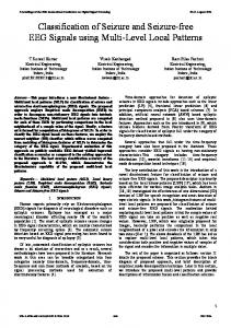
Figure 1. The classification accuracies for SSVEP of four subjects.
Figure 2. The performances of the classifiers for three types of EEG data.
V.
C. Parameter Selection For GPC, we need to determine the hyperparameters θ of the covariance functions, and we make the point estimation of θ , which maximize the likelihood function P ( t | θ). In addition, we also compare GPC with four other commonly employed classifiers in BCI community, i.e. LDA, linear SVM, nonlinear SVM (with Gaussian kernels) and backpropagation network (BPN). The optimal parameters of these classifiers are selected by 8-fold cross-validation on the training data, and the average classification accuracy is the criteria for choosing the optimal parameters of the classifiers. IV.
EXPERIMENTAL RESULTS
Figure 1 shows the performances of the classifiers for SSVEP of the four subjects, where LSVM and GSVM denote linear SVM and nonlinear SVM with Gaussian kernels. The performances for three types of data sets, i.e. SSVEP, motor imagery (MI), and finger movement (FM) EEG signals, are shown in Figure 2, where the classification accuracies of SSVEP are the average result of the four subjects in Figure 1. As observed in the two figures, the GPC in general has the similar classification accuracies with GSVM, which is superior to LSVM and BPN in all the data sets. On the other hand, the GPC also has better performances than the LDA except for the
DISCUSSIONS AND CONCLUSIONS
In this work, we verify the usability of the GPC for EEGbased BCI system. The GPC is compared with four other commonly employed classifiers in BCI community. The experimental results have demonstrated that GPC has desirable performances and outperforms LSVM and BPN in terms of the classification accuracy across all of the three types of EEG data set. Just like SVM, GPC is a flexible model which is insensitive to the curse-of-dimensionality, and the overfitting problem can be avoided due to the regularization property. Moreover, the tradeoff between penalty and data-fit in the GP model is automatic. Superior to SVM and LDA, the GPC can fit into Bayesian framework and naturally produces probabilistic outputs, which will benefit the decision making for both online and offline EEG analysis. Specifically, for the real time BCI system, if the posterior probabilities of a new test data are approximately equal to 0.5, we can reject this data and make no decision to avoid the occurrence of the false positive. This idea can also be extent to design of asynchronous BCI system, which analysis the EEG continuously and uses no cue stimuli [14]. Besides, GPC can also tackle the multiclass classification problem since the extension the binary classes GPC to multiple classes is straightforward.
Therefore, the GPC is recommended for BCI system, and our future work will focus on applying the GPC to the online EEG signal classification and developing reliable real time BCI system. ACKNOWLEDGMENT The authors gratefully acknowledge support from the Macau Science and Technology Department Fund (Grant FDCT/014/2007/A1) and the University of Macau Research Fund (Grant RG059/08-09S/FW/FST). REFERENCES [1]
[2]
[3]
[4]
[5]
J. R. Wolpaw, N. Birbaumer, D. J. McFarland, G. Pfurtscheller, and T. M. Vaughan, “Brain-computer interface for communication and control,” Clin. Neurophsiol., vol. 133, pp. 767-791, June 2002. A. Bashashati, M. Fatourechi, R. K. Ward, and G. E. Birch, ‘‘A survey of signal processing algorithms in brain-computer interfaces based on electrical brain signals,” J. Neural Eng., vol. 4, pp. R32---R57, 2007. K.-R.Müller, C.W. Anderson, and G. E. Birch, “Linear and nonlinear methods for brain-computer interfaces,” IEEE Trans. Neural Syst. Rehabil. Eng., vol. 11, pp. 165---169, June 2003. K.-R.Müller, M. Krauledat, G. Dornhege, G. Curio, and B. Blankertz, “Machine learning techniques for brain-computer interfaces,” Biomed. Technol., vol. 49, pp.11-22, 2004. C. K. I. Williams, “Prediction with Gaussian processes: from linear regression to linear prediction and beyond,” in Learning and Inference in Graphical Models, M. I. Jordan, Eds. Kluwer Academic Press, pp. 599621, 1998.
[6] [7]
[8] [9]
[10]
[11]
[12]
[13]
[14]
[15] [16]
C. E. Rasmussen, and C. K. I. Williams, Gaussian Processes for Machine Learning, The MIT Press, Cambridge, MA, 2006. C. K. I. Williams, and D. Barber, “Bayesian classification with Gaussian processes,” IEEE Trans. Pattern Anal. Machine Intell., vol. 20, no. 12, pp. 165---169, Dec 1998. C. M. Bishop, Pattern Recognition and Machine Learning, Springer Press, New York, 2006. M. Zhang, F. Lotte, M. Girolami, and A. Lécuyer, “Classify EEG for brain computer interfaces using Gaussian processes,” Pattern Recognit. Lett., vol. 29, pp. 354-359, Feb, 2008. D. Barber, and C. K. I. Williams, “Gaussian processes for Bayesian classification via hybrid Monte Carlo,” in Advances in Nerual Information Processing Systems 9, M. C. Mozer, M. I. Jordan, and T. Petsche, Eds, MIT Press, 1997. G. Pfurtscheller, and F. H. Lopes da Silva, “Event-related EEG/MEG synchronization and desynchronization: basic principles,” Clin. Neurophysiol., vol. 110, pp. 1842–1857, Nov. 1999. Y. Wang, Z. Zhang, Y. Li, X. Gao, S. Gao, and F. Yang, “BCI competition 2003 data set IV: an algorithm based on CSSD and FDA for classifying single-trial EEG,” IEEE Trans. Biomed. Eng., vol. 51, pp. 1081-1086, June 2004. Y. Wang, P. Berg, and M. Scherg, “Common spatial subspace decomposition applied to analysis of brain responses under multiple task conditions: a simulation study,” Clin. Neurophysiol., vol. 110, pp. 604614, Apr. 1999. G. Pfurtscheller, G. R.Müller-Putz, J. Pfurtscheller, R. Rupp, “EEGBased asynchronous BCI controls functional electrical stimulation in a tetraplegic patient,” J. Appl. Signal Process., vol. 19, pp. 3152–3155, 2005. BCI competition. Available: http://www.bbci.de/competition/ii/ W. Jia, X. Zhao, H. Liu, X. Gao, S. Gao, and F. Yang, “Classification of Single Trial EEG during Motor Imagery based on ERD,” in Proc. 26th Annu. Int. IEEE EMBS Conf. 2004, pp. 5-8.