Proc. of Int. Conf. onMultimedia Processing, Communication& Info. Tech., MPCIT
Effect of Adaptive Filters and Windowing Function on Bandwidth, Directivity and Time of Digital Beamforming Chirappanth B Albert1, Shashikumar.D* Dept. of ECE, Christ University, Faculty of Engineering, Kaniminike, Bangalore, India Email:
[email protected], *
[email protected]
Abstract— The antenna array exhibit flexibility in the design of radiation patterns. Conventionally, arrays are designed by controlling excitation levels, phase levels and space distribution of elements. In practice, for pre designed radiating elements in the array, one of the above parameters is considered for the design keeping the others fixed. When the elements of the array are uniformly excited, the first sidelobe level is found to be -13.5 dB. It is of interest here to reduce the sidelobe levels, increase the directivity by decreasing the beamwidth and also to reduce the time required to minimize the error minimization time using different window functions and adaptive filters. Index Terms - Directivity, Digital Beam Forming, Digital down Converter, LMS Algorithm, RLS Algorithm, RF Translator
I. INTRODUCTION There is an ever-increasing demand on mobile wireless operators to provide voice and high-speed data services. At the same time, these operators want to support more users per base station to reduce overall network costs and make the services affordable to subscribers. As a result, wireless systems that enable higher data rates and higher capacities are a pressing need. Smart antenna technology offers a significantly improved solution to reduce interference levels and improve the system capacity. With this technology, each user's signal is transmitted and received by the base station only in the direction of that particular user. This drastically reduces the overall interference in the system [1]. Digital beam forming (DBF) technology is progressed with the development of adaptive algorithms and architectures. Multiple Beam formation using the same antenna array is achieved by using the LMS algorithm. The performance criteria of a digital beam forming system are the number of antenna elements, the IF sampling rate, the RF frequency and the number of iterations required to converge. Least Mean Square (LMS) and Recursive Least Square (RLS) algorithms are being chosen to update complex weights to form the beam in the desired direction [7]. II. DIGITAL BEAMFORMING In digital beam forming, as all know the operations of phase -shifting and amplitude scaling for each antenna element, and summation for receiving, are done digitally. Either general-purpose DSP’s or dedicated beam forming chips are used [1]. Digital processing requires that the signal from each antenna element is digitized using an A/D converter. Since radio signals above shortwave frequencies (>30 MHz) cannot be directly digitized at a reasonable cost, so as a result the digital beam forming receivers uses the analog RF translators DOI: 02.AETS.2013.4.13 © Association of Computer Electronics and Electrical Engineers, 2013
to shift the signal frequency down before the A/D converters [2].
Figure1: Digital beam forming receiver
Once the antenna signals have been digitized, they are passed to digital down-converters that shift the radio channel’s centre frequency down to 0 Hz and pass only the bandwidth required for one channel [7]. The down-converters produce the quadrature baseband output at a low sample rate. The quadrature baseband inphase and quadrature components can be used to represent a radio signal as a complex vector (phasor) with real and imaginary parts. Here we need two components so that both the positive and the negative frequencies can be represented [5]. is the complex baseband signal is the real part is the imaginary part For beam forming, the complex baseband signals are multiplied by the complex weights to apply the phase shift and amplitude scaling required for each antenna element
Figure2: Complex multiplier
10
is complex weight for the antenna element is the relative amplitude of the weight is the phase shift of the weight A general-purpose DSP can implement the complex multiplication for each antenna element:
One set of antenna elements RF translators, and A/D converters can be shared by a number of beam formers. All RF translators and A/D converters share common oscillators. Within the digital beam former, all digital down-converters have common clock, and are set for the same centre frequency and bandwidth. Their digital local oscillators are in-phase so that all phase shifts are identical [5]. Each DDC baseband output is multiplied by the complex weight for its antenna element, and the results are summed to produce one baseband signal with directional properties. A demodulator would then follow to recover information. III. ADAPTIVE FILTER ALGORITHM The LMS and RLS Adaptive Algorithms :- The LMS (least mean squares) algorithm is an approximation of the steepest descent algorithm which uses an instantaneous estimate of the gradient vector (L.C. Godara, 1997).The task of the LMS algorithm is to find a set of filter coefficients c that minimize the expected value of the quadratic error signal, i.e., to achieve the least mean squared error . The basic idea behind LMS filter is to approach the optimum filter weights, by updating the filter weights in a manner to converge to the optimum filter weight [6]. The algorithm starts by assuming small weights and at each step, by finding the gradient of the mean square error (MSE), the weights are updated. That is, if the MSE-gradient is positive, it implies, the error would keep increasing positively, if the same weight is used for further iterations, which means we need to reduce the weights. In the same way, if the gradient is negative, we need to increase the weights [7]. The RLS (recursive least squares) algorithm is another algorithm for determining the coefficients of an adaptive filter. In contrast to the LMS algorithm, the RLS algorithm uses information from all past input samples along with the current samples to estimate the (inverse of the) autocorrelation matrix of the input vector. To decrease the influence of input samples from the far past, a weighting factor for the influence of each sample is used [7]. IV. WINDOWING TECHNIQUES Taylor, Hamming, Blackman and Uniform Window Functions Taylor window allows you to make trade-offs between the main lobe width and side lobe level. The Taylor distribution avoids edge discontinuities, so Taylor window side lobes decrease monotonically. Taylor window coefficients are not normalized. Taylor windows are typically used in radar applications, such as weighting synthetic aperture radar images and antenna design [3]. Hamming window is represented by
Blackman window is represented by
The uniform window is really no window at all. It is sometimes called the “boxcar function” because it looks like a boxcar, a pulse that is unity for all values of time [3].The uniform window provides the best frequency
11
resolution and amplitude accuracy, but can only be used if the measured signal is periodic in the time record. This condition is rarely met with naturally occur- ring signals, but can be met in controlled testing [6]. V. SIMULATION RESULTS When N=10
(a)
Directivity=8.0974; Beam Width =24.3000; Time Elapsed=15.309638 Sec
When N=14
(b) Directivity=9.4179; Beam Width =17.64000; Time Elapsed=20.465143 Sec Figure 3: Single Beam Radiation Pattern, Number of Iterations and Frequency Response for Hamming Window, Using LMS Algorithm at
and N=10 and N=14.
When N=10
(a) Directivity= 7.6271; Beam width =27.5400; Elapsed time is 7.028401 seconds
12
When N=14
(b) Directivity=9.4180; Beam Width =17.6400; Time Elapsed=17.888125 Sec Figure 4: Single Beam Radiation Pattern, Number of Iterations and Frequency Response for Hamming Window, Using RLS Algorithm at
for N=10 and N=14.
N=10
(a) Directivity= 7.6271; Beam width =27.5400; Elapsed time is 7.028401 seconds
N=14
(b) Directivity= 9.0878; Beam width = 19.2600; Elapsed time is 10.371368 seconds Figure5: Single Beam Radiation Pattern, Number of Iterations and Frequency Response for Blackman Window, Using LMS Algorithm at
for N=10 and N=14
(a) Directivity= 7.6272; Beam width = 27.5400; Elapsed time = 11.799713 seconds
13
(b) Directivity= 9.0879; Beam width = 19.2600; Elapsed time = 7.269231 seconds Figure 6: Single Beam Radiation Pattern, Number of Iterations and Frequency Response for Blackman Window, Using RLS Algorithm at
for N=10 and N=14
N=10
(a) Directivity= 9.3103; Beam width =18.3600;Elapsed time = 11.214846 seconds
N=14
(b) Directivity= 10.7705; Beamwidth = 12.9600; Elapsed time = 7.695792seconds Figure7: Single Beam Radiation Pattern, Number of Iterations and Frequency Response for Taylor Window, Using LMS Algorithm at for N=10 and N=14
N=10
(a) Directivity= 9.3103; Beam width = 18.3600; Elapsed time = 8.735426 seconds
14
N=14
(b) Directivity= 10.7705; Beam width = 12.9600; Elapsed time = 12.580070 seconds Figure 8: Single Beam Radiation Pattern, Number of Iterations and Frequency Response for Taylor Window, Using RLS Algorithm at for N=10 and N=14
VI. CONCLUSIONS The windowing techniques used here will provide cost effective solution compared to the uniform arrays. From simulation results it is evident that the sidelobe levels get reduced from -13.5 dB to -60 dB. The results show that the radiation patterns are getting converged at 200 iterations using LMS and 100 iterations using RLS thereby reducing the time required to reduce the error. It is also evident from the results that the beam width gets reduced by increasing the directivity. VII. FUTURE WORK Further the weights obtain by LMS and RLS algorithm can be used for optimization of beamforming in the desired direction by steering the beam and reducing the interference by comparing the weights with the different algorithm and windowing techniques. REFERENCES [1] Balanis, C. A. (1997). Antenna Theory Analysis and Design, 2nd Edition, John Willy & Sons Inc, New York. [2] W. L. Stutzman and G. A. Thiele (1981). Antenna Theory and Design, John Wiley & Sons, New York. [3] Oppenheim, A.V., and R.W. Schafer (1999). Discrete-Time Signal Processing. Upper Saddle River, NJ: PrenticeHall. [4] V. Rajya Lakshmi., G. S. N. Raju (2011). Optimization of Radiation Patterns of Array Antennas PIERS Proceedings, Suzhou, China, pp12-16. [5] Freank Gross (2005). Smart Antenna for wireless communication, Mc Graw-hill. [6] Alliot. S (2000). THEA Adaptive Weight Estimation, implemented on a DSP, Tech. Report, ASTRON, Dwingeloo [7] L.C. Godara (1997). Application of antenna arrays to mobile communications. II. Beam-forming and direction-ofarrival considerations, Proceedings of the IEEE, vol. 85, no. 8, pp 1195–1245.
15