Effect of design parameterization and relaxation on

9th World Congress on Structural and Multidisciplinary Optimization June 13 - 17, 2011, Shizuoka, Japan

Effect of design parameterization and relaxation on model responses in topology optimization with stress constraints Alexander Verbart1,2 , Nico van Dijk2 , Laura Del Tin2 , Matthijs Langelaar2 , Fred van Keulen2 1

National Aerospace Laboratory (NLR), Amsterdam, Netherlands, [email protected] 2 Delft University of Technology, Delft, Netherlands N.P.vanDijk / L.DelTin / M.Langelaar / [email protected]

Abstract Extensive research has been done on the handling of stress constraints in topology optimization. One of the main difficulties when dealing with stress constraints is the so-called singularity phenomenon. Constraint relaxation techniques are commonly applied to avoid the presence of singular optima. In this paper, we focus on the handling of stress constraints for density-based topology optimization, where the design is parameterized by the well-known SIMP model. We investigate the nature of the stress response and the effect of design parameterization, stress relaxation and analysis discretization on the model response. For this purpose, an elementary numerical example is presented which represents a situation as may occur in density-based continuum topology optimization. The results show clearly the intrinsic difficulties that may be encountered when dealing with stress constraints in density-based topology optimization. We find that artificial local optima may arise and that penalization increases non-convexity, causing optimizers to converge to suboptimal designs. Finally, it is shown that the global solution of the relaxed problem may not converge to the global solution of the original problem, which agrees with the results reported in truss optimization. The results give an insight in the limitations and difficulties of the present ways of dealing with stress constraints in density-based topology optimization. Keywords: 1

topology optimization, stress constraints, singular optima, regularization, qp-approach

Introduction

For historical reasons, most work in continuum topology optimization, such as the SIMP [1] method, is focused on the minimum compliance design because of its well-established problem formulation which can be solved efficiently by mathematical programming techniques [2]. However, for industrial applications of topology optimization it is of great importance to develop topology optimization techniques that are able to handle stress constraints in an efficient and accurate manner. To handle stress constraints in topology optimization, some additional difficulties have to be addressed, such as the local and highly non-linear nature of the stress response. Since the stress is a local state variable, in contrast to global criteria such as compliance energy, this leads to a computationally expensive problem in which the number of constraints is of the same order as the number of design variables. Furthermore, in density-based topology optimization, problems arise related to the non-uniquely defined stress for intermediate densities and the occurrence of singular optima, which are defined as (local) optima that are located in lower-dimensional subspaces of the feasible domain and cannot be reached by gradient-based optimizers. The occurrence of these singular optima in optimization problems is usually referred to as the ‘singularity phenomenon’. This phenomenon was already reported by Sved and Ginos in truss optimization [3] and thoroughly studied by Kirsch [4, 5] and Rozvany [6–8]. In density-based topology optimization, it is caused by the non-zero stress value for zero densities which represent void regions. Therefore, the stress constraints may be violated in zero density elements, preventing a gradient-based optimizer from reducing densities to zero. This yields a solution containing substantial regions with intermediate densities, where a crisp solid/void result is normally desired. A variety of techniques have been proposed to deal with the difficulties discussed above. Constraint aggregation techniques have been introduced to reduce the computational costs. These techniques are 1

based on making a global approximation of the local stress constraints (e.g. P-norm, KS-function, see [9] and [10]). Next to making the optimization problem more manageable by drastically reducing the number of constraints, this also greatly reduces the sensitivity analysis costs. To solve the problem of having a nonuniquely defined stress for intermediate densities, Duysinx and Bendsøe proposed an empirical model that mimics the behaviour of porous layered material [11]. Finally, different formulations have been proposed to deal with the singularity phenomenon. In general, these formulations are based on various forms of relaxation of the constraint functions, e.g. relaxation by using smooth envelope functions [7], ε-relaxation approach [12] and qp-approach [13]. Other approaches to find the singular optima directly by specialized mathematical programming techniques are also being studied [14]. An overview of the different results obtained by topology optimization with stress constraints can be found in [15]. Unfortunately, these measures may introduce new difficulties. The relaxation techniques discussed above, enlarge the design space since they make a non-convex approximation of the original constraint. Thus, although, there are no singular optima in the relaxed design space is highly non-convex and it will be difficult to find the global optimum. For this reason, in general, relaxation is applied in a continuation strategy in which one starts with a largely relaxed problem, and then relaxation is gradually decreased towards the original problem. However, it was shown by Stolpe and Svanberg [16] on a truss example, that the path of the global solution to the ε-relaxed problem in a continuation strategy, may be discontinuous, i.e. the global optimum of the relaxed problem may not converge to the global optimum of the original optimization problem, when following a continuation strategy. The same was shown by Bruggi for the qp-approach [13], also using a truss example. . From our experience in density-based topology optimization with stress constraints, we observed problems that may be related to the difficulties mentioned above. The solutions to our optimization problem are prone to convergence to local optima and largely depended on the initial design. Furthermore, the choice of parameters (e.g. relaxation parameter) has a significant and seemingly unpredictable influence on the obtained optima. Thus, it is of interest to gain insight in the effect of constraint relaxation on the responses and consequently on the optimization problem, specifically in density-based topology optimization. We study the effect of these measures on the nature of the stress response and discuss the undesirable side effects that are introduced. Specifically, we focus on the effect of the penalization exponent used in the SIMP approach and stress relaxation by the qp-approach. Using an elementary numerical example of a continuum structure, which is parameterized following the SIMP model [1], we investigate the effect of the design parameterization and relaxation (in a continuation strategy) on the existence and accessibility of (local) optima. The approach taken is similar to the study of Van Dijk et al. in [17] on the effects of design parameterization and filtering (regularization) techniques on the compliance problem. However, in this paper the focus lies on the nature of the stress responses and the intrinsic difficulties that arise when dealing with stress constraints and we do not consider the additional regularization step(s). Furthermore, a study is performed on the global trajectories when applying qp-relaxation in a continuation strategy on our continuum problem. This study is based on the study of Stolpe and Svanberg [16] on the global trajectory for the ε-relaxation approach in truss optimization. The novelty of our contribution is that the stress responses are studied on a continuum structure in which the design is parameterized following the SIMP model, where also the effect of the penalization exponent is investigated. It may thus indicate, more closely than truss-based studies, local phenomena as they might occur in density-based topology optimization. Furthermore, based on the same motivation, we also look at the consequence of the design parameterization following the SIMP model and the effect of mesh refinement. The structure of this paper is as follows. In Section 2 we discuss the established theory on stress constraints in topology optimization and its difficulties. Furthermore, two relaxation techniques are discussed which are used to tackle these difficulties: ε-relaxation approach and the qp-approach where the latter is the relaxation approach used in our numerical studies. In Section 3 we present our numerical example and discuss the results for various configurations. Finally, in Section 4 the conclusions and suggestions on further research are presented.

2

2

Stress constraints in topology optimization

In this section, the framework is presented for density-based topology optimization subjected to stress constraints. These problems require a solution in a given domain Ω of a problem of the form: Z min V = ρ(x)dΩ ρ(x)∈[0,1]

Ω

kσ(ρ(x), x)k g(σ) = − 1 ≤ 0, with ∀x ∈ Ω σlim ρmin ≤ ρ(x) ≤ 1,

(1)

where objective function is given by V which denotes the volume of the structure. The design variable ρ(x) denotes the density variable at a point x in the design domain Ω, and can take values between ρmin and 1, where ρmin is a lower bound on the density variable close to zero (e.g. 1e-6) to avoid singularity of the stiffness matrix. The stress constraint function is denoted by g(σ) where σ(x) is the stress field which satisfies equilibrium. Finally, k.k represents the chosen stress measure (e.g. Von Mises stress) and σlim is the maximum admissible stress at the same point. Generally, this problem is solved numerically by discretizing the design domain into a fixed finite element mesh and the effective material properties are parameterized by the well-known SIMP approach in which a density variable is assigned to each element. To promote a 0-1 design, penalization is performed. The ‘effective’ elasticity tensor for each element Ce is defined as: Ce = ρpe C0 , with ρe ∈ [0, 1],

(2)

where C0 is the elasticity tensor for ‘solid’ material and the power law with p ≥ 1 penalizes intermediate densities by making them unfavourable; having a relatively small stiffness to weight ratio. It is known that the standard solution of (1) suffers from problems of mesh-dependency and checkerboard patterns [2]. To deal with these problems a large number of regularization schemes have been proposed (an overview is given in [18]), which are mainly based on density filtering and sensitivity filtering. These regularization schemes have a smoothening effect on the response functions and can therefore facilitate the evolution of the design towards (local) optima [17]. The effect of regularization schemes on the stress responses are out of the scope of this paper. Instead the focus is on the intrinsic difficulties that arise when dealing with stresses in density-based topology optimization, such as the need of penalization for intermediate densities and stress relaxation to cope with the singularity phenomenon. 2.1

Stress formulation

A central issue when dealing with stress constraints in density-based topology optimization is the nonuniquely defined stress for intermediate densities. In contrast to the well-defined stress for the ‘solid’ and ‘void’ elements. To define the stress at intermediate densities, Duysinx and Bendsøe [11], proposed a physically consistent model that mimics the behaviour of porous layered material. The following relationship for the microstress in terms of the density variable and the macroscopic stress hσi, is assumed: σ=

hσi , ρq

(3)

with q ≥ 1. Considering the expression of the material properties in Equation (2), we have then: σ=

ρp C0 ε = ρp−q hσ0 i, ρq

(4)

where hσ0 i is the macroscopic stress assuming solid material properties. To be consistent with microstructural considerations, the exponent q is chosen to be equal to p. In terms of local stresses, the stress constraint becomes: kσk = khσ0 ik ≤ σlim . (5) Although this definition is consistent with microstructural considerations, it suffers from problems of singular optima, since the stress is finite for zero densities. Therefore, relaxation techniques such as the ε-relaxation approach [12] are used to deal with these difficulties. Other interpolation schemes have been presented in literature in which, instead of aiming at physical consistency, a relaxed stress is defined 3

that penalizes intermediate densities and avoids problems of singular optima. Bruggi [13], for instance, proposed the qp-approach in which the stress is defined as in Equation (4). However, they choose q < p to impose zero stress at zero density. A similar approach is presented by Le et al. [15]. In the next section, the former two are discussed. 2.2

Relaxation techniques

The term singular optima corresponds to optima in the design space that cannot be reached by ordinary gradient-based optimization algorithms, since they belong to a degenerated subspace of the feasible design space [12]. Singular optima have been reported for a certain class of optimization problems with design dependent constraints (e.g. stress and buckling) and are essentially caused by the constraint function to be discontinuous for a member taking zero cross-sectional area [8] (i.e. for element densities taking a zero value in density-based topology optimization). Since density-based topology optimization also suffers from problems of singular optima [11], the same strategies were adopted to deal with this difficulty as for truss topology optimization problems, by relaxing the constraint. Duysinx and Sigmund [19] proposed the following relaxation for the normalized stress constraint in Equation (1), based on the ε-relaxation approach [12] in truss optimization: gε =

ε(1 − ρ) khσ0 ik −1− ≤ 0. σlim ρ

(6)

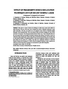
One can see that an additional third term is added to the original constraint function which perturbs the original constraint. Here ε > 0 is a small relaxation parameter which controls the amount of relaxation and (ρ − 1) serves to avoid introducing relaxation for solid material. Note that in this formulation no singular optima exists. Since for any ε > 0 Equation (6) will be satisfied when ρ is sufficiently small [12]. Equation (6) is thus always satisfied in the vicinity of ρ = 0. Another alternative relaxation technique is the qp-approach [13] in which the relaxed stress constraint is defined as: khσ0 ik − 1 ≤ 0, where q < p. (7) gqp = ρp−q σlim In this case, q is not chosen equal to p to be consistent with microstructural considerations. Instead, it is taken as q < p to relax the constraint by imposing zero stress for zero density. Equation (7) is also always satisfied for any q < p and a sufficiently small ρ. In general, the relaxed stress constraint can be written as: khσ0 ik ≤ ϕ(ε, ρ), (8) σlim where ϕ represent the relaxed normalized stress limit as a function of the design variable ρ and the relaxation parameter ε, for the formulations adopted in ε-relaxation for density-based optimization [19] and the qp-approach [13], respectively. For the qp-approach we define this relaxation parameter as εqp = p−q (note that ε and εqp are not directly comparable in terms of the resulting degree of relaxation). The behaviour of ϕ as a function of the density and for different values of the relaxation parameters is shown in Figure 1. To do a fair comparison, we have chosen εqp in such a way, that the same degree of relaxation is obtained at a lower density ρmin = 1e−3, as for ε-relaxation (for a given ε). The trend of the curves is similar for ε-relaxation and the qp-approach and it can be seen that in both cases, activation of stress constraints at low densities is avoided by increasing the feasible stress limit. However, as pointed out in [13], the qp-approach does not introduce a perturbation only in proximity of the singularity zone, but on a larger range of densities. The ε-relaxation approach approximates more the original stress over the density range and only perturbs it in the vicinity of ρ = 0. This has an influence on the convergence properties of the relaxed problem. Both relaxation techniques circumvent the problems of singular optima since the design space does not contain any degenerate subspaces and therefore the optima are in principle accessible by any gradientbased solution technique. Unfortunately, the relaxed design space is highly non-convex and therefore prone to convergence to local optima.

4

5

5

ϕ

ϕ ϕ = 1 + ε/ρ − ε

4

ϕ = 1 + ε/ρ − ε

4

ϕ = ρq-p

ϕ = ρq-p

3

3

2

2

1

1

0 0

0.2

0.4

0.6

0.8

ρ

0 0

1

0.2

(a) ε = 0.1, εqp = p − q = 0.67

0.4

0.6

0.8

ρ

1

(b) ε = 0.001, εqp = p − q = 0.10

Figure 1: Variation of the parameter ϕ with the density for the ε-relaxation approach [19] in density-based optimization and the qp-approach [13] and different values of the relaxation parameters. 3

Numerical tests and discussion

In this section, we present an elementary numerical example on which we study effect of penalization and stress relaxation using the qp-approach, on the existence and accessibility of (local) optima. Furthermore, we consider the effect of mesh refinement and aggregation. h

End state

h=1

h = 1/2

1

h

3 1 h

*

2 10 h=0

Initial State

(a) Two member structure for position h∗ = 1/2

Region in which we consider the Von Mises Stress in each element

(b) The member moves through the fixed finite element mesh (10×3) used for our base-example. The numerical representation for the middle position of the member is shown in Figure 3

Figure 2: Example of a structure build up of two horizontal members of which the upper member is allowed to move continuously in the vertical direction by amount h ∈ [0, 1]. For the sake of clarity, the begin- (h = 0), middle- (h = 1/2) and end position (h = 1) are shown. The example we consider is the structure depicted in Figure 2(a), which consists of two horizontal members clamped on the left end and subjected to a distributed load on the right end. The upper horizontal member is allowed to vary continuously in vertical direction by amount h ∈ [0, 1] and is

5

depicted for position h∗ = 1/2. For the sake of clarity, in Figure 2(b) three positions for the member are shown on the fixed finite element discretization. The member is restricted to preserve its rectangular shape and size (the amount of material is constant). Thus, it is important to note that we are not considering a topology optimization problem in which the each density is treated as a design variable. In our problem there is only one design variable, h, which is the position of the upper horizontal member. However, our example serves to study situations that may occur in density-based topology optimization. Similar as in most density-based topology optimization problems we work with a fixed design domain which is modeled by a fixed finite element discretization. The design is parameterized by assigning density variables to each finite element which can vary continuously between zero and one, representing void and solid material, respectively. The material properties of each finite element are then parameterized as in Equation (2). Thus, the member moves through the mesh as can be seen in Figure 2(b). In Figure 3 the numerical presentation of the member positioned at h = 1/2, is shown.

Figure 3: The position of the beam element (left) and its numerical representation by intermediate densities (right) The following questions arise: how does the stress response behave with respect to the position of the horizontal member? How will the different measures (penalization, stress relaxation) and discretization influence this behaviour? Here, we will consider the Von Mises stress in the n elements that lie in the region inside the red box in Figure 2(b): these are stored in the vector σvm = [σvm,e ] for e = 1..n. These elements will experience the largest deformation; high stresses that might occur around the corners at both ends of the horizontal member are neglected. For this example we state our optimization problem as follows: finding the minimum of the maximum Von Mises stress subjected to a volume constraint. This is formulated as: min S = max (σvm )

h∈[0,1]

s.t. V ≤ Vlim ,

(9)

where S is the objective function, which is the maximum Von Mises stress for elements we consider, in position h. V and Vlim are the volume and volume limit, respectively. The design variable and its design domain are denoted as h ∈ [0, 1]. For a single element e the relaxed Von Mises stress is formulated as: σvm,e = ρep−q σvm,0 , where q ≤ p,

(10)

where σvm,0 is the Von Mises stress assuming solid material properties. Note that this formulation in Equation (10) represents both, the relaxed and unrelaxed stress, depending on the choice of q. When we apply the qp-approach for stress relaxation, then q < p, and otherwise q = p. For this example problem, when the void would not be modeled, the lowest stresses are obtained for the configuration h = 1. This corresponds to the global, physically optimal solution. In the considered fixed-mesh setting, however, we may need to relax the stress responses due to the presence of the singularity phenomenon. Furthermore, unlike the real physics where the axial- and bending stiffness of the moving member does not depend on its position, in the numerical model it does. It was already shown by van Dijk et al. [17] on a similar example for the compliance case, that ‘artificial’ local optima could arise due to the design parameterization and/or discretization. Thus, we are interested to investigate whether this also occurs in case of the stress response, and how it affects the accessibility of the global optimum. This example is chosen since it may represent a situation in topology optimization that a member converges to a local optimum, but a small movement of that member may lead to a more optimal design. The nature of the stress response prevents this from happening. Furthermore, the effect of penalization will be particularly noticeable in this example due to the contribution of intermediate densities to the bending and tensional stiffness of the member. Since the stiffness of intermediate density elements becomes relatively low when penalization is performed, the overall bending of the structure will thus temporarily increase, when moving the member vertically in h-direction, before reaching the optimal 6

state. Therefore, to reach the optimum in h = 1, one would have to pass an extremely unfavourable condition. It is thus of interest how the stress responses behave for intermediate densities and how this can be related to the penalization exponent for the design parameterization and applied stress relaxation. Note that the beam is restricted to preserve its rectangular shape and therefore changes only occur at its boundary. In that sense it differs from density-based topology optimization in which the material is allowed to change element-wise. However, this example may represent situations in density-based topology optimization in which the solution is close to convergence and changes that occur, are mainly along the structural boundary, while the volume constraint remains active. First, we study the effect of qp-relaxation on the behavior of the stress response, without and with penalization. Then, the global trajectories are discussed when relaxation is applied in a continuation strategy. Finally, we study the effect of a relative mesh refinement for the same problem. In the figures we use different letters to refer to particular response function values in the design domain h ∈ [0, 1]. For example, A is a response function value which location is denoted as hA . Furthermore, if at this location the objective function takes the value of A (i.e. A is the maximum stress value at that location), we refer to it as SA . For all examples the structure is modeled assuming plane-stress and for the finite element computation, four-noded bilinear isoparametric quadrilaterals are used. Poisson’s ratio is ν = 0.3 and the Young’s modulus is E = 1. The mesh of our base-example is 10 × 3 elements. 3.1

Effect of qp-relaxation on the stress response without penalization

First, let us consider the case in which no penalization and no relaxation is applied, i.e. p = 1 and εqp = p − q = 0 in Equation (10), respectively. In Figure 4 the Von Mises stresses are plotted as a function of the position h of the moving member.

σvm

σ1

E

σ2

h 2

σ3

D 1.5

1

A C

0.5

B 0 0

0.1

0.2

0.3

0.4

0.5

0.6

0.7

0.8

0.9

h

1

Figure 4: No penalization (p = 1) and no relaxation (εqp = 0): the Von Mises stress for the three elements in the middle column as a function of the position h of upper horizontal member Note that the objective function S is the maximum stress for each position h. The first observation is that the global and only optimum of this numerical problem is located at hC and not at the true physical optimum, h = 1. Thus, SC can be regarded as an artificial optimum which is related to the singularity phenomenon. This can be observed by noting that the maximum stress values in both begin and end position are overestimated and correspond to void elements. Thus, in the begin position, the objective function is SD which corresponds to the stress of the upper element σvm3 (0), which is void in that position. Physically, the objective function in the begin position should be SA , which correspond to the stress in the middle element σvm2 (0). In the end position the same problem arises where SE , which correspond to the stress of the middle element which is void. Therefore, the true physical optimum B at h = 1 cannot be reached by a typical gradient-based optimization algorithm. Thus, A and B are singular optima.

7

Next, we relax the stress responses following the qp-approach, i.e. q < p in Equation (10). The result is shown in Figure 5 for εqp = p − q = 0.2. It can be observed that the singular optima A and B, for the problem without relaxation, are now indeed the correct values for the maximum stress S for the begin and end state. Which solves the problem, with respect to the presence of the singularity phenomenon. However, there is still a local optimum SC 0 stress which can be regarded an artificial as SC in the unrelaxed example in Figure 4. Thus, stress relaxation eliminates the singularity phenomenon, but the relaxed problem still contains artificial optima. In general, a continuation strategy is applied to solve this problem, in which the degree of relaxation is gradually decreased, i.e. εqp → 0. However, it will be shown in Section 3.3 that this does not converge to the true physical optimum, h = 1.

σvm

σ1

1

σ2

h

A

σ3

C’

0.8

0.6

B 0.4

0.2

0 0

0.1

0.2

0.3

0.4

0.5

0.6

0.7

0.8

0.9

1

h Figure 5: No penalization (p = 1) with relaxation (εqp = 0.2): the Von Mises stress for the three elements in the middle column as a function of the position h of upper horizontal member 3.2

Effect of qp-relaxation on the stress response with penalization

The same numerical example is considered but now with penalization (the usual value used in densitybased topology optimization in 2-D is used, p = 3). The results are shown in Figure 6, where Figure 6(a) are the stress responses without relaxation and in Figure 6(b) the relaxed stress responses, εqp = 0.2. As expected, in both cases (no relaxation vs. relaxation) the stress values for h = 0 and h = 1 are equal as in the case without penalization Figure 4, since in these positions the structure is represented entirely by solid elements and penalization and relaxation only have effect on the effective material properties and stress model for intermediate density elements. Thus, again, as in the case without penalization the problem is subjected to the singularity phenomenon and the maximum stress in begin and end position is overestimated by stress values corresponding to void elements. The effect of penalization on the stress response can be seen for all 0 < h < 1 where the member is represented by intermediate density elements. It can be seen that the stress values for these elements have become relatively high, making them unfavourable in terms of stress minimization and thus promoting a 0-1 design. In the relaxed case in Figure 6(b) the singular stress values SA and SB are now the correct objective function values in begin and end position. Thus, the true physical optimum SB is now accessible. However, it can be seen in Figure 6(b) that penalization also lead to a higher degree of non-convexity of the stress responses and SA is now introduced as a local optima. For every initial position 0 ≤ h ≤ 0.4, a gradient-based optimizer will converge to the local optimum SA . Finally, note that there is still an optimum with intermediate density elements, SC 0 , despite the applied penalization. For the right amount of stress relaxation and applying a continuation strategy, it may be possible to avoid convergence to such local optima. Next, wel will consider the qp-relaxation in a continuation strategy.

8

3.5

3.5 σ1

σvm

2

3

σ1

σvm

σ

σ2

3

σ

σ3

3

2.5

2.5

E 2

2

D 1.5

1.5

A

1

C

A

1

C’

B 0.5

0.5

0 0

0.1

0.2

0.3

0.4

0.5

0.6

0.7

0.8

0.9

B

0

1

0

h

0.1

0.2

(a) p = 3, εqp = 0

0.3

0.4

0.5

0.6

0.7

0.8

0.9

h

1

(b) p = 3, εqp = 0.2

Figure 6: The stress responses as a function of the position h of the upper horizontal member 3.3

Continuity of the global trajectory

In general, constraint relaxation is applied in a continuation strategy, i.e. the original problem is relaxed and the amount of relaxation is gradually decreased towards the original optimization problem. However, for the ε-relaxation technique [12] it was shown by Stolpe and Svanberg [16] on a truss optimization example, that the global trajectories may be discontinuous. Here the global trajectory is defined as the path followed by the global solution to the relaxed problem in a continuation strategy. The same was shown for the qp-approach by Bruggi [13]. Thus, this implies that the global optimum of the relaxed problem (ε-relaxation and qp-approach) may not converge to the global optimum of the original problem in truss optimization. In this section, we show an extension of these results to our continuum structure in Figure 2, in which the design is parameterized as in density-based topology optimization. Next, we will apply relaxation in a continuation strategy on our two member example shown in Figure 2 and we plot the Von Mises stress responses for the three considered elements. The penalization exponent is now chosen as p = 1.2 and the stress is relaxed by the qp-approach, gradually decreasing the relaxation parameter, εqp = 0.8 → 0.1. It will be shown that, in agreement with the results obtained in truss optimization, the global trajectory for our example in density-based topology optimization, may be discontinuous. 1.4

1.4

Xvm

σ1 σ2

h

1.2

σvm

σ1 σ2

1.2

σ3

σ3

1

1

A

A 0.8

0.8

0.6

0.6

B

B

0.4

0.4

C

C

0.2

0.2

0

0

0

0.1

0.2

0.3

0.4

0.5

0.6

0.7

0.8

0.9

h 1

0

(a) Sequence of solutions of the relaxed problem during continuation

0.1

0.2

0.3

0.4

0.5

0.6

0.7

0.8

0.9

h 1

(b) Global trajectory

Figure 7: Von Mises stress relaxation by qp-approach in a continuation strategy. Penalization factor is p = 1.2 and relaxation parameter is varied over εqp = 0.8 → 0.1 The dotted lines are the Von Mises stress responses for the initial relaxed problem (εqp = 0.8 and the solid lines are the responses after relaxation εqp = 0.1). 9

In Figure 7, the dotted lines represent the stress responses for the initial relaxation εqp = 0.8, from which we start our continuation strategy and the solid lines represent the stress responses at the end of the continuation strategy εqp = 0.1. In Figure 7(a) we consider the sequence of solutions to the relaxed problem and in Figure 7(b) the path followed by the global optimum is considered. It can be seen that for the initial state of relaxation, SC is the global optimum. The sequence of solutions to the relaxed problem following a continuation approach is represented by the blue asterixes. It can be seen that the initial global optimum SC converges to the local optimum in SA when following a continuation approach and not the global optimum SB of the original problem. Therefore, the global trajectory is discontinuous for the relaxation problem. This can be seen clearly in Figure 7(b), where the trajectory of global solutions is represented by the red asterixes and the large arrow indicates the sudden jump for a certain εqp . A more illustrative figure of this problem is shown in Figure 8 where the locations of the optima in the design domain h ∈ [0, 1] are plotted versus the relaxation parameter εqp . Here the trajectories are displayed in the h − εqp plane. The blue line is the solution path of the relaxed problem and the red line represents the global trajectory. It can be seen that, despite the fact that the initial solution is on the global trajectory, there exists an εqp for which the global trajectory is discontinuous. In the figure, the large arrow indicates the sudden jump for εqp = 0.63, where the global solution is located at hB while the solution for decreasing εqp while converges towards the local optimum at hA . Similar results were obtained by us, using the ε-relaxation approach in a continuation strategy for our problem. Furthermore, both results where validated analytically on a truss-based optimization example. It can thus be concluded that, in agreement with the results obtained in truss optimization [13, 16], the global trajectory may be discontinuous, i.e. the sequence of solutions to the relaxed problem may not converge to the global optimum of the original problem. This can even be the case for problems where the initial point is on the global trajectory as for our problem.

1

εqp 0.9

(hC,0.8)

0.8 0.7

εqp = 0.63

0.6 0.5 0.4 0.3 0.2 0.1 0

(hA,0.1) 0

0.1

(hB,0.1) 0.2

0.3

0.4

0.5

0.6

0.7

0.8

0.9

h

1

Figure 8: The optima plotted in the (h-εqp )-plane. The blue line is the sequence of solutions for relaxed problem and the red line is the global trajectory. 3.4

Mesh refinement

In our elementary numerical example in Figure 2, a coarse mesh was used in which the thickness is equal to the height of a finite element. Therefore, the difficulties introduced by the introduction of intermediate density elements, might be more noticeable in our optimization problem than for the same case with a finer mesh, since these elements form a relatively large part of the whole structure when using a coarse mesh. In this section, we will investigate the effect of a relative mesh refinement, using the same example considering penalization and stress relaxation following the qp-approach. For the sake of simplicity, we choose a fixed relaxation parameter. Furthermore, we consider a relative mesh refinement of 3, shown in Figure 9.

10

Region in which we consider the Von Mises Stress in each element

h

Figure 9: Two member problem of Figure 2 with relative mesh refinement of 3. Mesh is 30 × 9. Note that in this figure the member is positioned at h = 1/3. Here, we consider the the Von Mises stress for the elements in the region inside the red box in Figure 9. The structural problem is the same as before: the upper member can vary its position h ∈ [0, 1]. Note that now there are four positions in which the upper horizontal member coincides exactly with the finite element mesh: h = 0, h = 1/3, h = 2/3 and h = 1. At these positions, only solid and void elements exist and no intermediate density elements are present. In our previous example with the coarse mesh, this was only the case at begin and end position. First, we consider the problem without penalization, p = 1. The results are shown in Figure 10, where we consider both cases, with and without stress relaxation. In Figure 10(a), the stress responses are shown for the case without relaxation. It can be seen, that high peak stresses occur around the positions mentioned above where the position of the member coincides with the mesh. This is the same effect we observed for a coarse mesh (Figure 4) and caused by the presence of the singularity phenomenon. In h = 0, the maximum stress corresponds with the stress of the upper element which is void. Furthermore, in the other positions jumps in the stress response can be observed, which are caused by that particular element becoming void. Again, as in our original problem with the coarse mesh, a typical gradient-based optimizer would not be able to reach the global optimum in h = 1. When we apply qp-relaxation, with a relaxation parameter of εqp = 0.2, the resulting stresses are depicted in Figure 10(b). It can be seen that there are now three optima, including the global optimum of the original problem. In the figure the corresponding configuration of the structural member is shown for these optima. It can be seen that the local optima correspond to configuration of the structure in which boundary of the member is represented by intermediate density elements. Xvm

σvm 3

3

2.5

2.5

2

2

1.5

1.5

1

1

0.5

0.5

h=0.17 h

h=0.54

h=1

0

0 0

1/6

2/6

3/6

4/6

5/6

h

1

0

(a) No penalization (p = 1) and no relaxation (εqp = 0)

0.1

0.2

0.3

0.4

0.5

0.6

0.7

0.8

0.9

h

1

(b) No penalization (p = 1) with relaxation (εqp = 0.2)

Figure 10: Relative mesh refinement: 30 × 9. The Von Mises stress is plotted for the elements the middle column as a function of the vertical position h of the moving member. . Now, let us consider the problem with penalization (p = 3), as applied in density-based topology optimization. In Figure 11 it can be seen what effect this has on the stress responses. From Figure 11(a) 11

it is clear that high peak stresses occur at the same location as in the case without penalization, which is obvious since penalization only has effect on intermediate density elements. Thus, the difference are the higher stress values for intermediate density elements, which is effectively the desired effect of penalization: making intermediate density elements unfavourable in terms of stress. However, the side effect is that this increases the degree of non-convexity of the stress response. Next, we consider the case with penalization and relaxation as considered in density-based optimization. The effect of qp-relaxation with a relaxation parameter of εqp = 0.2, can be seen in Figure 11(b). Note that there are no singular optima and the global optimum is accessible. The effect of penalization can be seen best by comparing the relaxed cases Figure 10(b) and Figure 11(b), it can be seen that the optima for the case with penalization are found for positions of the member where no intermediate densities are present, whereas when no penalization is applied, these local optima are generally found for solutions with intermediate densities. Another observations is that the degree of non-convexity is higher with penalization. Note, that there is one local optimum in which intermediate densities are present (hC ≈ 0.13), this is due to the qp-relaxation and will disappear for εqp → 0. 3.5

3.5

σvm

h=1/3

Xvm

3

3

h

h=2/3 2.5

2.

2

2

1.5

1.5

h=1 C 1

1

0.5

0.5

0

0 0

1/6

2/6

3/6

4/6

5/6

h

1

0

(a) Penalization (p = 3) and no relaxation (εqp = 0)

0.1

0.2

0.3

0.4

0.5

0.6

0.7

0.8

0.9

h

1

(b) Penalization (p = 3) with relaxation (εqp = 0.2)

Figure 11: Relative mesh refinement: 30 × 9. The Von Mises stress is plotted for the elements inside the red box, as a function of the vertical position h of the moving member. . Finally, the example is considered for a mesh refinement of six times the original mesh. Since it is clear that problems of singular optima are not improved by mesh refinement we will here immediately consider the relaxed stresses. Furthermore, we plot an aggregated stress function (P-Norm for P = 12) which is often used when dealing with a large number of constraints. The results are shown in Figure 12. Note that the high peak stress in Figure 12(b) confirms the observation that mesh refinement does not improve the results with respect to the singularity phenomenon.

12

3.5

3.5

σvm

σvm

3

3

P-Norm Stress (P=12)

P-Norm Stress (P=12) 2.5

2.5

2

2

1.5

1.5

1

1

0.5

0.5

0

0 0

1/6

2/6

3/6

4/6

5/6

h

1

0

(a) No penalization (p = 1) with relaxation (εqp = 0.2)

1/6

2/6

3/6

4/6

5/6

h

1

(b) Penalization (p = 3) with relaxation (εqp = 0.2)

Figure 12: Relative mesh refinement: 60×18. The Von Mises stress is plotted for the elements the middle column as a function of the vertical position h of the moving member. The line on top, is the aggregated P-Norm stress for P = 12. . It can be concluded, that mesh refinement did not change the nature of the problem with respect to the presence of singular optima. However, it can be observed that mesh refinement decreases the degree of non-convexity of the stress response and the objective function becomes smoother. This is particularly noticeable for the case with penalization by comparing the coarse mesh in Figure 6(b) and the fine mesh in Figure 11(b). The amplitude of the wiggles for intermediate densities becomes less. Finally, it can be observed that the aggregated stress function also has a smoothing effect. One final note is that in our example the best results are obtained for the case without penalization since the behavior of the response function is smoother between the begin and end state. However, note that in our example the member is artificially restricted to preserve its shape and size which is not the case in density-based topology optimization, where penalization is needed to promote a 0-1 design. 4

Conclusions and future work

Topology optimization including stress constraints is known to be a difficult problem, and application of existing techniques often leads to convergence to local (artificial) optima. In order to gain a better understanding of the underlying reasons for these difficulties, a numerical study has been performed. The presented numerical inverstigation of stress responses in a 2-D SIMP continuum topology optimization setting leads us to the following conclusions with regard to singular optima and relaxation: 1) The singularity phenomenon, i.e. the existence of inaccessible optimal solutions known from truss sizing problems, has also been observed and confirmed in a 2-D continuum example. Therefore, clearly, relaxation techniques are necessary in the presented formulation. 2) It has been confirmed that relaxation techniques, such as the studied ε-relaxation and qp-approach, solve the singularity problem and make the global optimum accessible. 3) However, as observed earlier by truss-based studies [13, 16], also for the 2-D continuum case we observe that relaxation and continuation can easily converge to a local optimum. In addition, regarding penalization, the numerical results show that increasing degrees of penalization lead to an increasing degree of non-convexity of the stress response. Convergence to inferior local optima therefore is expected to become more likely as penalization is increased. Finally, increasing the relative mesh refinement (number of finite elements per minimum member size) was found to diminish the degree of non-convexity of the stress response, and constraint aggregation in addition had a further smoothing effect. Based on these observations, it appears attractive to (initially) avoid the use of strong penalization, to use a fine mesh relative to the minimum member size, and to exploit the smoothing effect induced by constraint aggregation. But avoiding the presence of intermediate densities along the boundary altogether (in e.g. a level set-based approach, in combination with partition-of-unity methods) could be an effective alternative way to avoid the mentioned convergence problems.

13

References [1] M.P. Bendsøe. Optimal shape design as a material distribution problem. Structural and multidisciplinary optimization, 1(4):193–202, 1989. [2] M.P. Bendsøe and O. Sigmund. Topology optimization: theory, methods, and applications. Springer Verlag, 2003. [3] G. Sved and Z. Ginos. Structural optimization under multiple loading. International Journal of Mechanical Sciences, 10(10):803805, 1968. [4] U. Kirsch. Optimal topologies of truss structures 1. Computer Methods in Applied Mechanics and Engineering, 72(1):1528, 1989. [5] U. Kirsch. On singular topologies in optimum structural design. Structural and Multidisciplinary Optimization, 2(3):133–142, 1990. [6] G.I.N. Rozvany and T. Birker. On singular topologies in exact layout optimization. Structural and Multidisciplinary Optimization, 8(4):228235, 1994. [7] G.I.N. Rozvany. Difficulties in truss topology optimization with stress, local buckling and system stability constraints. Structural and Multidisciplinary Optimization, 11(3):213–217, juni 1996. [8] G.I.N. Rozvany. On design-dependent constraints and singular topologies. Structural and Multidisciplinary Optimization, 21(2):164–172, april 2001. [9] R. J. Yang and C. J. Chen. Stress-based topology optimization. Structural and Multidisciplinary Optimization, 12(2):98–105, 1996. [10] J. Par´ıs, F. Navarrina, I. Colominas, and M. Casteleiro. Improvements in the treatment of stress constraints in structural topology optimization problems. Journal of computational and applied mathematics, 234(7):2231–2238, 2010. [11] P. Duysinx and M.P. Bendsøe. Topology optimization of continuum structures with local stress constraints. International Journal for Numerical Methods in Engineering, 43(8):1453–1478, 1998. [12] G.D. Cheng and X. Guo. ε-relaxed approach in structural topology optimization. Structural and Multidisciplinary Optimization, 13(4):258–266, 1997. [13] M. Bruggi. On an alternative approach to stress constraints relaxation in topology optimization. Structural and Multidisciplinary Optimization, 36(2):125–141, 2008. [14] M. Koˇcvara and J.V. Outrata. Effective reformulations of the truss topology design problem. Optimization and Engineering, 7(2):201–219, 2006. [15] C. Le, J. Norato, T. Bruns, C. Ha, and D. Tortorelli. Stress-based topology optimization for continua. Structural and Multidisciplinary Optimization, 41(4):605–620, 2010. [16] M. Stolpe and K. Svanberg. On the trajectories of the epsilon-relaxation approach for stressconstrained truss topology optimization. Structural and Multidisciplinary Optimization, 21(2):140– 151, april 2001. [17] N.P. van Dijk, M. Langelaar, and F. van Keulen. Critical study of design parameterization in topology optimization; The influence of design parameterization on local minima. In Proceedings of the 2nd International Conference on Engineering Optimization, 2010. [18] O. Sigmund. Morphology-based black and white filters for topology optimization. Structural and Multidisciplinary Optimization, 33(4):401–424, 2007. [19] P. Duysinx and O. Sigmund. New developments in handling stress constraints in optimal material distributions, 1998.

14