Effect of nonlinear dispersion on pulse self-compression in a

Physica D 240 (2011) 963–970

Contents lists available at ScienceDirect

Physica D journal homepage: www.elsevier.com/locate/physd

Effect of nonlinear dispersion on pulse self-compression in a defocusing noble gas Christian Köhler a,∗ , Luc Bergé b , Stefan Skupin a,c a

Max Planck Institute for the Physics of Complex Systems, 01187 Dresden, Germany

b

CEA-DAM, DIF, F-91297 Arpajon, France

c

Friedrich Schiller University, Institute of Condensed Matter Theory and Optics, 07743 Jena, Germany

article

info

Article history: Received 30 September 2010 Accepted 5 February 2011 Available online 15 February 2011 Communicated by S. Kai Keywords: Ultrashort pulse compression Modulational instability Spatio-temporal dynamics Kerr nonlinearity Dispersive nonlinearity Nonlinear Schrödinger equation

abstract Media with a negative Kerr index (n2 ) offer an intriguing possibility to self-compress ultrashort laser pulses without the risk of spatial wave collapse. However, in the relevant frequency regions, the negative nonlinearity turns out to be highly dispersive as well. Here, we study the influence of nonlinear dispersion on the pulse self-compression in a defocusing xenon gas. Purely temporal (1 + 1)-dimensional investigations reveal and fully spatio-temporal simulations confirm that a temporal shift of high intensity zones of the compressed pulse due to the nonlinear dispersion is the main effect on the modulational instability (MI) mediated compression mechanism. In the special case of vanishing n2 for the center frequency, pulse compression leading to the ejection of a soliton is examined, which cannot be explained by MI. © 2011 Elsevier B.V. All rights reserved.

1. Introduction The common property of laser pulse compression schemes is the utilization of nonlinear effects the pulse undergoes upon propagation. The omnipresent idea hereby is to broaden the pulse spectrum and ensure a flat spectral phase at the same time. Among others, such as frequency conversion in filaments [1] or cascading quadratic nonlinearities [2–4], the spectral broadening ability of self-phase modulation (SPM) is often exploited in the guided configuration (waveguides, fibers). The resulting phase can be accounted for by applying some post-compression mechanisms such as Bragg gratings and chirped mirrors or, even more convenient, by a counteracting term on the phase contributions, that is in our case the group velocity dispersion (GVD). The simplest model that captures both processes is expressed by the famous nonlinear Schrödinger (NLS) equation for the slowly varying envelope of an optical pulse A(z , t ) : ∂z A = −ik2 Att /2 + iγ |A|2 A. Here, k2 = ∂ 2 k(ω)/∂ω2 |ω=ω0 is the GVD coefficient at center frequency ω0 and γ = n2 ω0 /c is the Kerr coefficient with index n2 ∝ χ (3) defined by the third order susceptibility tensor χ (3) . The standard case described above would be anomalous GVD (k2 < 0) counteracting on positive Kerr response (γ > 0), since a negative second derivative of the wave number k2 is

more common than a negative γ . Trying to transfer this ’’solitary compression mechanism’’ to the unguided bulk setup gives rise to problems due to self-focusing and subsequent collapse of the beam in the transverse spatial directions. Resolving this problem and still sticking to the ’’solitary compression’’ (phase cancelation due to different signs of GVD k2 and SPM γ ) means to ensure a negative γ . Indeed, negative values for the Kerr response can be found, e.g., in the UV near two photon resonances in Xe (Ref. [5]). However, the strong dispersion of the nonlinearity near these resonances questions the compression mechanism which is based on a constant nonlinearity. Nevertheless, it was shown recently [6] and will be elucidated in more detail in this work, that the basic compression mechanism survives these obstacles. Moreover, we will present an alternative scenario where pulse compression is actually caused by the nonlinear dispersion, while the Kerr index n2 approaches zero at center wavelength. The paper is organized as follows. In Section 2, we give a short derivation of our wave equation, followed by a discussion of the temporal dynamics in a (1 + 1)-dimensional configuration in Section 3. Finally, in Section 4, results for the (3 + 1)dimensional setup with radial symmetry are presented and discussed. Conclusions are drawn in the last section. 2. Derivation of the governing equation 2.1. From Maxwell’s to wave equations

∗

Corresponding author. Tel.: +49 3518712213; fax: +49 3518711999. E-mail address: [email protected] (C. Köhler).

0167-2789/$ – see front matter © 2011 Elsevier B.V. All rights reserved. doi:10.1016/j.physd.2011.02.004

The propagation of light through a (nonlinear) optical medium is described by the macroscopic Maxwell’s equations. We assume

964

C. Köhler et al. / Physica D 240 (2011) 963–970

the absence of free charges ρf = 0 and free currents J⃗f = 0, a

⃗ = µ0 H ⃗ and the material to be nonlinear in nonmagnetic medium B ⃗ ⃗ ⃗ the sense that D = ϵ0 E +P. It is common to express the polarization ⃗ P⃗ = P⃗ (1) + P⃗ (3) + P⃗ (5) + · · · , P⃗ (j) ∼ E⃗ j , P⃗ in a power series in E: where we already accounted for the vanishing of contributions of even power in E⃗ because we are dealing with centrosymmetric media. In this work, we keep only terms up to third order and refer to P⃗ (1) = P⃗L as the linear polarization and to P⃗ (3) = P⃗NL as the nonlinear part. Putting all together, we get a wave equation in a form that is often used as starting point for further calculations ∂ 2 E⃗ ∂ 2 P⃗L ∂ 2 P⃗NL ∇ E⃗ = µ0 ϵ0 2 + µ0 2 + µ0 + ∇(∇ · E⃗ ). (1) ∂t ∂t ∂t2 ⃗ · E⃗ is negligible. Furthermore, For small polarization |P⃗ | ≪ |ϵ0 E⃗ |, ∇ 2

we restrict our analysis to linearly polarized light and disregard the tensor nature of the material response. Together with the paraxiality assumption, we can omit vector arrows and treat a scalar equation for the dominating field component. In Fourier space, the linear polarization can be expressed as P˜ L (ω) = ϵ0 χ (1) (ω)E˜ (ω) and after introducing the wave number k(ω) = 1 + χ (1) (ω)ω/c we obtain the wave equation in Fourier space

∇ 2 E˜ + k2 (ω)E˜ = −ω2 µ0 P˜NL .

(2)

In this work, we focus on the description of forward propagating waves only, since backscattered waves as well as the coupling between both directions are usually weak for our beam configurations [7]. We assume the field to propagate mainly along the z ≥ 0 direction and therefore decompose it into forward propagating plane waves with wave numbers k(ω) and the envelope A˜

∫

dωA˜ (x, y, z , ω)ei[k(ω)z −ωt ] .

(3)

2 Distinction of the directions by ∇ 2 = ∇⊥ + ∂z2 allows us to neglect the fast varying backward traveling part of A by skipping terms ∼∂z2 as long as the slowly varying envelope condition |∂z2 | ≪ |2ik(ω)∂z | holds for the forward propagating part. Then, in Fourier space the so-called forward Maxwell equation [8] emerges naturally

∂z A˜ =

i 2k(ω)

i µ0 ω ∇⊥2 A˜ + ik(ω)A˜ + P˜ NL . 2k(ω) 2

(4)

Eq. (4) is in principle valid in the whole spectral domain. However, in this work, our radiation is limited to a finite frequency window around the laser operating frequency ω0 . Hence, it is useful to Taylorize the dispersion relation k(ω) = k0 +

k1 1!

ω¯ +

k2 2!

ω¯ 2 + · · · ,

(5)

with kj = ∂ j k(ω)/∂ωj |ω=ω0 and ω ¯ = ω − ω0 . Moreover, for convenience in the numerics, we split fast oscillations in z and go over to a co-moving time frame, defined by t → t + k1 z. In Fourier space, this leads to the introduction of the (normalized) slowly varying complex envelope 1

¯ z E˜ (ω) ¯ = Θ (ω¯ + ω0 ) √ E˜ (ω¯ + ω0 )e−i(k0 +k1 ω) ,

s

s=

P˜ NL (ω) = ϵ0 s3/2

∫∫

dω1 dω2 χ (3) (−ω; ω − ω1 − ω2 , ω2 , ω1 )

¯ z × 3E˜ (ω¯ 1 )E˜ (ω¯ 2 )E˜ ∗ (ω¯ 1 + ω¯ 2 − ω) ¯ ei(k0 +k1 ω) ,

(7)

where * means complex conjugate. With this expression, we can finally write down the propagation equation for the slowly varying complex envelope

∂z E˜ =

i

∇⊥2 E˜ + i[k(ω) − k0 − k1 ω] ¯ E˜ ∫∫ 3iω2 s + dω1 dω2 χ (3) (−ω; ω − ω1 − ω2 , ω2 , ω1 ) 2k(ω)c 2 2k(ω)

× E˜ (ω¯ 1 )E˜ (ω¯ 2 )E˜ ∗ (ω¯ 1 + ω¯ 2 − ω). ¯

(8)

In the following analysis, we take the linear dispersion for Xe from Ref. [9] and the nonlinear dispersion χ (3) is given in Ref. [10]. 3. (1 + 1)-dimensional setup

2.2. Forward propagating equation for the complex field

E (x, y, z , t ) =

we are only interested in contributions having approximately the same frequency ω0 as our initial pulse and therefore omit terms responsible for higher order harmonics generation. Hence, the resulting expression for a dispersive third order nonlinear polarization in Fourier domain is

1 2n0 ϵ0 c

, (6)

with |E |2 = I being the laser intensity, Θ (x) the usual Heaviside function, and n0 = k0 c /ω0 . 2.3. Including the nonlinearity As for the linear polarization, the tensor nature of the nonlinear response function χ (3) is neglected. Furthermore,

In a first approach we want to investigate purely temporal influence of the dispersive nonlinearity on pulse dynamics, thus 2 skipping the transverse spatial derivatives (∇⊥ ) in Eq. (8). Even if the numerical solution of this equation is straightforward, it does not elucidate the underlying mechanisms for compression. In order to get some deeper insight, we include subsequently increasing orders of nonlinear dispersion, originating from a Taylor expansion around the central frequency ω0 :

χ (3) (−ω; ω − ω1 − ω2 , ω2 , ω1 ) = χ0(3) + χ1(3) ω¯ 1 + χ2(3) ω¯ 2 + χ3(3) ω¯ + · · · ,

(9)

where ω ¯ j = ωj − ω0 and

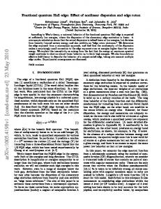
χ0(3) = χ (3) (−ω0 ; −ω0 , ω0 , ω0 ), χ1(,32) = ∂ω1,2 χ (3) (−ω; ω − ω1 − ω2 , ω2 , ω1 )|ω1 =ω2 =ω=ω0 , χ3(3) = ∂ω χ (3) (−ω; ω − ω1 − ω2 , ω2 , ω1 )|ω1 =ω2 =ω=ω0 . By doing so, we are able to attribute specific effects to the corresponding orders of nonlinear dispersion. In a first step, we (3) neglect nonlinear dispersion (χ1,2,3 = 0) and explain the basic mechanisms of compression occurring in this case. In a second step, first order terms of nonlinear dispersion are included and their influence upon compression is investigated. Finally, the results are compared with the ones obtained from the fully dispersive (1 + 1)dimensional model. As mentioned above, we are interested in setups with negative n2 ∼ χ (3) , which can be found near resonances in Xe [see Fig. 1]. So for the coming simulations, we introduce the abbreviation ω−− = 7.73 × 1015 s−1 for the characteristic central frequency ensuring a negative n2 and additionally ω00 = 7.91 × 10−15 s−1 for investigations with vanishing n2 . That is, a laser pulse with central frequency ω0 = ω−− experiences defocusing as well as effects originating from nonlinear dispersion, whereas a pulse with central frequency ω0 = ω00 lacks the usual Kerr effect ∼n2 = 0 and only undergoes nonlinear dispersive modulations.

C. Köhler et al. / Physica D 240 (2011) 963–970

965

With this simplification, transforming back to time domain leads to

∂z E = −i

k2 2

∂t2 E + iγ |E |2 E − δ|E |2 ∂t E ,

(12) (3)

Fig. 1. Real part of the nonlinear susceptibility χ (3) for Xe Ref. [10]. Table 1 Parameters used in the simulations. At center frequency ω0 = ω−− = 7.73 × 1015 s−1 we find a strong negative Kerr nonlinearity, whereas at ω0 = ω00 = 7.91 × 1015 s−1 n2 is almost zero.

k2 (s /m) 2

(3)

ℜ[χ0 ] (m /V ) ℑ[χ0(3) ] (m2 /V2 ) n2 (cm2 /W) 2

ω0 = 7.73 × 1015 s−1

ω0 = 7.91×1015 s−1

7.6 × 10

8.2 × 10−28

−28

−1.7 × 10 1.0 × 10−27 −0.47 × 10−17 2.0 × 107 6.0 × 10−39 −3.0 × 10−42 6.2 × 10−39 −3.1 × 10−42 −1.7 × 10−40 1.5 × 10−43 −24

2

Pcr (W)

ℜ[χ1(3) ] (m2 s/V2 ) ℑ[χ1(3) ] (m2 s/V2 ) ℜ[χ2(3) ] (m2 s/V2 ) ℑ[χ2(3) ] (m2 s/V2 ) ℜ[χ3(3) ] (m2 s/V2 ) ℑ[χ3(3) ] (m2 s/V2 )

E = ( I0 + p(z , t ))eiγ I0 z ,



3.1.1. The NLS equation We now summarize approximations to Eq. (8) without the transverse Laplacian and here deal with the one dimensional nonlinear Schrödinger (NLS) equation. First, only the leading order of linear dispersion is kept, that is k(ω) − k0 − k1 ω ¯ ≈ k2 ω ¯ 2 /2. Second, we neglect nonlinear dispersion and due to the smallness of the imaginary part (see Table 1) we have χ (3) (−ω; ω − ω1 − ω2 , ω2 , ω1 ) ≈ ℜ[χ0(3) ]. Finally, we neglect the frequency dependency of the prefactor in front of the nonlinearity. Transforming back to time domain gives

∂z E = −i

2

∂t2 E + i

3.2. Estimating compression parameters via modulational instability (MI) The phenomenon of modulational instability [11,12] is responsible for an inherent instability of the propagation of a continuous wave background for certain values of k2 and n2 , and originates from the interplay of nonlinear (SPM) and dispersive (GVD) effects. This instability (MI) leads to the splitting of the continuous wave into a train of pulses with a well defined period usually fixed by the maximum of the instability growth rate. That property will be exploited to approximate the simulation parameters needed for compression. Applying a standard linearization approach [13] to Eqs. (10) and (12) for the perturbed steady state

−2.2 × 10−26 5.0 × 10−28 −1.4 × 10−20 6.4 × 109 3.8 × 10−39 1.2 × 10−43 3.7 × 10−39 1.8 × 10−44 1.2 × 10−40 1.0 × 10−43

3.1. Model equations

k2

(3)

where we introduced δ = 3ω0 (ℜ[χ1 ] + ℜ[χ2 ])/4n20 c 2 ϵ0 . The new term ∼δ (compared to the NLS equation) is a so-called wave-breaking term. It acts like an intensity-dependent group velocity and shifts zones with higher intensity stronger to the rear/front of the pulse, depending on the sign of δ (±, respectively). It is interesting to note that a similar term can be obtained for nondispersive nonlinearities beyond the slowly varying envelope approximation, but with much smaller prefactor.

ω0 c

n2 |E |2 E ,

(10) (3)

where we introduced the nonlinear refractive index n2 = 3ℜ[χ0 ] /4n20 ϵ0 c. Eq. (10) is the well known nonlinear Schrödinger equation. Since the NLS equation offers a rich variety of propagation effects, we have to identify our simulation parameters which lead to the desired compression. We therefore present two well studied effects, which can be used to estimate suitable input conditions for pulse compression. Note that on this strong approximation of the pure NLS equation we will treat the case ω0 = ω−− (n2 < 0) only, since n2 vanishes for ω0 = ω00 . 3.1.2. The NLSND equation In order to get a qualitative idea of the action of nonlinear dispersion, we use the expansion of the nonlinear susceptibility ∼χ (3) up to first order derived in Eq. (9) and keep all other previously made approximations. It turns out (see Table 1) that ℑ[χi(3) ] ≪ ℜ[χi(3) ]. Additionally, |χ3(3) | ≪ |χ1(,32) | and since 1ω¯ ∼ 1ω ¯ 1,2 , the dispersive nonlinearity can be further simplified to

χ (3) (−ω, ω − ω1 − ω2 , ω2 , ω1 ) ≈ ℜ[χ0(3) ] + ℜ[χ1(3) ]ω¯ 1 + ℜ[χ2(3) ]ω¯ 2 .

(11)

(13)

where I0 is the background intensity and p the perturbation expressed as p(z , t ) = a1 ei(Kz −Ω t ) + a2 e−i(Kz −Ω t )

( a1 , a2 ≪



I0 )

(14)

leads to the dispersion relation for the perturbation wavenumber K and perturbation frequency Ω

 K = δ I0 Ω ±

k22 Ω 4 4

+ k 2 γ I0 Ω 2 .

(15)

Temporal modulations with Ω grow, whenever the corresponding wavenumber K possesses imaginary contributions. These define the instability growth rate (or gain)

 g (Ω ) = ℑ 

k22 Ω 4 4

 + k2 γ I0 Ω 2  ,

(16)

which reaches its maximum for

 Ω = Ωmax = ±

2|γ |I0 k2

.

(17)

Since our center frequency ω0 determines the values of k2 and γ , we are able to calculate the necessary intensity for a fixed, desired modulation frequency Ωmax to occur. To achieve single peaked pulse compression, this frequency Ωmax should be of the order of the inverse initial pulse duration. Of course, this can only be a rough approximation, because our input pulse is far from a constant background. However, those estimates turn out to be useful and quite reliable when compared to simulation results (see Section 3.4). It is worth noticing, that the growth rate g (Ω ) and therefore also the optimum frequency Ωmax are equal for both cases of NLS and NLSND. This is approved numerically by plotting the initial (z = 0, red curves) and propagated (z = 0.04, blue

966

C. Köhler et al. / Physica D 240 (2011) 963–970

a

b

c

d

Fig. 2. Spectral intensity versus perturbation frequency Ω for z = 0 (red curves) and at propagation distance z = 0.04 (blue curves) for (a) NLS and (b) NLSND. Evolution of temporal modulations on the constant background for (c) NLS and (d) NLSND. In (d) these modulations shift to later times upon propagation. (For interpretation of the references to colour in this figure legend, the reader is referred to the web version of this article.)

curves) spectral intensity for the NLS and NLSND (see Fig. 2(a) and (b), respectively). The only difference becomes apparent in the dispersion relation Eq. (15), where the perturbation wavenumber K is purely real (propagating perturbations) or purely imaginary (growing perturbations) for the NLS (δ = 0), whereas K always has a real contribution ∼δ I0 Ω in the NLSND case. These contributions correspond to additional transverse velocities of the growing perturbations oscillating at Ω , resulting in their temporal shift upon propagation, which is numerically demonstrated in Fig. 2(c) and (d). Since we are able to tune the laser center frequency ω0 and can therefore adjust γ ∼ ω0 χ (3) , we can reach propagation regimes, in which the effect of MI is not occurring, namely in the case where γ ≈ 0 (ω0 = ω00 ). Then no statements concerning the pulses dynamics can be derived in the framework of MI theory. Nevertheless, as will be seen below, even in this case pulse selfcompression is possible due to soliton formation. 3.3. Pulse compression via soliton dynamics Another effect based on the interplay of SPM and GVD is the possibility of soliton formation in the NLS equation (see, e.g., Ref. [13]). The solitons with initial sech shape are characterized by a single integer, the soliton order

 N =

|γ |I0 τ02 k2

shape over long distances of propagation, so we should choose neither a too high N (strong compression over short propagation distance) nor a too low one (weak compression for long distances). Of course, the obtained intensity I0 is a lower boundary, since the energy dispersed away during the soliton formation process is no longer available for the soliton itself. The actual estimation is carried out below. Concerning the NLSND equation, it is known [15] that Eq. (12) still allows soliton solutions. These solitons naturally coincide with the ones for NLS equation for δ → 0 and are therefore expected to be stable against perturbations as well. In the other limit case with γ = 0 (and δ ̸= 0) the amplitude of the soliton solution is given by

 |Esol | =

2λk2 /δ sinh2 (λt ) + cosh2 (λt )

,

(19)

with λ the family parameter which determines the intensity peak value and duration. Interestingly,  the soliton fluence is a constant and can be evaluated as Esol = |Esol |2 dt = π k2 /δ . An estimate for the minimal input fluence a Gaussian pulse has to carry for exciting a soliton follows from EGauss > Esol , giving the condition √ 2π k2 /δ < I0 τ0 . 3.4. Simulation results

,

(18)

where τ0 is the pulse duration and I0 is the peak intensity. For N = 2, 3, . . . the evolution patterns are known: the initial shape periodically undergoes several modulations, including compression at certain propagation distances. Moreover, these solitons are stable against perturbations on the soliton order N [14] as well as against perturbations of the initial pulse shape. That is, a perturbed input pulse relaxes to the evolution pattern of the corresponding soliton upon propagation. So we can make use of the stability by fixing the soliton order N (and therefore the approximate evolution pattern) and subsequently estimating our input intensity I0 from Eq. (18) for given τ0 . In order to achieve compression, we want to have single peaked wave forms preserving their

3.4.1. NLS equation Let us now present some results for the simulation of the NLS equation. We assume Gaussian input pulses

E (z = 0) =



I0 exp(−t 2 /τ02 ),

(20)

with intensity I0 and pulse duration τ0 at center frequency ω0 . First, we follow the approach to estimate optimum compression parameters via MI, according to Eq. (17). Choosing ω0 = ω−− and τ0 = 100 fs implies k2 = 7.6 fs2 /√cm and γ = 1.2 × 10−14 m/W. Now we demand Ωmax = 2π /τ0 2 ln 2 = 5.3 × 1013 s−1 , which gives I0 = 9.0 × 1013 W/m2 for the initial intensity. Our second estimation is based on Eq. (18). For N = 4, we find with the same parameters as above I0 = 1.0 × 1014 W/m2 for the initial intensity.

C. Köhler et al. / Physica D 240 (2011) 963–970

a

b

c

d

967

Fig. 3. (1 + 1)-dimensional simulation results for a Gaussian input pulse with I0 = 2.1 × 1014 W/m2 , τ0 = 100 fs and ω0 = ω−− . Temporal dynamics for (a) NLS, (b) NLSND and (c) the full model. (d) shows the input pulse (red curve) and intensity profiles at z = 1.4 m corresponding to (a) NLS (blue, solid curve), (b) NLSND (green dotted curve) and (c) full equation (black dashed curve). (For interpretation of the references to colour in this figure legend, the reader is referred to the web version of this article.)

Compared to numerical simulations, the above estimates give reasonable values for the optimum field intensity. For τ0 = 100 fs and ω0 = ω−− we find effective compression at I0 = 2.1 × 1014 W/m2 . Simulation results are summarized in Fig. 3(a) and (d). Fig. 3(a) shows the intensity plotted against propagation distance z and time t. The propagation pattern can be determined to correspond to a 4th order soliton, undergoing the typical periodic modulations. Thus the dynamics can be clearly attributed to soliton propagation dynamics, giving that compression scheme its name. Fig. 3(d) details the intensity of the initial pulse at z = 0 m and after z = 1.4 m of propagation. The full-width at half-maximum intensity (FWHM) is τFWHM ∼ 120 fs at z = 0 m and τFWHM ∼ 10 fs at z = 1.4 m, which corresponds to temporal compression by a factor of 12. 3.4.2. NLSND equation Let us now confront the above predictions on NLSND solutions with numerical simulations. As before, we simulate Gaussian input pulses with intensity I0 , pulse duration τ0 and central frequency ω0 . First we follow the former approach to estimate parameters by MI and as mentioned earlier, obtain the same parameters as in the previous Section 3.4.1. For comparability with results from NLS we use again I0 = 2.1 × 1014 W/m2 for the intensity at τ0 = 100 fs for the pulse duration and ω0 = ω−− as central frequency. The simulation results are presented in Fig. 3(b) and (d). The temporal dynamics in (b) show the evolution pattern for a fourth order soliton which shifts to later times upon propagation, which can be attributed to the action of the wave-breaking term ∼δ . Fig. 3(d) shows the initial pulse and the temporal profile at z = 1.4 m. The initial pulse is compressed from τFWHM = 117 fs down to τFWHM = 8 fs at z = 1.4 m, that is compression by a factor of 15. Again, the action of the additional intensity-dependent group velocity is apparent, since the peak value is occurring at later times. Furthermore, the peak value is somewhat decreased compared to the pure NLS case. 3.4.3. (1 + 1)-dimensional full model equation In this section, simulation results for the fully dispersive (linear and nonlinear) wave Eq. (8) without transverse spatial dimensions are presented. The same simulation parameters as in the corresponding setup for NLSND are used.

Fig. 3(c) and (d) show results for Gaussian input pulse with intensity I0 = 2.1 × 1014 W/m2 , pulse width τ0 = 100 fs at central frequency ω0 = ω−− . Temporal dynamics in Fig. 3(c) reveal the splitting of the initial pulse into a singly peaked waveform which is undergoing slight modulations in the peak value and shifted to later times upon propagation. According to the last sections, these modulations can be attributed to the soliton character of the evolution, whereas the shift to later times is due to corrections from the nonlinear dispersion. Fig. 3(d) shows, that the pulse is compressed by a factor of 9 from initially τFWHM = 117 fs down to τFWHM = 12.5 fs at z = 1.4 m. It is important to underline that, as Fig. 4(d) and (e) reveal, the pulse has contributions in the spectral range where the nonlinearity exhibits resonances, so that the whole model becomes questionable. Moreover, due to numerical issues, these resonances cannot be resolved properly in the simulations, hence the results at propagation distances when the spectrum hits some resonances may not be reliable. Nevertheless, one can estimate the shortest pulse duration for which its spectrum stays in the nonresonant range. Starting from a center frequency ω0 = ω−− and assuming the allowed spectral width to be twice the distance to the nearest resonance at 7.54 × 1015 s−1 , we get a minimal pulse duration of τmin ≈ 15 fs. So what can be claimed is, that upon propagation the pulse shortens at least down to 15 fs. However, the similarity of the temporal dynamics for NLSND and for the full (1 + 1)-dimensional equation indicates, that the obtained dynamics are qualitatively correct and the error originating from the resonances is small. Thus, the main action of nonlinear dispersion can be summarized in shifting the maximum intensity region of the pulse to later times without altering the solitary character of the compression scheme. 3.5. Pulse compression at vanishing n2 The original situation we are interested in is the propagation regime where γ ≈ 0, which corresponds to a central frequency ω0 = ω00 (λ0 = 238 nm as central wavelength). If we fix the pulse duration to τ0 = 100 fs and employ the NLSND model, we get from the above considerations an estimate for the minimum intensity of I0 = 3.7 × 1014 W/m2 necessary to trigger soliton formation. This is a lower boundary for the intensity and in order to see the ejection of a soliton from the input pulse

968

C. Köhler et al. / Physica D 240 (2011) 963–970

a

b

c

d

e

Fig. 4. Simulation results for Gaussian input with I0 = 1.9 × 1015 W/m2 , τ0 = 100 fs and ω0 = ω00 (γ ≈ 0). Temporal dynamics for (a) NLSND and (b) full equation. (c) details the input pulse and cuts for intensity profiles from (a) and (b). In (d) spectra from the full equation are shown for ω0 = ω−− at z = 1.40 m (solid blue line) and for ω0 = ω00 at z = 2.40 m (dashed green line) (e) Real part of the nonlinearity χ (3) (−ω; −ω, ω, ω). (For interpretation of the references to colour in this figure legend, the reader is referred to the web version of this article.)

we have to choose our initial intensity somewhat higher in the simulations, namely I0 = 1.9 × 1015 W/m2 . The temporal dynamics obtained in Fig. 4(a) show the splitting of the initial pulse into a mainly single peaked structure which is shifted to later times upon propagation. From Fig. 4(c) we estimated the peak intensity and the FWHM pulse duration and compared these with the values for the soliton and were able to validate the assumption of a soliton being emitted from the initial pulse. Further simulations suggest that it should be possible to produce solitons with shorter widths by just increasing the input intensity. However, at some point Eq. (12) boarders its validity, since for shorter pulses higher order linear and nonlinear dispersion start to come into play. Let us return to the full model equation. Fig. 4(b) and (c) show the results for Gaussian input with intensity I0 = 1.9 × 1015 W/m2 , pulse duration τ0 = 100 fs at central frequency ω0 = ω00 . The results are in good qualitative agreement with the ones for the NLSND equation. Temporal dynamics in Fig. 4(b) show the ejection of the soliton whose width is determined from the cut in Fig. 4(c) at z = 2.4 m to be ∼12.5 fs. In this setup, the pulse spectral intensity (see Fig. 4(e), green dashed line) does not reach frequencies where χ (3) is resonant, and the found dynamics can be trusted. Another point concerns the higher order nonlinearities P (5) ∼ E 5 , . . . , since the cubic term P (3) is considerably smaller in the vicinity of ω00 at which n2 almost vanishes. Nevertheless, it can be shown, that the length scales on which specific orders act can be estimated by |LP (3) /LP (5) | ≃ |P (5) /P (3) | ≃ |E /Eat |2 where E is the laser field and Eat = 5×1010 V/m [16]. We used field strengths E ≃ 0.4 × 109 V/m, giving |LP (3) /LP (5) | ≃ 2 × 10−4 , so P (5) is negligible. Furthermore, the pulses launched at ω00 do have a spectral width, thus experiencing, e.g., a n2 ≈ 2.7 × 10−23 m2 /W at the halfmaximum frequency due to dispersion of the nonlinearity, which is already comparable to usual values of n2 ∼ 1.0 × 10−23 m2 /W. Therefore, neglection of higher order nonlinearities is still justified for center frequencies close to ω00 . 4. (3 + 1)-dimensional setup in radial symmetry In this section, we want to investigate the full spatio-temporal propagation dynamics of Eq. (8) in radial symmetry. As before, we

use a simplified equation, the (3 + 1)-dimensional NLS equation, to estimate simulation parameters for the full equation. Once obtained, we check whether temporal compression still occurs with dispersive nonlinearity. Finally, we try to transfer the new compression mechanism found for γ ≈ 0 in the (1 + 1)dimensional case to bulk configuration. 4.1. NLS equation Let us first estimate parameters suitable for pulse compression in Eq. (8). For this purpose, a simplified (3 + 1)-dimensional NLS equation is used, whose approximate dynamics can be described analytically by a two scale variational approach, followed by a standard MI analysis which finally gives the desired parameters. The (3 + 1)-dimensional NLS equation is obtained by including transverse coordinates in Eq. (10) and accounting for radial symmetry (r 2 = x2 + y2 ), giving

∂z E =

i 2k0 r

∂r r ∂r E − i

k2 2

∂t2 E + i

ω0 c

n2 |E |2 E .

(21)

This equation is used to estimate the spatio-temporal dynamics for input Gaussian pulses

E =



 2  t r2 I0 exp − 2 − 2 τ0 w0

(22)

by a variational approach [17]. This approach minimizes the generalized action, leading to the dynamical system

w3 k20 4

pτ0 d2z w = 1 + √ ; 2τ

τ3

pτ0 τ d2z τ = k2 − √ , 4k2 2k0 w 2

(23)

for the beam waist w(z ) and pulse duration τ (z ). Here, p = Pin /Pcr with the critical power Pcr = 2π c 2 /ω02 n0 |n2 |. The presence of a lens is included by the initial condition dz w|z =0 = −w0 /f , where f is the focal length. This is combined with an additional MI analysis for plane waves [18] in the sense, that the maximal intensity resulting from the variational approach Imax serves as background plane wave intensity. Then, the growth rate for perturbations with frequency ω ¯ and transverse wave number k⊥ g (ω, ¯ k⊥ ) = ℜ(Ω



2ω0 |n2 |Imax /c − Ω 2 ),

(24)

C. Köhler et al. / Physica D 240 (2011) 963–970

a

b

c

d

969

Fig. 5. Simulation results for the full model equation for Gaussian input pulses with Pin = 5Pcr , τ0 = 100 fs, w = 0.3 mm and ω0 = ω−− (243 nm): (a) transverse, (b) temporal dynamics; (c) intensity profile (τFWHM ∼ 17 fs) and (d) transverse intensity distribution at z = 1.5 m.

a

b

Fig. 6. Simulation results from the full equation for Gaussian input with w0 = 3 mm and ω0 = ω00 (238 nm), Pin = 4Pcr and τ0 = 100 fs. (a) Temporal dynamics. (b) Transverse dynamics.

where Ω 2 = k2 ω ¯ 2 /2 − k2⊥ /2k0 , reaches its maximum for ω¯ max and max k⊥ , being linked by

 ω¯ max ≃

2ω0 |n2 |Imax k2 c

+

2 (kmax ⊥ )

k0 k2

.

(25)

√ 2π/w0 and √ √ max ω¯ max > 2π /τ0 for any given intensity. Fixing k⊥ =√ 2π /wmin , we use the highest perturbation frequency ωhigh = 2π /τ min to fulfill the condition for compression ωhigh ≃ ω ¯ max [6]. In our case where ω0 = ω−− , an optimum set of parameters is Pin = 5Pcr for input power (I0 = 7.1 × 1014 W/m2 ), τ0 = 100 fs for pulse duration, w0 = 0.3 × 10−3 m as beam radius and a focal length of f = 1 m.

A necessary condition [19] for MI to occur is kmax ⊥ >

4.2. Full equation In this section, results for the full model Eq. (8) will be presented. We assume Gaussian input pulses with simulation parameters given above. In Fig. 5 simulation results are summarized, where Fig. 5(b) details the evolution of the initial Gaussian pulse into a singly peaked structure with minimal FWHM duration of 17 fs [see Fig. 5(c)], which remains almost constant over propagation distances of ∼0.5 m. Fig. 5(d) validates that the compression is not constrained to the on-axis intensity profiles but homogeneous in radial direction. Again, the pulse spectrum reaches regions where the nonlinearity is resonant and the previous discussion of validity has to be considered.

Further on, results for the configuration with γ ≈ 0 (central frequency ω0 = ω00 ) are presented. As learned before, a MI analysis is not suitable to estimate dynamics in that case. Therefore parameters from the (1 + 1)-dimensional configuration previously applied to the NLSND model are taken for intensity and pulse width (I0 = 1.9 × 1015 W/m2 and τ0 = 100 fs, respectively). In order to keep transverse dynamics at bay, we choose a broad initial beam radius w0 = 3 mm, implying a long diffraction length of Ldiff ∼ 120 m compared to typical propagation distances ∼5 m. As revealed in Fig. 6(a), the temporal dynamics agree well with the ones obtained in the (1 + 1)-dimensional setup for propagation distances up to z ∼ 3 m, for which the transverse profile remains constant [see Fig. 6(b)]. Upon further propagation, the blue part (ω > ω00 ) of the pulse spectrum, experiencing a positive n2 ∼ χ (3) (−ω; −ω, ω, ω), self-focuses and finally collapses at z ∼ 4 m. This slowly propagating, focusing part of the spectrum appears as a high intensity zone at later times in the (on-axis) temporal dynamics plot at z ∼ 3.5 m [see Fig. 6(a)]. Increasing the input intensity would be an option to rise effectivity of the soliton ejection (scaling √ wave-breaking length ∼1/I0 against self-focusing length ∼1/ I0 ). However, this option is limited by plasma generation setting in, which is not described within our model. 5. Conclusions We demonstrated the effect of nonlinear dispersion on solitary compression for normal GVD and negative n2 . We showed that the main effects of nonlinear dispersion can be captured by using

970

C. Köhler et al. / Physica D 240 (2011) 963–970

first order Taylor expansion of the nonlinear susceptibility. The resulting shift of high intensity zones to later times does not change the qualitative mechanism of compression being mediated by MI. Because we are able to control MI in the unguided configuration by adjusting, e.g., the laser intensity, this mechanism provides an effective and simple way of compressing laser pulses by just focusing them into a gas cell. In the special case of vanishing n2 at center frequency, we showed that nonlinear dispersion enables an alternative compression mechanism. However, while working perfectly in purely temporal (1 + 1)-dimensional configuration, the important influence of spatial dynamics on temporal compression effects is underlined by the pulse self-collapse after soliton ejection in bulk configuration. References [1] T. Fuji, T. Horio, T. Suzuki, Generation of 12 fs deep-ultraviolet pulses by four-wave mixing through filamentation in neon gas, Opt. Lett. 32 (2007) 2481–2483. [2] S. Ashihara, J. Nishina, T. Shimura, K. Kuroda, Soliton compression of femtosecond pulses in quadratic media, J. Opt. Soc. Amer. B 19 (2002) 2505–2510. [3] M. Bache, J. Moses, F.W. Wise, Scaling laws for soliton pulse compression by cascaded quadratic nonlinearities, J. Opt. Soc. Amer. B 24 (2007) 2752–2762. [4] X. Liu, L. Qian, F. Wise, High-energy pulse compression by use of negative phase shifts produced by the cascade χ (2) : χ (2) nonlinearity, Opt. Lett. 24 (1999) 1777–1779.

[5] R.H. Lehmberg, C.J. Pawley, A.V. Deniz, M. Klapisch, Y. Leng, Two-photon resonantly-enhanced negative nonlinear refractive index in xenon at 248 nm, Opt. Commun. 121 (1995) 78–88. [6] L. Bergé, C. Köhler, S. Skupin, Compression of ultrashort UV pulses in a selfdefocusing gas, Phys. Rev. A 81 (2010) 011805. [7] G. Fibich, B. Ilan, S. Tsynkov, Computation of nonlinear backscattering using a high-order numerical method, J. Sci. Comput. 17 (2002) 351. [8] A.V. Husakou, J. Herrmann, Supercontinuum generation of higher-order solitons by fission in photonic crystal fibers, Phys. Rev. Lett. 87 (2001) 203901. [9] P.J. Leonard, Refractive indices, Verdet constants, and polarizabilities of the inert gases, At. Data Nucl. Data Tables 14 (1974) 21–37. [10] M.R. Junnarkar, N. Uesugi, Near two-photon resonance short pulse compression in atomic noble gases, Opt. Commun. 175 (2000) 447–459. [11] V.I. Karpman, Self-modulation of nonlinear plane waves in dispersive media, JETP Letters-USSR 6 (1967) 277–279. [12] A. Hasegawa, W. Brinkman, Tunable coherent IR and FIR sources utilizing modulational instability, Quantum Electron. 16 (1980) 694–697. [13] G.P. Agrawal, Nonlinear Fiber Optics, 3rd ed., Academic Press, 2001. [14] J. Satsuma, N. Yajima, Initial value problems of one-dimensional selfmodulation of nonlinear waves in dispersive media, Progr. Theoret. Phys. Suppl. 55 (1974) 284–306. [15] V.I. Karpman, Radiation of solitons described by a high-order cubic nonlinear Schrödinger equation, Phys. Rev. E 62 (2000) 5678–5687. [16] Y.R. Shen, The Principles of Nonlinear Optics, John Wiley & Sons, New York, 1984. [17] L. Bergé, J.J. Rasmussen, Multisplitting and collapse of self-focusing anisotropic beams in normal/anomalous dispersive media, Phys. Plasmas 3 (1996) 824–843. [18] V.I. Bespalov, V.I. Talanov, Filamentary structure of light beams in nonlinear liquids, JETP Lett. 3 (1966) 307–310. [19] A. Couairon, L. Berge, Modeling the filamentation of ultra-short pulses in ionizing media, Phys. Plasmas 7 (2000) 193–209.