University of Nebraska - Lincoln
DigitalCommons@University of Nebraska - Lincoln Anuj Sharma Publications
Civil Engineering
1-1-2009
Effect of Phase Countdown Timers on Queue Discharge Characteristics Under Heterogeneous Traffic Conditions Anuj Sharma University of Nebraska - Lincoln,
[email protected]
Sharma, Anuj, "Effect of Phase Countdown Timers on Queue Discharge Characteristics Under Heterogeneous Traffic Conditions" (2009). Anuj Sharma Publications. Paper 1. http://digitalcommons.unl.edu/civilengsharma/1
This Article is brought to you for free and open access by the Civil Engineering at DigitalCommons@University of Nebraska - Lincoln. It has been accepted for inclusion in Anuj Sharma Publications by an authorized administrator of DigitalCommons@University of Nebraska - Lincoln. For more information, please contact
[email protected].
Sharma, Vanajakshi & Rao in Highway Capacity and Quality of Service, 2009 (Transportation Research Record, no. 2130). Copyright 2009, Transportation Research Board of the National Academies. Online @ http://trb.metapress.com/content/757mw662xm3l7x23/fulltext.pdf
Effect of Phase Countdown Timers on Queue Discharge Characteristics Under Heterogeneous Traffic Conditions Anuj Sharma, Lelitha Vanajakshi, and Nageswara Rao second vehicle cross the curb line, and so forth. Common practice is to measure the headways as the rear wheels of the reference vehicle cross the curb line. In earlier studies it was reported that the first waiting driver will usually take more time to react to the red-to-green change before releasing the brake and beginning to accelerate. The drivers following will also incur some reaction time, which will be shorter with every subsequent driver in the line since the reaction times overlap. Finally, headways tend to level out to the minimum headway value. This generally occurs when vehicles have fully accelerated by the time they reach the curb line. It is reported that this leveling off begins with the fourth or fifth headway. Figure I represents this ideal change in headway (1). The above result is based on studies from early years on data collected under homogeneous, lane-disciplined traffic conditions (2). The traffic conditions on roads in India and many other countries are heterogeneous in nature, with fast-moving vehicles (such as cars) and slow-moving vehicles (such as auto-rickshaws) sharing the same roadway. These vehicles differ widely in their size, power, and control and guidance system as well as in their performance capability. This difference in static and dynamic characteristics of vehicles affects the discharge headway. Indian traffic is also characterized by a lack of lane discipline, with vehicles occupying the entire width of the roadway. Variation in the dimensions of different categories of vehicle significantly affects overtaking or passing maneuvers. Wide-bodied vehicles such as trucks occupy the full lane, whereas smaller, two- or three-wheeled vehicles can travel side by side in one lane. This makes the problem of headway measurement very difficult. Because of these complexities, most studies on headway distribution have been on homogeneous traffic, and very few attempts have been made to study headway distribution under mixed traffic conditions. Thus, it is expected that the variation in the headway will be totally different under heterogeneous and less lane-disciplined traffic conditions, such as those existing in India. The present study explores this supposition by collecting and analyzing vehicle headways under Indian traffic conditions, taking Chennai as a representative city. Many of the signalized intersections in India have timers that indicate the time remaining before the signal changes. The presence of these timers is expected to affect traffic characteristics, including headway distribution. This is mainly because of the change in reaction time, since drivers already know the time at which the signal change is going to happen. The present study analyzes the change in discharge headway characteristics due to the presence of timers at intersections. Data were collected from selected signalized intersections of Chennai with and without timers, and a comparative study on the headway distribution was carried out.
Analysis of queue discharge characteristics at signalized intersections is a primary component of traffic signal analysis and design. On the basis of previous studies, mainly conducted in homogeneous traffic conditions, the discharge headway is assumed to be high at the start of green for the first few vehicles, mainly because ofstart-up lost times, and is also assumed to reach the minimum value by the fourth or fifth vehicle in the queue. The minimum headway is expected to continue until the end of the queue. However, this may not be the case under heterogeneous traffic conditions, such as those in India, which has the additional problem of lacking lane discipline. Most of the signals in India include a countdown timer that indicates the time left for the signal phase, which is also expected to affect queue discharge characteristics. This paper presents insights gained on queue discharge characteristics at signalized intersections under heterogeneous traffic conditions and on the effect of a countdown timer on the headway distribution. The analysis was carried out using data collected from two intersections, one with a timer and one without, in Chennai, India, through the use of a videographic technique. The data collected are classified into three discharge regimes: start-queue, midqueue, and end-queue. Linear regression models are used to assess the impact of vehicle types on queue discharge characteristics. The results indicate that the accepted headway distribution is followed when there is no timer. However, with the presence of a timer, there is a clear change in the trend for reduced start-up lost time and end lost time.
Signalized intersections are important nodal points in transportation networks, and their efficiency of operation greatly influences the entire network performance. One of the basic characteristics used for modeling intersection operations is the manner in which vehicles depart, or discharge, from the intersection when a green indication is received. Discharge headway is one parameter that is used for such analysis of traffic discharge at signalized intersections. Discharge headway is the time that elapses between consecutive vehicles as they are discharged from a queue at signals, usually observed when the vehicle cross the curb line (1). When the green is initiated, the first vehicle's headway is measured as the time elapsed from the start of green to the time the first vehicle cross the curb line. The second headway is the time between when the first vehicle and the A. Sharma, Department of Civil Engineering, University of Nebraska Lincoln, Nebraska Hall W348, Lincoln, NE 68588-0531. L. Vanajakshi and N. Rao, Department of Civil Engineering, Indian Institute ofTechnology Madras, Chennai 600 036, India. Corresponding author: L. Vanajakshi,
[email protected].
Transportation Research Record: Journal of the Transportation Research Board, No. 2130, Transportation Research Board of the National Academies, Washington, D.C., 2009, pp. 93-100. 001: 10.3141/2130-12
93
94
Transportation Research Record 2130
1 234 5 6 7 8 9
n
of the requirement of collecting simultaneous data on the signal indication change as well as the corresponding traffic movement. In addition, the time intervals involved, such as the perceptionreaction time, are so small that there is a need to find the differences in time accurately. Indian traffic presents the additional challenges of heterogeneity in the types of vehicles and lack oflane discipline. Thus, there are several constraints associated with the data collection and extraction for an application such as headway analysis for signalized intersections. Some of the specific issues faced during the present study follow:
Queue position
FIGURE 1
Variation in headway at start of green.
LITERATURE REVIEW Many studies on headway distribution at signalized intersections report that headway is high at the start of green and levels off after the fourth or fifth vehicle (2-7). Though all these studies showed the standard trend of headway becoming constant after a few initial vehicles, over the years the studies showed a gradual reduction in start-up lost time (which is the main reason for larger headway at the start of green) as a result of more aggressive driving habits and better acceleration performance of vehicles. Lu (8) analyzed protected and unprotected left-tum vehicles at signalized intersections and showed that smaller vehicles require smaller discharge headways. Also, it was reported that left-tum vehicles had lower discharge headway values than other vehicles. Lee and Chen (9) examined the sensitivity of different factors affecting the discharge headway of straight-through movement of passenger cars and found that the approach speed limits and queue length significantly influenced the discharge headway. Parker (10) investigated the effect of heavy vehicles on the discharge headway of the following vehicles and found that the vehicle size of leading and following vehicles had important bearings on the discharge headway. Tong and Hung (11) proposed a neural network approach to simulate the queued vehicle discharge headway. Khosla and Williams (12) studied the effect of length of green phase at an intersection on vehicle headways and showed no significant difference in vehicle headways with increased green time. Thus it can be seen that the accepted norm at present is the first vehicle having the maximum headway, which will decrease for consecutive vehicles and reach a constant headway after the fourth or fifth vehicle. The Highway Capacity Manual (HCM) (2) gives an accepted value of constant headway after it levels out at 1.9 s. However, as can be seen from the literature review, these values are based on data from homogeneous, lane-disciplined traffic conditions. Obviously this will not match data from heterogeneous, less lane-disciplined traffic, such as the traffic existing in India. Studies in this area for heterogeneous traffic conditions are very limited. Also, no studies are reported on the effect of timers on traffic characteristics. However, the presence of timers at signalized intersections, as is the case in the present study, will greatly affect drivers' reaction times and in tum the headway values. The present study is an attempt to find out the discharge headway variations at signalized intersections under Indian traffic conditions with and without the presence of timers.
DATA COLLECTION AND EXTRACTION Collection of data for the analysis of signalized intersections in general is challenging due to the high flow at the start of green. Data collection for headway analysis is much more challenging because
I. The need for a vantage point where the data collection setup can be arranged to simultaneously observe and record the signal head and corresponding traffic movement. The data collection setup required space to accommodate a laptop and two cameras, as described in the next section, which posed an additional constraint in site selection for data collection. 2. The lack of lane-following logic, which leads to difficulty in picking the vehicles that are following each other for headway measurement. This problem was tackled in the present study by concentrating only on the lane nearest to the median and collecting data only when there were two vehicles clearly following each other in that lane. 3. The presence of heterogeneous traffic, which makes headway measurement dependent on the vehicle length. Also, headway time is affected by the measurement methodology, that is, whether frontto-front or back-to-back of consecutive vehicles is used (11). Hence, in this study gap times, instead of headway times, are used as the criterion for comparing queue discharge characteristics. The gap time is the time difference between when the rear of the preceding vehicle passes a specified point to when the front of the following vehicle passes the same point. The gap times were collected on the basis of the nature of the following vehicle and were measured only until the standing queue was completely discharged. 4. A disregard of the law that requires stopping before the stop bar, which makes the headway gap measurement at the usual reference point, namely the stop line, impossible. To overcome this difficulty, the present study collected data at the start of the opposite leg of the intersection. The authors realize that this may measure smaller start-up lost times compared to measurements made at the stop bar, since the vehicle has to traverse the intersection from its position at the front of the queue. For this reason, this paper only comments regarding the big-picture comparison of trends and proportional changes instead of commenting on absolute values of the gaps or start-up lost times. The authors' aim is to identify directional trends in queue discharge behavior in terms of gap times and generate interest for more detailed and rigorous analysis in the future.
Data collection for the present study was carried out by using a videography technique. The data requirement is recording the gap time between vehicles moving one behind the other at signalized intersections during the green intervals. Because the data on signal indication and the corresponding movement need to be collected simultaneously to measure this data, two cameras were used; one zoomed to record the signal head (and countdown timer if one were present), and the other recorded the queue discharge on the closest through lane controlled by the signal head. However, if two cameras were used separately to record these data, the time difference in recordings and extractions would hide the data under consideration, and hence the cameras needed to be automatically synchronized with each other. This synchronization needed the two videos to be physically connected to a computer, which required the use of special hardware
95
Sharma, Vanajakshi, and Rao
(b)
(a)
FIGURE 2
Screen shots of data collected with synchronized video setting.
and software. Thus, the overall data collection arrangement consisted of two video cameras and a laptop. Li ve feed from both video cameras was sent synchronously to the laptop. The laptop used screen-capture software to time stamp and record the live feed. Figure 2 shows sample screen shots. Data collection was carried out from two consecutive intersections, one with a timer and one without. Data were collected for 7 days for I h each day, from 16:30 to 17:30 hours, at each intersection. The geometric features of the study stretch, that is, the width of the carriageway and length of the stretch, were measured by using a portable odometer. For the extraction of data from the video, a program was developed in Matlab that enables the gap measurement in a more efficient way. The program assists manual data extraction by saving the time gap for every green cycle on the basis of key strokes. The saved data are classified according to the type of following vehicle for every green cycle. For gap data, one lane of traffic is selected, and a reference point is fixed. At the beginning of the green light the system clock is started, and when the first vehicle touches the reference point the time difference is saved as the first gap. Consecutive gap times are recorded whenever two vehicles exactly follow each other, and the time difference between the first and second vehicle crossing the reference point is noted. This is continued until the complete queue was dissipated.
DATA ANALYSIS The gap time based on the following vehicle type was used in the analysis. As a representative study, the gap times of cars are analyzed first. Any comparison with existing values will be more meaningful if the analysis is carried out using the data for cars, since homogeneous traffic generally has a majority of cars. Box plots were generated separately for the gap times with and without a timer (Figure 3). For the data without a timer the plot shows three distinctive regimes: (a) the start-up regime has longer gaps and higher variance due to start-up lost times; (b) in the middle regime the flow levels out and stabilizes; and (c) during the end regime the gap times and variance again increase. The presence of this third regime may be due to the drivers' having an approximate idea about the ending of green but not being sure of the exact time remaining. This
leads to a dilemma in the mind of the driver whether to prepare to stop or proceed. This possibility of a third regime is mentioned in HCM 1997 (13): "Although most studies of intersection discharge headways have focused on the observation of the first 10 to 12 vehicles, there is some indication that the saturation headway may increase somewhat when green time becomes quite long. This effect implies that green phases longer than 40 or 50 s may not be proportionally as efficient as those in the normal range." Thus the longer green time might be another cause for the increase in gap times toward the end of green. A completely different queue discharge characteristic is observed when timers are present. The start-up delay regime is nearly eliminated, which is understandable because the vehicles are more prepared to start moving when the green light appears. Another new trait is that vehicles start dissipating at a higher rate toward the end of the green, which is shown by a reduction in headway toward the end. Note that the observations are made for the discharging queue alone. Instead offollowing a three-regime model with an initial start-up regime followed by a leveled gap and ending with higher gaps, the with-timer vehicles typically show two regimes: a start regime with leveled headways and an ending regime oflower gaps. The reduction in variance in the ending regime of the with-timer case shows that with the availability of more information the error in perception reduces, and more and more drivers decide to go at a faster rate. No comments can be made on the actual values of the gaps because the data were observed from two separate intersections with separate geometric characteristics. As a result, throughout this paper inferences are drawn on the basis of the shape of the dissipation profile and proportions. The next step of the analysis was to fit the data from the withouttimer situation to a three-regime linear model. Matlab was used to code an exhaustive search to choose the linear regression model that would give the lowest mean square error; results are shown in Figure 4a. In the first regime the gap decreased by a rate of 0.023 gap seconds per second (gap-sis). After 17 s the gap remained nearly constant until 44 s, after which the gap tended to increase at a rate of 0.011 gap-sis. In the case of with-timer data, an optimal two-regime linear model was developed (Figure 4b). In this case, the first regime gaps remain nearly constant, but at the end of 21 s the queue starts dissipating faster and the rate of decrease in gaps is 0.02 gap-sis. After identifying the regimes existing under the with- and withouttimer scenarios, the effect of vehicle type within each regime was
96
Transportation Research Record 2130
+
3.5
+
+
+
+
3 +
"0 Ql
.!!?c-
ell (!)
1.5
0.5
1 o
5
10
15
20
25
30
35
40
45
50
55
60
65
70
75
80
Green time (sec) (a)
+
3.5
2.5
Ql
.!!?-
2
ell (!)
1.5
c-
0.5
+
+ +
3 "0
+
+
T
+
t
:
* :
;
+
Q~~~~$~~ + +
+
10
15
"
B
0c---'--_---L_ _-'---_-L_---.JL-_---"-_---.1_ _...L-_---l._ _-'--_---L--=I
o
5
20
25
30
35
40
45
50
Green time (sec) (b)
FIGURE 3 Box plot comparison of queue discharge gaps of cars Is) without phase countdown timer and Ib) with phase countdown timer.
analyzed. Linear regression analysis was carried out for the identified regimes in the earlier analysis. Gap time was selected as the dependent variable, and the independent variables included these:
gap timeregime i = interceptregime i + coefBUS,regime i x B + coef1W,regime i
1. Elapsed green time since the start of regime, T; 2. Indicator variable for bus, B; 3. Indicator variable for two-wheeler (such as scooters or motorcycles), TW; and 4. Indicator variable for auto-rickshaw, AR. An auto-rickshaw is generally characterized by a sheet-metal body or open frame that rests on three wheels, a canvas roof with drop-down sides, a small cabin in the front of the vehicle for the driver, and seating space for three in the rear. They are generally fitted with an aircooled scooter version of a two-stroke engine, with handlebar controls instead of a steering wheel. Auto-rickshaws are light vehicles; only two or three people are required to fully lift one off the ground (14).
The values of intercept and coefficients would be determined such that error is minimized (error is assumed to be normally distributed with a mean of zero). The intercept value for regime 1 is the value of gap time, given that the rest of the independent values are zero. In other words, it is the value of headway a car would use at the start of the regime. Coefficients for vehicle type indicate the difference of gap time for that vehicle type from a car at any instance of time. Only proportional values and trends are used in this paper for any inferences because of the constraints described earlier. Table 1 presents the results of linear regression modeling for the without-timer case. Two of the important points in this case are that buses maintain higher gaps than cars, and two-wheelers maintain a smaller gap than cars. Auto-rickshaws don't have a statistically significant difference in gap time as compared to cars. These points agree with the general expectation that bigger vehicles leave bigger gaps than smaller vehicles (8). The effect ofgreen time is in agreement with the previous analysis, with initial headways being high and
The linear regression equation for queue discharge headway based on vehicle type and green time elapsed will have the general form shown in Equation 1:
x TW + coefAR,regimei x AR + errorregimei
(1)
97
Sharma, Vanajakshi, and Rao
RMSE: 0.46 sec
3.5 3 2.5
0Q) .!!!.
2
a. ell
Cl 1.5
0.5
OI:.....L_-'------'_---'---_-'-------'-_...L...--.1_---'-_L-.--'---_-'-------'-_...L...--.1_---'-_L..:l
o
5
10
15
20
25
30
35
40
45
50
55
60
65
70
75
80
Green time (sec) (a)
RMSE: 0.48 sec 3.5
3 0Q) .!!!. a.
2.5
2
ell
Cl 1.5
0.5
o "-----...L..._--'-_ _-'-----_--'---_ _L-._---'-_--'_ _...L..._----'-_ _-'-----_--'--=1 o
5
10
15
20
25
30
35
40
45
50
Green time (sec) (b)
FIGURE 4 Linear regression models for queue discharge gaps of cars [a) without phase countdown timer and [h) with phase countdown timer.
reducing at a higher rate to a stable value in the middle regime and then becoming higher toward the ending regime. Figure 5a compares the coefficient of different factors over the multiple regimes. The proportional value of the coefficient is used in this comparison by dividing the value of the coefficient of a given factor by the highest value of that factor in any of the three regimes. For example, the coefficients for the indicator variable for bus are 1.14,0.93, and 1.03, respectively, for the three regimes. The scaled
TABLE 1
values of the coefficient would be 1,0.8, and I, respectively. A value closer to 1 would mean that the effect of that factor remains constant over the three regimes. As expected, green time has the highest change over regimes (Figure 5a). It starts from negative rates in Regime 1, implying the gaps are being reduced, and then changes to a positive rate toward Regime 3, implying that higher gaps are being maintained. The only other factor that impacts substantially over regimes is whether the vehicle is a
Linear Regression Results for Heterogeneous Vehicles [Without Timer) Regime I (R 2 = .22)
Factor
Coefficient
t-Stat.
Regime 2 (R 2 = .29)
Regime 3 (R 2 = .35)
Coefficient
t-Stat.
Coefficient
t-Stat.
Intercept
1.53
34.7
1.19
18.2
1.03
8.69
Bus
1.14
7.6
0.93
16.1
1.03
15.76
Two-wheeler
-0040
-9.5
-0.22
-6.2
-0.21
-4.74
Green time
-0.01
-3.3
0.002
1.0
0.004
2.23
98
Transportation Research Record 21 30
1.5 - , - - - - - - - - - - - - - - - - , - - - - - - - - - - - - - - - - - - - - , o Regime 1 (green time less than 17 sec) 13 Regime 2 (green time between 17 and 44 sec) I!III Regime 3 (green time greater than 44 sec) In Cll
.~
Cl
~ ... 0.5 Cll
1;
III
~
O-t---L_-'==
l'll
.s::. u
iii c ~ -0.5
oco
D: -1
-1.5 - ' - - - - - - - - - - - - - - - - - - - - - - - - - - - - - - ' Factors (a)
1.5 - , - - - - - - - - - - - - - - - - - - - - - - - - - - - ,
In Cll
E '51 Cll
"-
~ o
In Cll Cl C
0.5
o +-----L.._
l'll
.s::.
Intercept
u
8us
iii c
o -0.5 o co
~
D:
I!III Regime 1 (green time less than 21 I!III Regime 2 (green time over 21 sec) -1.5.L:::::============='--------------.J Factors
(b)
FIGURE 5 Linear regrassion coefficient comparison (8) without phase countdown timer and lb) with phase countdown timer.
two-wheeler. Two-wheelers maintain lower headways initially as compared to other vehicles, but this difference is gradually reduced with the increase in green time. This phenomenon is common in countries like India, where two-wheelers come to the front of the queue and occupy the space near the stop line during red by using the space in between other queued vehicles and start moving slowly as soon as their drivers expect the light to tum green. Table 2 presents the results of linear regression modeling for the with-timer case. Here also the effect of various factors is similar to what was observed in the without-timer case. However, in the withtimer case auto-rickshaws became statistically significantly differ-
ent from cars. They tend to pursue lower gaps as compared to cars across regimes. Corresponding comparison ofcoefficients (Figure 5b) does not show any noticeable difference in the queue dissipation characteristics solely based on type of vehicles.
DISCUSSION OF RESULTS Tables 3 and 4 list the insight gained from the present study on the performance of queue discharge behavior in with-timer and without-timer cases. In the without-timer case 66% of the green
99
Sharma, Vanajakshi, and Rao
TABLE 2 Linear Regression Results for Heterogeneous Vehicles. with Timer
was underutilized as the phase was not discharging at its maximum capacity. The first 21 % can be attributed to start-up losses, and the 45% toward the end is attributed to the lack of information on end of green. Current highway capacity only accounts for start-up lost times; loss in efficiency toward the end of green is generally not considered (2). In the case of signals with a timer, performance efficiency significantly increases due to the substantial reduction in start-up lost time and further increases in the discharge rate during the last half of green. In this study the variance between gaps also reduced in the end regime of the with-timer case. The researchers are of the opinion that this can lead to a lower number of rear-end collisions, although a detailed study would be needed for testing this hypothesis. Listed below are the effects of the with-timer and without-timer cases on the types of vehicles in the heterogeneous traffic observed in this study. The authors also suggest possible explanations for these effects on the basis of insight gained over the course of the research. • Auto-rickshaws. In the without-timer case auto-rickshaws are not statistically significantly different from cars. However, in the with-timer case auto-rickshaws maintain lower gaps than cars during the start of the green, and this difference is further increased toward the end. Auto-rickshaws are taxis; their drivers earn their wages by making trips. The cost of delay for them is significantly more than for cars, and any information provided to them is used to minimize the delay. When increased information is available, auto-rickshaws tend to be more aggressive than cars toward the end of green. • Two-wheelers. In the without-timer case, two-wheelers tend to maintain a lower gap than cars during Regime 1, and this difference is halved over the other two regimes. This phenomenon may be due to the fact that two-wheelers in India typically tend to occupy the start ofthe queue and, with powerful acceleration capabilities, they have an advantage over cars during the start of green. However, as the green time elapses, this advantage decreases. In the with-timer case the
TABLE 3
Insights Drawn from Research. Without Timar
Vehicle
Regime 1 (21 %)
Regime 2 (34%)
Regime 3 (45%)
Car
High gaps High variance
Stable flow Low variance
Gaps increase Higher variance
Auto-rickshaw
Not significantly different from cars
Two-wheeler
Gaps lower than cars
Bus
Gaps greater than cars Difference from cars remains nearly the same over three regimes
Difference from cars nearly halved
TABLE 4
Insights Drawn from Research. with Timer
difference remains the same in both the regimes, implying that some of the advantage that two-wheelers have over cars in the initial queue discharge condition diminishes due to the car drivers' getting the extra information on when green is starting and being ready to move. Note that for this study the absolute values could not be compared. • Buses. In the without-timer case, the buses maintain a similar difference from cars in all three regimes. However, in the with-timer case, the difference from cars is nearly doubled toward the end of green. One reason for this may be that buses do not try to rush, even with the information about the green going to end, mainly due to their reduced acceleration capabilities and safety concerns as compared to cars.
CONCLUSION Intersections in the urban road network play an important role in the operation and performance of the traffic system. The overall capacity of the traffic system is decided by the capacity of signalized intersections, and discharge headway is one of the main parameters that determines the capacity of signalized intersections. Discharge headway represents the time that elapses between consecutive vehicles as they are discharged from a queue at signals, usually observed when the vehicle cross the curb line. On the basis of previous studies, the discharge headway is assumed to be high at the start of green for the first few vehicles, mainly due to lost start-up time, and is assumed to reach the minimum value by the fourth or fifth vehicle in the queue. The minimum headway is then expected to continue until the end of the queue. However, these assumptions and findings are based on studies that are mainly conducted in homogeneous traffic conditions. This may not be the case under heterogeneous traffic conditions, such as the one existing in India, which has the additional problem of lack of lane discipline. In addition, most of the signals in India include a countdown timer that indicates the time left before the signal phase changes, which also is expected to affect queue discharge characteristics. The present study focused on the discharge gap distribution at signalized intersections under the mixed-traffic flow conditions existing in India. The study also analyzed the effect of signal timers at intersections by concentrating on gap times. Models were developed that used a regression method for analyzing gap times at signalized intersections. Data collected from two intersections, one with a timer and one without a timer, are used for the analysis. Results obtained from the analysis indicate that the general trend of gap-time distribution in the without-timer case is similar to the traditional one, except for an increase in gap times when the queue is discharging
100
toward the end of the green, thus making the headway distribution a three-regime one. However, the presence of a timer changes the queue discharge into a two-regime model, with the first regime observing nearly constant gap times and the second regime having a continuous decline in the discharge gap times. This reduction in gap times toward the end of green may be due to more people trying to escape the next red. However, for reaching any exhaustive conclusion on this, there is a need to collect more data, especially from the same intersection with and without timers.
ACKNOWLEDGMENT The second author acknowledges the support provided by lIT Madras for carrying out this study.
REFERENCES 1. Roger, P. R., R. M. William, and S. P. Elena. Traffic Engineering. Prentice Hall, Upper Saddle River, N.J., 1998. 2. Highway Capacity Manual. TRB, National Research Council, Washington, D.C., 2000. 3. Greenshields, B. D. Traffic Performance at Urban Street Intersections. Yale University, New Haven, Conn., 1947, pp. 23-27. 4. Special Report 87: Highway Capacity Manual, 2nd ed. HRB, National Research Council, Washington, D.C., 1965.
Transportation Research Record 2130 5. Carstens, R. L. Some Traffic Parameters at Signalized Intersections. Journal of Transportation Engineering, ASCE, Vol. 41, No. 11, 1971, pp.33-36. 6. Kunzman, W. Another Look at Signalized Intersection Capacity. ITE Journal, Vol. 48,1978, pp. 12-15. 7. Moussavi, M., and M. Tarawneh. Variability of Departure Headways at Signalized Intersections. Compendium of Technical Papers, Annual Meeting, Institute of Transportation Engineers, 1990, pp. 313-317. 8. Lu, Y. J. A Study of Left-Turning Maneuver Time for Signalized Intersections. Institute of Transportation Engineers, Vol. 5410, 1984, pp.42--47. 9. Lee, J. J., and R. L. Chen. Entering Headway at Signalized Intersections in a Small Metropolitan Area. In Transportation Research Record J091, TRB, National Research Council, Washington, D.C., 1986, pp. 117-126. 10. Parker, M. T. The Effect of Heavy Goods Vehicles and Following Behavior on Capacity at Motorway Roadwork Sites. Traffic Engineering, Vol. 37, 1996, pp. 524-531. 11. Tong, H. Y., and W. T. Hung. Neural Network Modeling of Vehicle Discharge Headway at Signalized Intersections: Model Descriptions and Results. Transportation Research Part A. Vol. 36, No.1, 2002, pp. 17--40. 12. Khosla, K., and J. C. Williams. Saturation Flow at Signalized Intersections During Longer Green Time. In Transportation Research Record: Journal ofthe Transportation Research Board, No. 1978. Transportation Research Board ofthe National Academies, Washington, D.C., 2006, pp.61--{i7. 13. Special Report 209: Highway Capacity Manual, 3rd ed. (1997 update). TRB, National Research Council, Washington, D.C., 1998. 14. http://en.wikipedia.org/wikilAuto_rickshaw. Accessed Oct. 22, 2008. The Highway Capacity and Quality of Service Committee sponsored publication of this paper.