Jun 9, 2015 - crack-tip fields and crack opening profiles in the instantaneous and equilibrium limits. It is found that the .... The second is the exchange of solvent mole- ..... contour integrals along the crack faces (C2 and C4) vanish because.
Nikolaos Bouklas Department of Aerospace Engineering and Engineering Mechanics, University of Texas, Austin, TX 78712
Chad M. Landis Department of Aerospace Engineering and Engineering Mechanics, University of Texas, Austin, TX 78712
Rui Huang Department of Aerospace Engineering and Engineering Mechanics, University of Texas, Austin, TX 78712
Effect of Solvent Diffusion on Crack-Tip Fields and Driving Force for Fracture of Hydrogels Hydrogels are used in a variety of applications ranging from tissue engineering to soft robotics. They often undergo large deformation coupled with solvent diffusion, and structural integrity is important when they are used as structural components. This paper presents a thermodynamically consistent method for calculating the transient energy release rate for crack growth in hydrogels based on a modified path-independent J-integral. The transient energy release rate takes into account the effect of solvent diffusion, separating the energy lost in diffusion from the energy available to drive crack growth. Numerical simulations are performed using a nonlinear transient finite element method for center-cracked hydrogel specimens, subject to remote tension under generalized plane strain conditions. The hydrogel specimen is assumed to be either immersed in a solvent or not immersed by imposing different chemical boundary conditions. Sharp crack and rounded notch models are used for small and large far-field strains, respectively. Comparisons to linear elastic fracture mechanics (LEFM) are presented for the crack-tip fields and crack opening profiles in the instantaneous and equilibrium limits. It is found that the stress singularity at the crack tip depends on both the far-field strain and the local solvent diffusion, and the latter evolves with time and depends on the chemical boundary conditions. The transient energy release rate is predicted as a function of time for the two types of boundary conditions with distinct behaviors due to solvent diffusion. Possible scenarios of delayed fracture are discussed based on evolution of the transient energy release rate. [DOI: 10.1115/1.4030587] Keywords: fracture, J-integral, diffusion, soft material
1
Introduction
Hydrogel-like soft materials are abundant in nature including soft tissues such as cartilage, tendons, and ligaments. With similar mechanical properties and biocompatibility, synthetic hydrogels have been used extensively as biomaterials for a wide range of biomedical applications such as artificial soft tissues [1–3], extracellular matrix [4,5], and drug delivery [6]. More recently, hydrogel-like materials have been explored as a class of soft active materials with sensing and actuating properties in the development of soft machines and soft robotics [7–9]. Mechanical properties of the hydrogel-like soft materials are important for many of these applications. In particular, fracture of hydrogels has been studied by many, both for understanding the fracture mechanisms [10–14] and for characterizing the fracture properties such as toughness [15–19]. The distinct fracture mechanisms associated with different molecular structures have been exploited in recent developments of tough hydrogels [20–22]. The reported fracture toughness values for hydrogel-like soft materials range widely from �1 J/m2 for gelatin gels [18] to �1000 J/m2 for cartilage [16] and �9000 J/m2 for a hybrid alginate–polyacrylamide gel [21]. Several studies have noted the rate dependence of the fracture toughness [12–14,17–19], suggesting kinetic processes associated with fracture of hydrogels. Two primary suspects for the kinetic processes in hydrogel-like soft materials are polymer viscoelasticity and solvent diffusion [23]. The distinct timedependent behaviors of hydrogels due to viscoelasticity and solvent diffusion (or poroelasticity) have been observed in recent Contributed by the Applied Mechanics Division of ASME for publication in the JOURNAL OF APPLIED MECHANICS. Manuscript received March 21, 2015; final manuscript received May 6, 2015; published online June 9, 2015. Editor: Yonggang Huang.
Journal of Applied Mechanics
compression and indentation experiments [24–26]. While fracture mechanics of viscoelastic materials has been studied extensively [27–31], the effects of solvent diffusion on fracture of hydrogels have received little attention until recently [32–34]. In this paper, we focus on the effects of solvent diffusion on fracture of hydrogels and ignore the effects of viscoelasticity. The effects of solvent diffusion on fracture can be studied within the general framework of poroelasticity [35]. Similar problems have been studied in the field of geomechanics with applications in hydraulic fracture [36–38]. Unlike LEFM, where an elastic energy release rate is defined as the driving force for crack growth, the crack growth in a poroelastic material is accompanied by solvent diffusion that dissipates energy. Several previous works have considered the effect of solvent diffusion on the energy release rate based on conservation laws for thermo and poroelasticity [39–41]. More recently, Gao and Zhou [42] formulated a J-integral as the driving force for fracture in electrode materials of Li-ion batteries, with coupled mechanical deformation and mass diffusion processes under a steady-state condition. Haftbaradaran and Qu [43] constructed an electrochemo-mechanical J-integral under equilibrium conditions without considering the kinetics of solute diffusion. The main objective of this work is to develop a transient energy release rate as the driving force for crack growth in hydrogels based on a thermodynamic conservation law coupling the kinetics of solvent diffusion with large deformation. The effects of solvent diffusion on the transient energy release rate and the crack-tip fields are demonstrated by numerical simulations using a nonlinear transient finite element method. The remainder of this paper is organized as follows. Section 2 presents the derivation of a modified J-integral for the transient energy release rate, along with a domain integral method to calculate the J-integral. A specific
C 2015 by ASME Copyright V
AUGUST 2015, Vol. 82 / 081007-1
Downloaded From: http://appliedmechanics.asmedigitalcollection.asme.org/ on 10/12/2015 Terms of Use: http://www.asme.org/about-asme/terms-of-use
material model for hydrogels is outlined in Sec. 3, and a nonlinear transient finite element method is implemented with details of the formulation given in the Appendix B, a similar finite element method has been presented elsewhere [44]. The numerical results are discussed in Sec. 4, considering center-cracked hydrogel specimens subject to remote tension under generalized plane strain conditions. A sharp crack model is used first for small to moderately large far-field strains, and a rounded notch model is used for large far-field strains. Section 5 concludes the present study with a summary and discussion on delayed fracture of hydrogels.
2
General Formulation
2.1 A Nonequilibrium Thermodynamic Approach. Hydrogels in their simplest form consist of two components: long crosslinked polymer chains that form a three-dimensional network structure and small solvent molecules that can migrate within the network. The aggregate is then capable of large and reversible deformation subject to mechanical forces and/or environmental stimuli (e.g., humidity, temperature, etc). The nonlinear transient behavior of hydrogels with coupled deformation and solvent diffusion has been studied by many [45–49]. The general formulation by Hong et al. [46] is adopted in the present study. The deformation of the aggregate can be traced by considering markers on the network with coordinates X in a reference configuration, which is chosen to coincide with the dry state of the hydrogel. In the current configuration, the markers are located with coordinates x, and the deformation is characterized by the deformation gradient tensor F with Cartesian components, FiJ ¼ @xi =@XJ . The nominal concentration of solvent C is defined as the number of solvent molecules per unit volume of the polymer network. The free energy density is taken to be a function of the deformation gradient and the solvent concentration, UðF; CÞ. The nominal stress and the chemical potential are then obtained as thermodynamic work conjugates by siJ ðF; CÞ ¼
@U @FiJ
(2.1)
lðF; CÞ ¼
@U @C
(2.2)
Mechanical equilibrium is maintained during the transient processes so that @siJ þ bi ¼ 0 in V0 @XJ
(2.3)
siJ NJ ¼ Ti on S0
(2.4)
where bi is the nominal body force (per unit volume), V0 and S0 are the body and its boundary in the reference configuration, respectively, NJ is the outward unit normal on the boundary of the reference configuration, and Ti is the nominal traction on the boundary. Conservation of solvent molecules leads to a rate equation for the solvent concentration @C @JK þ ¼ r in V0 @t @XK
(2.5)
JK NK ¼ �i on S0
(2.6)
where JK is the nominal flux of solvent, defined as the number of solvent molecules crossing unit reference area per unit time, r is a source term for the number of solvent molecules injected into unit reference volume per unit time, and i is the inward flux rate across the boundary. The chemical boundary condition for the gel often can be prescribed with specified solvent flux or chemical potential. 081007-2 / Vol. 82, AUGUST 2015
There are two ways to do work on the hydrogel aggregate. One is by the application of mechanical forces, including body forces and surface tractions. The second is the exchange of solvent molecules through the source or the surface flux. Following the approach of nonequilibrium thermodynamics [50,51], the total potential energy of the aggregate system P can be written as a sum of the internal stored energy and the work of the external mechanisms, and then the rate of the total potential energy is dP ¼ dt
ð
ð ð dU dxi dxi dV � bi Ti dV � dS dt dt dt V0 V S0 ð0 ð lrdV � lidS � V0
(2.7)
S0
With Eqs. (2.1)–(2.6), the rate of the potential energy reduces to ð dP @l ¼ JK dV (2.8) dt @X K V0 For an isothermal process, the second law of thermodynamics dictates that dP �0 dt
(2.9)
For Eq. (2.9) to hold in any arbitrary part of the body, it is required that JK
@l � 0 in V0 @XK
(2.10)
This imposes a constraint on the kinetics relating the nominal flux to the gradient of chemical potential. A specific form of the kinetics is adopted for numerical simulations as described in Sec. 3. By Eq. (2.8), the change of the total potential energy is solely related to the energy dissipation associated with solvent diffusion. The rate of energy dissipation is then ð dR @l ¼� JK dV (2.11) dt @X K V0 Ðt In terms of the accumulative flux, IK ¼ 0 JK dt, the rate of energy dissipation can be written as ð dR @l dIK ¼� dV (2.12) dt @X K dt V0 The total energy of the system can be defined as the sum of the potential energy and the energy dissipation due to solvent diffusion, namely, W¼PþR By definition, we have conservation of the total dW=dt ¼ 0 throughout the transient stage (without crack for the moment). Equivalently, the variation of the total must vanish at any time, i.e., � ð � @l dU � dIK � bi dxi � lrdt dV dW ¼ @XK V0 ð ðTi dxi � lNK dIK ÞdS ¼ 0 �
(2.13) energy growth energy
(2.14)
S0
2.2 Transient Energy Release Rate. Next, we derive the energy release rate for quasistatic crack growth in a hydrogel, Transactions of the ASME
Downloaded From: http://appliedmechanics.asmedigitalcollection.asme.org/ on 10/12/2015 Terms of Use: http://www.asme.org/about-asme/terms-of-use
dW ¼ d~ a
ð �
� � � ð @U @U @xi @xi dV � dS � siJ NJ � @ a~ @X1 @ a~ @X1 V0 S � � 0 ð � � ð @IK @IK @l @IK @IK þ dS � dV lNK � � @ a~ @X1 @ a~ @X1 S0 V0 @XK (2.17)
Considering the first term on the right-hand side of Eq. (2.17), with Eqs. (2.1) and (2.2), we obtain that � ð ð � @U @FiJ @C dV ¼ dV (2.18) siJ þl ~ @ a~ @ a~ V0 @ a V0 By integrating Eq. (2.5) over time with r ¼ 0 (no solvent injection), the solvent concentration is obtained as C � C0 þ
@IK ¼0 @XK
(2.19)
where C0 is the nominal concentration at the initial state (t ¼ 0) of the hydrogel. The initial state does not have to coincide with the dry state (reference). It is often taken as a free swollen state with a homogeneous solvent concentration and an isotropic deformation gradient, F11 ¼ F22 ¼ F33 ¼ k0 . With Eqs. (2.19), (2.3), and (2.4), applying the divergence theorem, Eq. (2.18) becomes � ð � ð ð @U @xi @IK @l @IK dV ¼ siJ NJ � lNK dS þ dV ~ ~ ~ ~ @ a @X @ a @ a K @a V0 S0 V0 (2.20) Fig. 1 Schematics of (a) a sharp crack and (b) a rounded notch model, both in the reference configuration
where the inertial effect is negligible and the crack growth is slow in terms of the time scale of solvent diffusion (including the case of a stationary crack). Consider a hydrogel body that contains a crack of length a in the current configuration. In the corresponding reference configuration (Fig. 1(a)), the crack length is denoted as a~, X refers to a fixed coordinate system, ~ refers to a moving coordinate system with its origin at the and X crack tip. For convenience, the two coordinate systems are set such that X~1 ¼ X1 � a~ and X~2 ¼ X2 (assuming crack growth in the X1 direction). Growth of the crack in the hydrogel is accompanied by deformation of the polymer network and migration of the solvent molecules. As a result, the change of total potential energy includes a conservative part and a dissipative part. The driving force for crack growth is the release of the total energy W. Following Eq. (2.14), the rate of total energy change with respect to the crack length is dW ¼ d~ a
� � ð � ð � dU @l dIK dxi dIK � Ti dV � � lNK dS d~ a @XK d~ a d~ a d~ a V0 S0 (2.15)
where S0 ¼ S1 þ S2 þ S3 in Fig. 1(a); the body force and solvent injection source have been ignored hereafter. The derivation of Eq. (2.15) is given in Appendix A. With respect to the fixed coordinate X in the reference configuration, we have d @ @ X~1 @ @ @ @ @ ¼ þ � � ¼ ¼ d~ a @ a~ @ a~ @ X~1 @ a~ @ X~1 @ a~ @X1
(2.16)
where the spatial derivatives are taken at constant a~. Hence, the rate of the total energy change becomes Journal of Applied Mechanics
Inserting Eq. (2.20) back into Eq. (2.17), we obtain the transient energy release rate in form of a modified J-integral as dW J� ¼ � �a � ð ð d~ @xi @IK @l @IK dS � ¼ UN1 � siJ NJ þ lNK dV @X1 @X1 S0 V0 @XK @X1 (2.21) A more convenient form of the modified J-integral is obtained by combining the flux terms with the relation in Eq. (2.19) so that � ð ð � @xi @C dS � UN1 � siJ NJ l dV (2.22) J� ¼ @X1 S1 V0 @X1 where the initial solvent concentration has been assumed to be homogeneous (or @C0 =@X1 ¼ 0) and the traction-free condition on the crack surfaces (S2 and S3 in Fig. 1(a)) has been used to simplify the first integral on the right-hand side. It can be shown that, for a simply connected domain without singularities, the modified J-integral is necessarily zero by the mechanical equilibrium and mass conservation conditions in Eqs. (2.1)–(2.6). For a domain containing a crack tip (Fig. 1(a)), the modified J-integral is pathindependent, giving the transient energy release rate for straightahead crack growth in the X1 direction. Alternatively, by using Legendre transform of the free energy density function U^ðF; lÞ ¼ U ðF; CÞ � lC the modified J-integral can be rewritten as � ð ð � @l ^ 1 � siJ NJ @xi dS þ CdV UN J� ¼ @X1 S1 V0 @X1
(2.23)
(2.24)
which is used for the rest of this study. The form of the modified J-integral in Eq. (2.24) is preferable for numerical calculations AUGUST 2015, Vol. 82 / 081007-3
Downloaded From: http://appliedmechanics.asmedigitalcollection.asme.org/ on 10/12/2015 Terms of Use: http://www.asme.org/about-asme/terms-of-use
in the finite element framework, because it does not require calculating the derivatives of the solvent concentration, which would usually require higher order interpolations [44,49]. We note that the modified J-integral in Eq. (2.24) has two parts: a surface integral, similar to the classic definition of J-integral [52], and in addition, a volume integral containing the gradient of chemical potential. This form of J-integral is similar to those for fracture of battery electrodes with solute diffusion as obtained by Gao and Zhou [42] under a steady-state condition. Similar integrals were also obtained for hygro-thermo-elastic fracture [39,41]. We note that, by using the Legendre transform of the free energy function, the volume integral in Eq. (2.24) vanishes in the equilibrium state (with constant l). However, using the original free energy function, the volume integral in Eq. (2.22) remains unless l ¼ 0. The modified J-integral can be used to calculate the transient energy release rate for a sharp crack model (Fig. 1(a)) using a contour around the crack tip, similar to the classic J-integral [52,53]. In a blunt crack model with a rounded notch at the crack tip (Fig. 1(b)), the integral has to be modified slightly to account for the initial free energy at the notch, as further discussed in Sec. 4.2. 2.3 Domain Integral Method. For an accurate calculation of the standard J-integral by the finite element method, it is advantageous to convert the surface integral to a volume integral. This procedure is known as the domain integral method. The approach of Li et al. [54] is adopted in the present study for the twodimensional case to convert the contour integral into a domain integral to calculate the transient energy release rate for quasistatic crack growth in hydrogels. Considering an annular region around the crack tip in the reference configuration, as shown in Fig. 2, the transient energy release rate for a sharp crack can be obtained from the modified J-integral with the contour C1 and the enclosed domain A1 as � ð ð � @l ^ 1 � siJ NJ @xi dC þ J� ¼ CdA (2.25) UN @X1 C1 A1 @X1 Now consider a closed contour C ¼ C4 � C1 þ C2 þ C3 bound~ as the outward normal on C ing the annular area A2 . Denote N with respect to A2 , which coincides with N on C3 , but is opposite to N on C1 . The J-integral in Eq. (2.25) can then be rewritten with a closed contour integral as J� ¼ �
þ � C
� ð @xi @l qdC þ CqdA U^N~1 � siJ N~J @X1 A1 @X1
(2.26)
where q is a sufficiently smooth function in A2 , varying from unity on C1 to zero on C3 . In addition, we set q ¼ 1 in A1. Note that the contour integrals along the crack faces (C2 and C4) vanish because they are assumed to be traction free and N1 ¼ 0 (for a straight crack). Since the area A2 is simply connected without any singularities, we apply the divergence theorem on the closed contour integral in Eq. (2.26) and obtain that � ð ð � @q @q @l � ^ dA þ � siJ Fi1 CqdA (2.27) J ¼� U @X @X @X 1 J 1 A2 A1 þA2 which is similar to the domain integral obtained by Li et al. [54] but includes an additional term associated with solvent diffusion. We note that the additional term vanishes when the hydrogel reaches chemical equilibrium with a constant chemical potential or when C ¼ 0 for the dry state. As demonstrated in Sec. 4, the domain integral in Eq. (2.27) is convenient for numerical calculations using the finite element method.
3 A Specific Material Model and Finite Element Method In this section, a specific material model is presented for hydrogels, and a nonlinear finite element method to solve initial boundary value problems is outlined. The finite element method is similar to that in a previous study [44], but with some variations due to a slightly different material model. For completeness, the detailed finite element formulation is presented in Appendix B. Following Hong et al. [46], a free energy density function based on the Flory–Rehner theory is adopted, which takes the form UðF; CÞ ¼ Ue ðFÞ þ Um ðCÞ
(3.1)
where 1 Ue ðFÞ ¼ NkB T ½FiK FiK � 3 � 2 lnðdetðFÞÞ� 2 � � kB T XC vXC XC ln þ Um ðCÞ ¼ X 1 þ XC 1 þ XC
(3.2) (3.3)
The free energy density is proportional to the thermal energy kBT, with Boltzmann constant kB and absolute temperature T. In addition, it depends on the effective number density of polymer chains in the dry state (N), the molecular volume of the solvent (X), and the Flory parameter (v) for the polymer–solvent interaction. The constituents of the hydrogel are assumed to be incompressible so that the volume of the hydrogel is a simple sum of the volume of polymer and the volume of solvent. As such, the determinant of the deformation gradient is related to the nominal solvent concentration as detðFÞ ¼ 1 þ XC
(3.4)
This is different from the previous study in Ref. [44] where a finite compressibility was assumed. With Eq. (3.4), the solvent concentration is calculated explicitly as a function of the deformation gradient. This calculation is simpler than that in Bouklas et al. [44] where the solvent concentration had to be calculated by solving a nonlinear algebraic equation at each integration point. With Eqs. (3.1)–(3.4), the Legendre transform of the free energy density function in Eq. (2.23) becomes
Fig. 2 A simply connected region A2 enclosed by a closed contour C ¼ C4 � C1 þ C2 þ C3 around a crack tip
081007-4 / Vol. 82, AUGUST 2015
1 U^ðF; lÞ ¼ NkB T ½FiK FiK � 3 � 2 lnðdetðFÞÞ�þ 2 � � kB T ðdetðFÞ � 1Þ vðdetðFÞ � 1Þ ðdetðFÞ � 1Þ ln þ þ X detðFÞ detðFÞ lðdetðFÞ � 1Þ (3.5) � X Transactions of the ASME
Downloaded From: http://appliedmechanics.asmedigitalcollection.asme.org/ on 10/12/2015 Terms of Use: http://www.asme.org/about-asme/terms-of-use
(Fig. 6(a)) while the solvent concentration remains homogeneous. The gradient of the chemical potential drives solvent diffusion, resulting in an inhomogeneous field of solvent concentration in the transient stage and the equilibrium state (Fig. 6(b)). In the immersed case, the boundary condition dictates that the chemical potential is zero at the crack face including the crack tip, while the chemical potential ahead of the crack tip first decreases and then increases with the distance. Thus, the solvent migrates toward the location with the minimum chemical potential, slightly ahead of the crack tip. Moreover, along the crack face, the gradient of chemical potential drives diffusion of solvent into the crack (out of the hydrogel body). At equilibrium, the chemical potential becomes zero everywhere, but the solvent concentration is higher at the crack tip but lower along the crack face (Fig. 6(b)). In the not-immersed case, the instantaneous chemical potential field is similar, with the minimum at the crack tip [62]. With the no-flux boundary condition at the crack face, the solvent diffusion can only redistribute the solvent concentration within the hydrogel around the crack tip. At equilibrium, the chemical potential is a constant everywhere, but with a value slightly lower than zero. As a result of solvent diffusion, the concentration field evolves with time. At the instantaneous limit (t ! 0), the volumetric strain with respect to the initial state is expected to be zero (incompressible) and hence Cðt ! 0Þ � C0 . Driven by the gradient of chemical potential, solvent diffusion leads to a singular volumetric strain associated with the solvent concentration. As shown in Fig. 7, the normalized change of solvent concentration, ðC � C0 ÞX, approaches the square-root singularity for both the immersed and not-immersed cases. In the LEFM solution, the volumetric strain follows the square-root singularity as long as the material is compressible (� < 0:5). Hence, the same singularity is expected for the solvent concentration at the equilibrium state (t ! 1 and �1 ¼ 0:2415) for the immersed case. However, for the not-immersed case, such a singularity cannot be explained by LEFM. With solvent diffusion around the crack tip, the hydrogel can no longer be treated as a homogenous elastic material. We note that, while the solvent concentration is theoretically unbounded with the square-root singularity, the number of solvent molecules remains finite within a finite domain around the crack tip. Next, the crack opening displacements are shown in Fig. 8, for the immersed and not-immersed cases with e1 ¼ 10�3 . The instantaneous opening profiles taken at t=s ¼ 10�4 are similar for both cases, and they agree closely with the LEFM prediction. Note that, subject to a prescribed far-field strain, the LEFM solution for the crack opening is independent of the elastic properties of the material [60] u^2 ðx1 Þ ¼ 2e1
qffiffiffiffiffiffiffiffiffiffiffiffiffiffiffi a2 � x21
ðjx1 j � aÞ
(4.11)
For the hydrogel specimens, the crack opening evolves with time due to solvent diffusion, and the two cases are different. For the immersed case (Fig. 8(a)), the crack first opens up and then gradually closes in. At the equilibrium state (t=s ¼ 105 ), the opening profile is nearly identical to the instantaneous profile, also in agreement with the LEFM prediction. For the not-immersed case (Fig. 8(b)), however, the crack opens up continuously and attains an equilibrium profile different from the LEFM prediction. This behavior again suggests that the not-immersed hydrogel specimen cannot be treated as a homogenous elastic material, even for an infinitesimal far-field strain, because of solvent diffusion around the crack tip. Figure 8(c) shows the evolution of the maximum opening at the center of the crack, dðtÞ ¼ u^2 ðx1 ¼ 0; tÞ, for the immersed and the not-immersed hydrogel specimens. The equilibrium opening for the not-immersed case is about 50% larger than the LEFM prediction. On the other hand, the opening–closing behavior of the immersed hydrogel specimen reaches a maximum opening in the transient stage. It is found that the maximum crack opening depends on the size of the hydrogel specimen. With Journal of Applied Mechanics
increasing specimen size, h=a ¼ 10, 20, and 100, the maximum opening increases, and it takes longer time to reach the equilibrium opening. This suggests two competing effects due to solvent diffusion. In the early stage of evolution, the crack opens up due to solvent diffusion around the crack tip, including the outgoing diffusion across the crack faces. This stage is independent of the specimen size. In the later stage, the crack closes in as the solvent diffusion from the outer boundaries reaches the crack; the time for the incoming diffusion to reach the crack depends on the specimen size. The maximum crack opening is reached when the effect of incoming diffusion takes over. In contrast, for the notimmersed case, the diffusion occurs primarily around the crack, with a single time scale associated with the crack length. The modified J-integral (J � ) in Eq. (2.24) is calculated for the stationary crack model by the domain integral in Eq. (2.27) as the driving force for straight-ahead crack growth. The path independence of the modified J-integral is shown in Fig. 9(a), where the domain integral is calculated for the immersed hydrogel specimen with increasing radius of the contour (C1 in Fig. 2) at three time instants representing the instantaneous (t=s ¼ 10�4 ), transient (t=s ¼ 103 ), and equilibrium (t=s ¼ 105 ) states. The results for the not-immersed specimen are similar (not shown). In contrast,
Fig. 9 (a) Path-independent J � -integral and (b) the classical J-integral for the immersed hydrogel specimen (e‘ 5 10�3 ) at the instantaneous, transient, and equilibrium states. Here, r is the radius of the contour (C1 in Fig. 2); the annular domain (A2) is taken to be one ring of elements outside the contour for the domain integral calculations.
AUGUST 2015, Vol. 82 / 081007-9
Downloaded From: http://appliedmechanics.asmedigitalcollection.asme.org/ on 10/12/2015 Terms of Use: http://www.asme.org/about-asme/terms-of-use
two-dimensional finite element mesh. A sharp crack model is used for the cases with infinitesimal to moderately large far-field deformation, whereas a rounded notch model is used for the cases with generally large far-field deformation. The sharp crack model (Fig. 4(a)) uses collapsed quarter-point Taylor–Hood elements (6u3p) around the crack tip along with the quadrilateral Taylor–Hood elements (8u4p) for the rest of the model. The rounded notch model (Fig. 4(b)) uses the quadrilateral Taylor–Hood elements throughout. In the initial state (t ¼ 0), the hydrogel is fully swollen and stress free, characterized by a homogeneous swelling ratio k0 corresponding to an initial chemical potential, l0 ¼ 0. The initial swelling ratio depends on the material properties of the hydrogel, which can be determined by solving a nonlinear algebraic equation [59]
k3 � 1 1 v 1 1 � ln 0 3 þ 3 þ 6 þ NX k0 k30 k0 k0 k0
! ¼
l0 kB T
(4.1)
Relative to the dry state, the initial displacement is u0 ¼ k0 X � X. The crack length in the initial state is 2a, and the height and width of the rectangular specimen are both 2h (h ¼ 10a). In the corresponding reference state, the crack length is 2~ a (~ a ¼ a=k0 ). The dimensionless material parameters, NX ¼ 10�3 and v ¼ 0:2, are used throughout this section (unless noted otherwise), giving rise to an initial swelling ratio k0 ¼ 3:215. Referring to the coordinates in Fig. 3, the symmetry boundary conditions are imposed as Du1 jx1 ¼0 ¼ 0;
s21 jx1 ¼0 ¼ 0;
J1 jx1 ¼0 ¼ 0
(4.2)
Fig. 5 Cauchy stress distributions around a crack tip at the instantaneous ((a)–(c)) and equilibrium ((d)–(f)) limits for an immersed hydrogel specimen under Mode I loading (e‘ 5 10�3 ), with increasing distance (r) from the crack tip. Dashed lines are obtained from the LEFM solution in Eq. (4.7) with Poisson’s ratio m 5 0:5 and 0.2415, respectively, for the two limits.
081007-6 / Vol. 82, AUGUST 2015
Transactions of the ASME
Downloaded From: http://appliedmechanics.asmedigitalcollection.asme.org/ on 10/12/2015 Terms of Use: http://www.asme.org/about-asme/terms-of-use
where KI is the stress intensity factor and
and Du2 jx2 ¼0 ¼ 0; x1 >a
s12 jx2 ¼0 ¼ 0; x1 >a
J2 jx2 ¼0 ¼ 0
(4.3)
x1 >a
where Du ¼ u � u0 . The remote tension is applied through a mixed boundary condition at x2 ¼ h Du2 jx2 ¼h ¼ e1 h and s12 jx2 ¼h ¼ 0
(4.4)
The far-field deformation is thus characterized by uniaxial tension with a nominal strain e1 . The crack face and the other boundary at x1 ¼ h are traction free. In the case of a hydrogel immersed in solvent, the chemical potential at the crack face and the outer boundaries is set by the local equilibrium condition as ljx2 ¼0 ¼ ljx2 ¼h ¼ ljx1 ¼h ¼ 0
(4.5)
x1