Email: {dinil,hema,tag}@tenet.res.in. ABSTRACT ... Depending on this, we determine the best possible bit rate for the .... bulk data transfer TCP will send more and more data until ... tor of two, TCP again starts sending more and more data to.
EFFECTIVE BANDWIDTH UTILIZATION FOR MULTIMEDIA DATA OVER LOW BANDWIDTH LINKS Dinil Mon Divakaran, Hema A. Murthy and Timothy A. Gonsalves Department of Computer Science and Engineering Indian Institute of Technology, Madras Email: {dinil,hema,tag}@tenet.res.in ABSTRACT Bandwidth utilization is a serious issue when it comes to low bandwidth networks, especially while streaming media files over a network. Most multimedia applications can not tolerate delay jitter, though the initial delay may be ignored. In such a situation we want to have optimal usage of the available bandwidth. We have to make sure that we get a minimum share of bandwidth for streaming, such that the client will not experience any delay jitter. In this paper, we make an estimate of the available bandwidth. Depending on this, we determine the best possible bit rate for the media file and pass the information to the client, which will enable it to calculate the amount of buffer space to be filled before playing, such that there will be no delay jitter once the media file starts playing at the client side. We will later see how successful streaming can be achieved in real networks by shaping the traffic using various available net filtering tools in Linux. We also come up with an analysis showing how traffic shaping helps in guaranteeing the minimum bandwidth required for streaming.
side always experienced jitter while playing the media files online. As a first step to solve this problem, we try to estimate the available bandwidth. Depending on the bandwidth, we can fix an optimum bit rate for the media file. It is then possible to play the stream continuously across a network at that bit rate without any jitter, provided the available bandwidth remains more or less the same. But the real world scenario is quite different. The available bandwidth keeps on varying dynamically, depending on the number of applications that send/receive data across the network. The available bandwidth may drop abruptly and this will cause a jitter at the client end, which also need to be addressed. The focus of this paper is to measure the characteristics of a link, and then use these characteristics to configure the software to enable a jitter free delivery of multimedia data. In Section 2, we explain a way to measure available bandwidth. In Section 3, we describe how streaming can be done. Traffic shaping and the implementation details are discussed in Section 4. Analysis is performed in Section 5. We conclude in Section 6.
1. INTRODUCTION In a developing country like India, till recently, the Internet was accessible to only a small percentage of the population, the main factor being the cost involved in the connection. But with the introduction of the WLL (wireless in local loop technology) [1], low cost connectivity is now achieved at a rate of 35/70 Kbps [2]. In rural areas, where Internet is usually used for serving basic needs, information is mainly exchanged as audio or video formats. But at a speed of 35/70 Kbps, it is practically impossible to wait until the whole media file is downloaded, and then play it. Such a problem is observed in the Online Tutorials initiated by the TeNeT group [3]. Here, the tutorials (a major part of which were media files) were embedded into the HTML pages. The users on the client
2. MEASUREMENT OF AVAILABLE BANDWIDTH The first step is to measure the bandwidth across the link. The scenario which we consider is where there is a dedicated link (say a 35/70 Kbps link) between a Local Service provider (LSP) [4] and a computer at a kiosk. This means that the link is shared by many applications that may be simultaneously using the Internet. There are different ways of measuring bandwidth. We use a simple approach where some data is sent from the server to the client and the time taken for the transfer is measured. The server here is the LSP and the client is the computer connected to the other end of the dedicated link (see Fig. 1). In most bandwidth measurement tools, the client makes the
that might be lost during congestion. The server sends information such as the bandwidth measured, the bit rate and the stream size to the client. To avoid jitter, the client should buffer enough data before it starts playing. So, the time to play the data buffered should be equal to the time to download the remaining data. Using this, the length of the buffer, l in bytes, to be filled before playing, can then be calculated as: l = S ∗ (1 − T xR /BR ) + C Fig. 1. Server connected to different kiosks measurement and then requests for the file at a particular bit rate depending on the bandwidth. But, in the scenario that we consider we have control at both the server and the client ends. The design of our bandwidth measurement tool is such that part of it runs at the client and part of it at the server. Such measurements converge more quickly than the measurements made by tools that have control only on one host. The server waits on a socket for a connection. Once the connection is established the client requests for data transfer. Initially a few Kilo Bytes of data are transferred to bypass the TCP slow start [5], during which we do not make any measurement. After this, we mark the time and then send data of fixed size to the client. At the end of the transfer we note the time. With the availability of both the start time and the stop time, we now have the duration of the transfer, with which we calculate the available bandwidth. Such kind of bandwidth measurements can be made at different hours of a day and prediction can be made of the available bandwidth depending on the time and day of the week [6]. 3. STREAMING Depending on the available bandwidth, we can decide the most preferred bit rate of the media file and then stream the media file across the network. Initially, we decide on the number of bytes to be sent to the client per second, that is the data rate. Suppose the bandwidth measured is X bps. Then we can send data at a rate of X bps to the client using TCP. Considering the fact that the network is dynamic in nature, it is always better to send at a rate less than the available bandwidth. This ensures that we do not throttle the bandwidth with our application, thereby also reducing the probability of resending packets
(1)
where S is Stream size in bytes, T xR is the transfer rate in bps, BR is bit rate in bps, and C is a constant. As discussed above, the actual transfer rate will be less than the bandwidth computed. The constant is to make good for the packets that might be resent during the transfer. Once the buffer is filled with l bytes, the client can start playing the media file. If the available bandwidth does not vary significantly during the session, there will not be any jitter on the client side. In fact, we can avoid buffering, if the selected bit rate is well within the available bandwidth. Say, for example, if the available bandwidth is more than 16 Kbps and the media file can be played at 12 Kbps, then there is no need to buffer data at the client side. We can play without any delay jitter by transferring data at a rate lesser than the available bandwidth. 4. TRAFFIC SHAPING But in reality, every live network is dynamic. Quality of Service (QoS) parameters are ever varying in nature. We can never make an accurate prediction of the available bandwidth. Therefore, to ensure a jitter free streaming of real data we must buffer almost the entire data, unless we find some way of guaranteeing a minimum bandwidth for transferring data. 4.1. Solution One solution is traffic shaping [7]. In simple terms, it means that if a file is to be downloaded at a rate of X bps, then we have to guarantee a downstream bandwidth of at least X bps. Similarly, we might also want to limit the upstream traffic. 4.1.1. Upstream Traffic There is a simple way to shape the outbound traffic [8]. Depending on the packet information we can put the packets in different queues. Packet information of interest can be source IP address, destination IP address, port number etc.
The router can then be configured to give different priorities to different queues. The configuration can be such that a particular queue must be served at a minimum rate (X Kbps) ensuring the required minimum upstream bandwidth for a particular application. Such kind of traffic shaping is necessary in many applications; one good example being a video conferencing interactive session over a low bandwidth network (say 35 Kbps) where the minimum upstream and downstream bandwidth required is 24 Kbps.
so as to classify them. Finally, the filtering (classification of packets into different classes) is done using the ’tc’ program. The main part of iptables is the chains. A chain is a set of rules that does some kind of classification of packets. Initially, we create a new chain, NEW CHAIN (see Fig. 2), and divert all packets coming to our interface, say eth0, to that chain using iptables. $ iptables -t mangle -N NEW CHAIN
4.1.2. Downstream Traffic There is no easy method to control the inbound traffic since it is impossible to put a limit on the incoming data rate. But, assuming that almost all of the traffic is TCP, we can (indirectly) slow down the senders. We can achieve this by intentionally dropping inbound TCP packets. TCP is designed to take full advantage of the available bandwidth while also avoiding congestion of the link. This means that during a bulk data transfer TCP will send more and more data until eventually a packet is dropped. TCP detects this and reduces it’s transmission window [5]. It is this property of TCP that we take advantage of. Once the rate is reduced by a factor of two, TCP again starts sending more and more data to utilize the maximum bandwidth available. So, if we keep dropping TCP packets (whenever it exceeds the maximum allowed rate), TCP will slow down the rate at which it sends data [8]. 4.2. Implementation Since we are more interested in regulating inbound traffic (as we are considering streaming of multimedia data), we will only see how to implement traffic shaping for incoming data streams [8]. Moreover, once this is done, shaping outbound traffic will not be a difficult task. Linux is one operating system that provides great flexibility and tremendous power to do almost anything with network packets. The traffic control subsystem in Linux offers a variety of tools to mangle and manipulate the transmission of packets. The tools which are of specific use to us, given our need to shape traffic, are the iproute2 and iptables. Although there is a lot of literature [9, 10] available on the use of these tools, nevertheless, we briefly describe how these tools are used in our application. What we would basically need are various queues with different priorities. There should also be some ways of controlling the flow of packets in these queues. Queuing disciplines (qdisc) are algorithms that do this. The ’tc’ program, which comes along with iproute2, is used to manage qdiscs on Linux. The iptables tool is used to mark packets
$ iptables -t mangle -I PREROUTING -i eth0 -j NEW CHAIN To classify packets, we add rules to the chain we created. Since we can not afford to drop UDP packets, a rule can be added to mark all UDP packets (in fact all non TCP packets) to be of highest priority. TCP packets of small lengths (ACK packets) is also marked as highest priority using yet another rule. Next, we give priority to the TCP packets meant for our application. All other TCP packets (which are usually part of bulk transfer) can be classified as lowest priority as we do not want the bandwidth to be throttled by such applications. The rules are added using iptables. For example, assuming that 20 is used to mark the highest priority packets, the following rule marks all non-TCP packets as highest priority packets [8]: $ iptables -t mangle -A NEW CHAIN -p ! tcp -j MARK –set-mark 20 Next, we filter the packets into different classes based on the mark we have set on each packet. Here, we have used three classes. The highest priority class is for UDP packets and short TCP packets. The next level priority class is for the TCP packets of our application, and the lowest priority class for all other kinds of packets. These three classes are actually part of a main root limit class [9]. You can imagine this as a tree structure with a root node, where each internal node can have as many child nodes as required. The same applies to classes. There is a main class, within which there are subclasses. Each subclass can again have classes within it. An important principle here is that a class can exist only in a classful qdisc. There are different classful qdiscs. The one which we use is the Hierarchical Token Bucket (HTB) classful qdisc [9]. Every interface has a root qdisc. We need to create different subclasses depending on the priority levels, and since every subclass has to be part of a classful qdisc, we use HTB qdisc as the root qdisc. We also add the main root limit class to the interface. A handle is used to identify the main root
each packet for prioritizing, we redirect it to imq0 (the dummy device which we create using the ’ip’ program), where the root handle is attached.
eth0
NEW_CHAIN
mark with HIGH_PRIORITY number
mark with LOW_PRIORITY number
imq0 (main root limit class)
filter
filter
high priority class
low priority class
NETWORK STACK
Fig. 2. Schematic diagram of packet flow limit class. In fact, each class requires a handle to identify it. Each class also has independent qdiscs. We also have to specify a rate at which packets will be dequeued from both the subclasses. We can set the minimum desired speed at which the packets are to dequeued from the higher priority class. To ensure that the lower priority class is not starved by higher priority classes, we can use HTB qdisc to guarantee a minimum guaranteed rate for the lower priority class. We can also set a ceiling to limit the rate of dequeueing from lower priority class. For example, to create a class with a minimum dequeueing rate of 8 Kbps and a maximum dequeueing rate of 12 Kbps, we can use the following command [8]: $ tc class add dev imq0 parent 1:1 classid 1:21 htb rate 8kbit ceil 12kbit prio 1 Here, 1:1 is the handler for the main rate limit class (which must be created first) and 1:21 is handler for this new class, which we create.
Fig. 2 shows how a packet traverses within our traffic control system. This figure is misleading when we consider the fact that the packets are dequeued from the root qdisc and not from the leaf qdisc. The kernel sees only the root qdisc. 5. ANALYSIS To test our ideas, we simulated a ppp link over an ssh tunnel [11]. The bandwidth of the tunnel was restricted to 35 Kbps. The UDP packets, ’small’ TCP packets and the TCP packets meant for our application were filtered to a higher priority class which was dequeued at a rate of 22 Kbps. All other packets were classified as low priority packets and so were filtered to a low priority class. This class was guaranteed a bandwidth of 8 Kbps. Bandwidth of both the classes summed to 30Kbps, which is lesser than the actual capacity (35 Kbps) of the link. This lost bandwidth is actually consumed by the good low priority packets that we drop when the incoming TCP rate is greater than the one we specified. We tried playing a 1 MB video file from the server through the ppp link. The transfer rate was fixed at 20Kbps and the bit rate of the file was 24 Kbps. The client buffered for 70 seconds, before starting to play the stream at a bit rate of 24 Kbps. The video file played continuously throughout until the end of file. When we tried to do a file transfer (using scp), we found that scp program was stalling while the video file was being played. Once we stopped playing the video stream, the unused bandwidth was used by the scp program and the downloading rate pumped up (see Fig. 3). This clearly indicates that the video traffic was given higher priority.
Bandwidth in Kbps
scp 22
scp Video
8
time in seconds
Since root qdisc should be attached to some interface, we use an Intermediate Queueing Device (IMQ). After marking
Fig. 3. Sketch of Bandwidth distribution
It is clear that the buffer size depends not only on the bandwidth but also on the bit rate of the media file. If the bit rate is reasonably low compared to the available bandwidth, then buffering is not at all required! But such a scenario is rarely seen in low bandwidth networks. Changing the bit rate depending on the bandwidth helps in having a jitter free playing at the client side.
6. CONCLUSIONS We have seen how to stream media files over low bandwidth networks without any delay jitter. Our primary goal was to find a preferred bit rate depending on the bandwidth discovered, and then use the shaper to guarantee the transfer rate. By shaping the traffic, we allocated the required bandwidth to the applications that stream multimedia data over the network.
6.1. Future work The ’good’ TCP packets that are dropped by the traffic controller will actually cause time outs at the sender and those packets will be resent. There can be a substantial delay before the TCP sender reduces its rate. Instead of dropping packets, if we are able to send the ICMP SOURCE QUENCH to the sender, then the sender will reduce its rate as soon as it receives the ICMP SOURCE QUENCH. This way, we will be able to reduce the incoming TCP traffic much faster and also avoid a number of retransmissions. As of now, we have not figured out a way to send the ICMP SOURCE QUENCH when we receive TCP packets beyond an acceptable rate. Once this is achieved, we can slow down a TCP sender much quickly than how we do it now. We used TCP to transfer data from server to client primarily becausee we wanted to provide a solution for the media files that are embedded into HTML pages. These files are transferred using HTTP which runs on top of TCP. A better way of sending data is using UDP [7] since loss of few packets is not a problem for us. Also there won’t arise the question of packets arriving out of order for we have a point-to-point link between the server and the client. Another choice is Real-time Transport Protocol (RTP) [12]. But RTP has a disadvantage of having extra header information as it runs on top of UDP. Nevertheless, RTP being an Internet protocol standard that specifies a way for programs to manage the real-time transmission of multimedia data, using RTP will definitely improve performance. The detailed study of streaming using UDP and RTP is a scope for future work.
7. REFERENCES [1] Analog Devices Inc. and Indian Institute of Technology, Madras, India and Midas Communication Technologies (P) Ltd., Madras, India, Chennai, corDECT Wireless Local Loop, Technical Report, July 1997. [2] A. Jhunjhunwala, B. Ramamurthi and T. A. Gonsalves, “The Role of Technology in Telecom Expansion in India,” IEEE Communications Mag, vol. 36, no. 11, pp. 88–94, Nov. 1998. [3] http://tenet.res.in/Projects/projects.html. [4] A. G. K. Vanchynathan, N. U. Rani, C. Charitha and T. A. Gonsalves, “Distributed NMS for affordable communications,” Proc. NCC 2004, Jan. 2004. [5] G. Huston and Telstra, “TCP Performance,” The Internet Protocol Journal, vol. 3, issue 2, June 2000. [6] A. Ramasamy, Hema A. Murthy, Timothy A. Gonsalves, “Linear Prediction For Traffic Management and Fault Detection,” Proc. ICIT, December 2000. [7] A. S. Tanenbaum, Computer Networks. Prentice-Hall, third ed., 1996. [8] “ADSL Bandwidth Management HOWTO.” http://www.tldp.org/HOWTO/ADSLBandwidthManagementHOWTO. [9] “Linux Advanced Routing & Traffic Control HOWTO.” http://www.tldp.org/HOWTO/AdvRoutingHOWTO. [10] http://www.netfilter.org/. [11] “VPN PPP-SSH Mini-HOWTO.” http://www.tldp.org/HOWTO/ppp-ssh. [12] ftp://ftp.rfc-editor.org/in-notes/rfc3550.txt.